Eigenvalue embedding problem for quadratic regular matrix polynomials with symmetry structures
Abstract. In this paper, we propose a unified approach for solving structure-preserving eigenvalue embedding problem (SEEP) for quadratic regular matrix polynomials with symmetry structures. First, we determine perturbations of a quadratic matrix polynomial, unstructured or structured , such that the perturbed polynomials reproduce a desired invariant pair while maintaining the invariance of another invariant pair of the unperturbed polynomial. If the latter is unknown, it is referred to as no spillover perturbation. Then we use these results for solving the SEEP for structured quadratic matrix polynomials that include: symmetric, Hermitian, -even and -odd quadratic matrix polynomials. Finally, we show that the obtained analytical expressions of perturbations can realize existing results for structured polynomials that arise in real-world applications, as special cases. The obtained results are supported with numerical examples.
Keywords. Eigenvalue embedding problem, model updating, invariant pair, inverse eigenvalue problem, no spillover
AMS subject classifications. 15A22, 65F18, 93B55, 47A75
1 Introduction
In this paper, we investigate preservation of invariant pairs of unstructured and structured quadratic matrix polynomials under perturbations of the coefficient matrices. This leads to determine perturbations of coefficients of a quadratic matrix polynomial such that a desired set of eigenvalues can be reproduced by the perturbed polynomials that replace a given set of eigenvalues of the unperturbed polynomial. This problem arises in real-world vibrating structural models, and hence we revisit and propose solutions for the well-known quadratic finite element model updating problem (MUP) [45]. In addition, if the structure-preserving perturbed polynomials preserve the rest of the eigenvalues (need not be known) of the unperturbed structured polynomial then the problem is referred to as structure-preserving eigenvalue embedding problem (SEEP) or MUP with no spillover in the literature [36, 14]. We formulate the SEEP in terms of reproducing a desired invariant pair for the perturbed polynomials while preserving another invariant pair of the unperturbed polynomial that need not be known, and consequently we obtain analytical solution for SEEP for a variety of structured quadratic matrix polynomials. Here we mention that SEEP or MUP with no spillover can also be defined as partial inverse eigenvalue problem for structured matrix polynomials [44].
Let where and denote the field of real and complex numbers respectively. A pair is called an invariant pair [9, 10] of a quadratic matrix polynomial if
| (1) |
If where is the identity matrix of order is the Jordan block of size and is an eigenvalue of then the columns of form a Jordan chain of and the pair is called a Jordan pair of [28]. If and is invertible then is a solvent, that is, is a solution of the quadratic matrix equation associated with [30]. Further, if then is an eigenpair of . If is an eigenvector of corresponding to the eigenvalue then it follows that is an eigenpair of . Consequently, the eigenvalues of are eigenvalues of . Thus invariant pair provides a unified perspective on the problem of computing several eigenpairs for a given matrix polynomial [5, 22, 23, 33, 50]. Obviously, invariant pair extends the concepts of standard pair [28] and null pair [4]. Besides, invariant pairs play a key role in developing several algorithms related to nonlinear eigenvalue problems, for example, see [8, 34]. In [9], the authors analyze the behavior of invariant pairs of a matrix polynomial under the perturbations of the coefficients of the polynomial, and they propose a first-order perturbation expansion. See also [48].
On the other hand, as invariant subspaces of matrices can be interpreted as a generalization of eigenvectors, deflating pairs and invariant pairs can be seen as generalizations of eigenpairs for matrix pencils and matrix polynomials respectively. Recently, structure-preserving perturbations for structured matrices and matrix pencils are determined to preserve invariant subspaces and deflating pairs respectively in [26, 1]. Then these results are used to reproduce a desired scalars as eigenvalues of the perturbed structured matrices and matrix pencils without effecting a set of desired eigenpairs of the unperturbed matrix and matrix pencils, respectively. In this paper, we consider the analogous approach for invariant pairs of regular structured matrix polynomials that can be employed to preserve desired spectral properties in the perturbed polynomials. We mention that Mackey et al. have investigated preserving invariant pairs under Möbius transformation of a matrix polynomial [42]. Now we describe the structured matrix polynomials which we consider in this paper.
Let and denote the conjugate transpose and transpose of a matrix respectively. Then a polynomial is said to have -structure if
| (2) |
where These structured quadratic matrix polynomials are known under the following names in the literature, and the symmetry of coefficient matrices induces eigenvalue pairing of the polynomials [40].
| name | eigenvalue pairing | |
|---|---|---|
| symmetric | if and if | |
| Hermitian | ||
| -odd | if and if | |
| -odd | ||
| -even | if and if | |
| -even |
Thus we consider the following problem in this paper.
(P) (Change of invariant pairs with no spillover) Let and be invariant pairs of a quadratic matrix polynomial . Let be a matrix pair of the same dimension as . Then find perturbations such that and are invariant pairs of a perturbed quadratic matrix polynomial Moreover, determine perturbations such that whenever and need not be known, the phenomena which is known as no spillover effect in the literature of structural models. (Note that are not necessarily diagonal. The notations stand for and respectively.)
We call the invariant pairs and of the quadratic matrix polynomial in (P) as change and fixed invariant pairs respectively. Note that when and are diagonal matrices, the diagonal entries are eigenvalues of and the columns of and are eigenvectors associated with those eigenvalues, and hence the Problem (P) boils down to SEEP or MUP with no spillover for -structured quadratic matrix polynomials. The SEEP or MUP arises in quadratic finite element models for real systems in vibration industries [13, 21, 27, 43, 45, 49]. In particular, MUP has applications in damage detection and health monitoring of vibrating structures such as bridges, highways [31, 32], and to control resonance vibration of such structures [18, 24]. A detailed study on MUP and its applications can be found in the seminal book by Friswell and Mottershead [25]. Indeed, the finite element model corresponding to such a real system is described by a system of second-order ordinary differential equations as
| (3) |
where are real or complex matrices of order and is a column vector of order . Solutions of (3) can be obtained as , where turns out to be eigenpairs of the quadratic matrix polynomial . Further, depending on applications, the matrices and have certain structures. For example, in vibrating structural systems, is symmetric positive definite, is positive semi-definite and is symmetric and they are called mass, stiffness and damping matrices, respectively [13]. Hence the corresponding is a symmetric matrix polynomial. On the other hand, for gyroscopic systems, such as rotors of the generator, solar panels on the satellite, is symmetric positive definite, is positive semi-definite and is skew-symmetric known as mass, stiffness and gyroscopic matrices, respectively [43], which corresponds to a -even polynomial [40].
There is a voluminous literature on solving MUP or SEEP for vibrating structural models using different methods [2, 3, 6, 7, 11, 12, 15, 16, 17, 19, 20, 36, 43, 51]. However, there are only a few articles that provide analytical expressions of the perturbations which solve SEEP for structured [12, 15, 36, 43]. There are several articles that consider the MUP for symmetric or Hermitian quadratic matrix polynomials [12, 14, 35, 37, 38]. There are a few articles on quadratic MUP with no spillover condition that provide explicit expression of the updating matrices [12, 15, 36, 43]. However, perturbation matrices presented in these articles can not replace a zero eigenvalue by a nonzero eigenvalue in the perturbed polynomials. For undamped structural models, that is, setting in equation (3), solutions of MUP with no spillover effect is obtained recently in [1] where the corresponding matrix pencils are symmetric, Hermitian, -even and -odd. On the other hand, in [43], the authors consider -even quadratic matrix polynomials with and as positive definite or semi-definite matrices respectively.
In this paper, we consider only regular matrix polynomials with the leading coefficient matrix nonsingular. The contribution of our work are as follows. First, analytical expression of perturbations is obtained that solve Problem (P) for unstructured quadratic matrix polynomials when the fixed invariant pair of the polynomial is known. Then we provide explicit expression of structured perturbations that solve the Problem (P) when and the fixed invariant pair of need not be known. We utilize these results to obtain parametric solutions for MUP, and SEEP or MUP with no spillover for -structured quadratic matrix polynomials. Finally, we show that these solutions can identify the solutions for SEEP that are obtained in [15], [36] (see Remark 4.2), and in [43] (see Remark 4.3) for specific structured polynomials.
This paper is organized as follows. Next section presents some basic facts on eigenpairs and invariant pairs of quadratic matrix polynomials, and we analyze the connection between invariant pairs and the coefficient matrices of the associated quadratic matrix polynomials having -structure. In Section 3, we provide solution of Problem (P) for unstructured quadratic matrix polynomials when the fixed invariant pair is completely known. In addition, we provide parametric solutions of the Problem (P) for -structured quadratic matrix polynomials when need not be known. In the next section, we present solutions of the SEEP for specially structured quadratic matrix polynomials. Finally, in Section 5 we illustrate our results with the help of numerical examples.
Notation. We denote as the space of one parameter matrix polynomials whose coefficient matrices are of order with its entries are from the field . We mention that denote the set of all imaginary numbers. By we denote the spectrum (set of all eigenvalues) of . denotes that is a Hermitian positive semi-definite matrix while denote that is a Hermitian positive definite matrix. denotes the Frobenius norm of . and denote the real and imaginary parts of a vector or scalar . Finally, denotes the identity matrix of order .
2 Invariant pairs of quadratic matrix polynomials
As mentioned before, we consider regular polynomials in this paper, that is, the characteristic polynomial is not a zero polynomial. We also assume that is nonsingular and hence the roots of the equation known as eigenvalues of are all finite. A nonzero vector is said to be an eigenvector corresponding to an eigenvalue if . Consequently, is called an eigenpair of .
It is evident that invariant pair is independent of the choice of the basis: If is an invariant pair of and where is a nonsingular matrix then is also an invariant pair of An application of this fact is as follows. Let and be an eigenpair of such that Then is also an eigenpair of . Now setting and it can be checked that is an invariant pair of . However, setting a corresponding real invariant pair is given by of where
Now we recall the following definition from [9].
Definition 2.1.
A pair is called minimal if there exists a positive integer such that the matrix
has full column rank. The smallest such is called minimality index of .
If and are two invariant pairs of a polynomial then it is easy to verify that is an invariant pair of It is also known that minimality index of any minimal invariant pair of a quadratic matrix polynomial is less or equal to [Lemma 5, [9]]. Obviously, a sufficient condition for an invariant pair of is minimal if is a full column rank matrix.
2.1 Structured quadratic matrix polynomials
Recall that is said to have -structure if
where and We denote these structured quadratic matrix polynomials as . Suppose then we define (the conjugate of ) if and if . Now we briefly discuss some properties of invariant pairs of structured quadratic matrix polynomials that will be used in sequel.
Proposition 2.2.
Let and be invariant pairs of Suppose Then:
-
is an eigenvalue of if and only if is an eigenvalue of ,
-
-
whenever
Proof: Note that . Thus follows. As is an invariant pair of so we have that is then operating on it we get and postmultiplying it by we obtain
| (4) |
Since is an invariant pair of so we have then premultiplying it by it gives
| (5) |
From and it follows that
| (6) |
Then adding both sides of by we get
that is hence follows. Now solving the homogeneous Sylvester equation we get whenever Hence follows. Then we have the following corollary.
Corollary 2.3.
Suppose and then using Corollary 2.3 we note that
It should be noted that the matrices and in Proposition 2.2 may be identical, then we have the following corollary.
Corollary 2.4.
Let be an invariant pair of with leads to
On choosing in Proposition 2.2 as column vectors we have the following corollary.
Corollary 2.5.
Let and be eigenpairs of Then whenever .
Corollary 2.6.
Let be an eigenpair of with . Then Proposition 2.2 implies that is also an eigenvalue of with corresponding eigenvector , that is is an eigenpair of Clearly is an invariant pair of where and . Setting we obtain,
.
3 Preserving invariant pairs under perturbations
In this section we determine perturbations of unstructured and structured quadratic matrix polynomials that reproduce a desired matrix pair as an invariant pair of the perturbed polynomials and preserve a desired invariant pair of the corresponding unperturbed polynomial.
3.1 Unstructured perturbations
First we show that given any minimal pair can be reproduced as an invariant pair of infinitely many matrix polynomials as follows.
Proposition 3.1.
Let be a minimal pair. Then any polynomial such that can be an invariant pair of is given by
where and .
Proof: The pair is an invariant pair of some if and only if
which is a homogeneous linear system Any solution of this system is of the form where is the pseudoinverse of and is arbitrary. Thus
where Then the desired result follows by writing
Recall that the MUP or SEEP is concerned with finding perturbations of coefficients of a given quadratic matrix polynomial such that a set of known eigenvalues of are changed by a desired set of compatible scalars as eigenvalues of perturbed quadratic matrix polynomials . If is an eigenvector corresponding to the eigenvalue of then setting and the MUP can be stated as changing the invariant pair of by as invariant pair of the perturbed polynomials , where The following theorem provides explicit analytical expression of perturbations of the coefficients of that solves this problem when are not necessarily diagonal matrices.
Theorem 3.2.
Let be an invariant pair of the matrix polynomial . Let be such that is minimal. Then any matrix polynomial for which is an invariant pair is given by
where and are arbitrary.
Proof: Since is an invariant pair of , that is, hence . Then is an invariant pair of if and only if the matrices satisfy
| (7) |
Then the equation has a solution if and only if it satisfies and any solution can be written as
| (8) |
where is arbitrary and denotes the Moore-Penrose pseudoinverse of [47]. As the matrix pair is minimal so its minimality index must be less than or equal to so it implies that is a full column rank matrix, and hence , thus holds. Therefore the desired result follows by setting .
In the following theorem we determine perturbations of a quadratic matrix polynomial such that the perturbed polynomials change an invariant pair of the corresponding unperturbed polynomial by a desired invariant pair while preserving another invariant pair of the unperturbed polynomial. Thus the following theorem provides solution for the Problem (P) for unstructured quadratic matrix polynomials.
Theorem 3.3.
Let and be two invariant pairs of . Let be a matrix pair such that is minimal. Then the perturbed polynomials that reproduce the pairs and as invariant pairs, are given by
where
with are arbitrary,
Proof: Since and are invariant pairs of so we have
| (9) |
As and need to be invariant pairs of the updated matrix polynomial so the matrices must satisfy
| (10) |
Then by equation
| (11) |
where . Thus equation can be written as,
| (12) |
Then the desired result follows by equation (8).
It can be seen that the unstructured solution matrices require the knowledge of However, this information is not always available in real world applications. In the next subsection on -structured quadratic matrix polynomials we find structured perturbations whose construction requires only the knowledge of invariant pair and a property of spectrum which is generically satisfied.
3.2 Structured perturbations
First we consider the problem of determining -structured polynomials that preserve a desired a pair as invariant pair.
Theorem 3.4.
Let and Then can be factorized as where satisfies and is nonsingular. Then a set of polynomials such that is an invariant pair of is given by
where
are arbitrary matrices of order and .
Proof: As so there exists a nonsingular matrix such that holds where satisfies . Then the pair is an invariant pair of if and only if
| (13) | |||||
where
Then setting the equation (13) reduces to solving
Then by equation (8) the desired result follows.
Now we determine structure-preserving perturbations of a polynomial such that the perturbed polynomials replace a known invariant pair of and preserve a desired invariant pair when has the same dimension as and is a full column rank matrix.
Theorem 3.5.
Let be an invariant pair of the polynomial with . Suppose where is nonsingular and satisfies . Let . Set
with
are arbitrary matrices of order and . Then is an invariant pair of .
Proof: Note that since is an invariant pair of that is, Now is an invariant pair of if and only if the matrices satisfy
| (14) |
where . Since and so setting the equation (14) boils down to solving
Hence the desired result follows by using equation .
Now we present the solution of Problem (P) for -structured quadratic matrix polynomials when need not be known. When is completely unknown, we assume that that is, where denotes the range space of and is nonsingular. First, we consider that is, in the perturbed polynomials an invariant pair is replaced by while keeping another invariant pair of the unperturbed polynomial unchanged.
Theorem 3.6.
Suppose and are invariant pairs of the quadratic matrix polynomial Let and denote . Assume that
-
1.
-
2.
is nonsingular.
Then and are invariant pairs of the quadratic matrix polynomial where
Moreover, if then .
Proof: If and are invariant pairs of then
| (15) |
Consequently, by Proposition 2.2 we have whenever . Further, is an invariant pair of if which means that must satisfy by equation where .
Setting the matrices as described in the statement of the theorem, we obtain
where the last equality follows by using . Thus is an invariant pair of .
Next, using we obtain
where the last equality follows by setting . Therefore is an invariant pair of
Finally, note that if and only if Hence if holds. Moreover, where . By Corollary 2.3, we have and that is, . Then
where the last statement follows by using and . Therefore the perturbed quadratic matrix polynomial whenever holds. Hence the desired result follows.
Remark 3.7.
The next theorem describes a set of structured perturbations of a structured matrix polynomial that change the invariant pair by while fixing as an invariant pair of the perturbed polynomials, where is nonsingular.
Theorem 3.8.
Suppose and are invariant pairs of a matrix polynomial . Suppose . Let be a nonsingular matrix such that is nonsingular. Let . Then and are invariant pairs of the quadratic matrix polynomial where
Moreover, if then where .
Proof: Since is nonsingular so it can be verified that is an invariant pair of if and only if is an invariant pair of . Hence the desired result follows from Theorem 3.6.
Observe that the assumption of the existence of a nonsingular matrix in Theorem 3.8 such that is nonsingular, is not obvious. Indeed, there exists a nonsingular matrix such that will be nonsingular if and only if the matrix equation
where has a nonsingular solution for a nonsingular matrix Setting for some nonsingular matrix the matrix equation reduces to
| (16) |
and the problem is to find a nonsingular solution of this equation for a given nonsingular matrix If is nonsingular then the above equation becomes the Sylvester equation of the form
| (17) |
where , and which is nonsingular. Now the equation (17) has a nonsingular solution if and is controllable, that is, has rank [Theorem 2, [29]]. Now since is nonsingular, it is evident that these conditions are satisfied, and hence such a nonsingular matrix can be obtained that satisfies equation (16).
4 Solution of SEEP for quadratic matrix polynomials with symmetry structures
Let be a quadratic matrix polynomial. Then due to the symmetry structures of the coefficients, the polynomial inherits certain spectral symmetry, called eigenvalue-paring [41]. Besides, the algebraic, geometric, and partial multiplicities of the two eigenvalues in the pair are equal. Indeed, from Proposition 2.2 (a) it follows that if is an eigenvalue of then is also an eigenvalue of , when This induces an eigenvalue pairing of Then the SEEP for -structured polynomials is described as follows [15, 17, 43]. Let be a set of finite eigenvalues of that are known, and are the rest of the eigenvalues that need not be known. Then, given a set of scalars determine polynomials such that the complete set of eigenvalues of the perturbed polynomial is given by
Then the SEEP can be defined in terms of preserving invariant pairs of structured polynomials under structure-preserving perturbations. The invariant pairs are defined by using eigenpairs of the polynomial. Let and be the invariant pairs of a given polynomial , where are block diagonal matrices whose eigenvalues are eigenvalues of and the columns of are eigenvectors corresponding to those eigenvalues respectively. Then given a block diagonal matrix determine polynomials such that
where and is a suitably chosen nonsingular matrix. Note that the invariant pair need not be known, and Below we describe the structure of the invariant pairs of that depends on the structure of the polynomial
-
•
Let and denote the eigenvectors corresponding to the eigenvalues and of respectively, . Let be a collection of scalars such that and . Further, let denote an eigenvector corresponding to the eigenvalue which need not be known. Then setting
we have
Also, such that and
-
•
Let and be the collection of eigenpairs of , where the later pairs need not be known. Then we have where
and where s are scalars, with
-
•
Let and are known eigenpairs of where , Let be the rest of the eigenvalues of and are the corresponding eigenvectors, which need not be known. Let be a collection of scalars such that . Then setting
we have
Also, Besides,
such that -
•
Let be known eigenpairs of where Let be the rest of the eigenvalues of and are corresponding eigenvectors, which need not be known. Let be a collection of scalars. Then setting
we have
Also, such that and
-
•
Let be eigenpairs of with . Let be the rest of the eigenvalues of corresponding to eigenvectors , which need not be known. Let be a collection of scalars where and . Then setting
we have
where , Also,
where and with
Then analytical solutions of MUP can be obtained by employing Theorem 3.5 for structured polynomials. The following corollary provides analytical solutions of SEEP for -structured polynomials by employing Theorem 3.8.
Corollary 4.1.
Let and be the invariant pairs corresponding to eigenpairs of a polynomial as discussed above and the later pair need not be known. Let the eigenvalues of be simple and distinct. If then the polynomial such that where is given by Theorem 3.8, and is an invertible matrix that depends on such that is nonsingular. The solution matrix which defines the structured polynomial is constructed as:
-
•
where
and are arbitrarily chosen nonzero real numbers.
-
•
is a diagonal matrix of order with non-zero diagonal entries.
-
•
where
and is an arbitrarily chosen real number such that is nonsingular.
-
•
where is an arbitrary nonsingular matrix, and is a diagonal matrix of order with non-zero diagonal entries, denotes the Kronecker product of matrices.
-
•
Set . Then
where
and The free parameters are chosen such that are nonsingular matrices for all
Proof: The proof follows from the fact that due to Theorem 3.8 and Proposition 2.2, where . Indeed, holds. Since and nonsingular matrix is chosen such that is invertible then the expression for structured perturbation matrices follows from Theorem 3.8.
Let As the eigenvalues are distinct, applying Proposition 2.2 we obtain where . Again by Corollary 2.6 it follows that
where . Then choosing with
it follows that holds, where are arbitrarily chosen nonzero real numbers. Hence, by Theorem 3.8 it follows that holds, thus holds. Therefore the updated quadratic matrix polynomial . The results for other structures follow using similar arguments.
Next we present the following remark.
Remark 4.2.
(Recovery of results in Chu et al. [15], and Kuo and Datta [36]) Let be a polynomial such that are real symmetric positive definite matrices and is a real symmetric matrix. Thus the eigenvalues that are to be changed, are nonzero, and hence is nonsingular. Now implies and . Assume that eigenvalues of are nonzero. Thus by Corollary 4.1 when we have
where
Besides, choosing as described in Corollary 4.1 in such a way that (which is symmetric due to the definition of ) is a positive semi-definite matrix, we obtain a positive semi-definite matrix and consequently are also symmetric positive semi-definite matrices. Thus and are real symmetric positive definite matrices. It can be verified that the structured perturbations proposed in [15] and the obtained perturbations are same.
On the other hand, is a nonsingular symmetric matrix, and are symmetric matrices in [36]. The perturbations proposed in [36] are given by
where and is a symmetric matrix that can be obtained by solving the Sylvester equation
with . Note that these expressions coincide with the expressions obtained in this paper as given above by setting and
It may further be noted that the matrix is considered as a nonsingular matrix in [36], that is, the proposed perturbations can change only the nonzero eigenvalues.
Now summarizing the above results we provide an algorithm for solving SEEP that arises in structural models, that is, for quadratic polynomials with are positive definite matrices, and is a symmetric matrix.
Algorithm
Input: Real symmetric positive definite matrices and real symmetric matrix .
Output: Real symmetric positive semi-definite matrices and real symmetric matrix .
1. Form the matrices as mentioned above.
2. Choose the matrix as defined in Corollary 4.1 for the case when in such a way that is positive semi-definite.
3. Compute the matrix as defined in Remark 4.2. Consequently we obtain the positive semi-definite matrices and symmetric matrix by applying Remark 4.2.
Next we have the following remark.
Remark 4.3.
(Recovery of results in Mao and Dai [43]) Let be a matrix polynomial with as symmetric positive definite matrices and is a skew-symmetric matrix. Then has purely imaginary eigenvalues. Thus is an eigenpair of if and only if is also an eigenpair of where . Then the matrix is nonsingular, where Since is invertible so we have and . Let Then set with .
5 Numerical examples
In this section, we consider numerical examples of structured matrix polynomials and illustrate the applications of the obtained solutions for SEEP. Let be an invariant pair of a structured polynomial Let and be the invariant pairs of the updated matrix polynomial . Then we define the relative residuals of and for the updated matrix polynomial by
and
respectively [46]. Given , we determine the perturbation matrices and then calculate the relative residuals to verify the efficiency of reproducing the invariant pairs and for a structure-preserving perturbed polynomial , when the later pair is not known, is given, and is constructed by the procedure as described in Corollary 4.1.
Example 5.1.
Consider the example of a mass-spring system [39] of degrees of freedom where all the rigid bodies have mass of and all springs have stiffness . Then the quadratic matrix polynomial associated to the model is given by with
Computing the eigenvalues of set Assume . Clearly are eigenvalues of . Then we want to find the perturbation matrices such that become eigenvalues of the real symmetric matrix polynomial whereas the rest of the eigenpairs of are same as those unknown (remaining) eigenpairs of and must be positive semi-definite.
Then consider the matrices
and
such that is an invariant pair of
By Remark 4.2 we have and taking we have
Consequently, we obtain the real symmetric positive definite matrix
Hence on applying Remark 4.2 we obtain the real symmetric matrices as
Let denote the ‘fixed’ (unknown) invariant pair of Then the relative residuals of for the updated system are given by
which ensures that are the eigenvalues of and rest of the eigenpairs of are same as those unknown eigenpairs of .
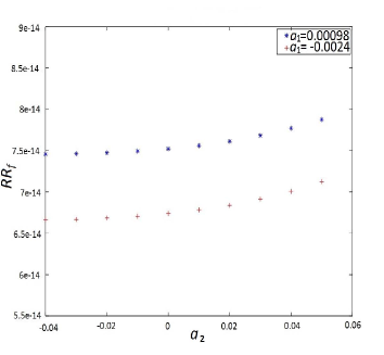
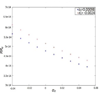
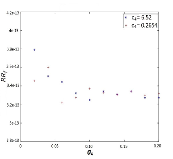
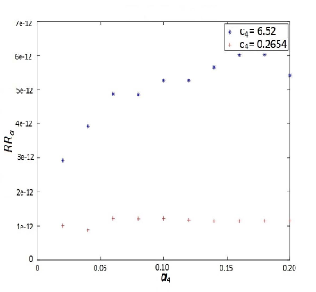
In the following figures we plot the relative residuals of and for the updated system for different parametric values of as mentioned in Corollary 4.1 for the case when . We plot by choosing and in Figure 1.
Example 5.2.
We consider this example from [43]. Consider the even quadratic matrix polynomial with
Let and . Then it is easy to verify that are eigenvalues of . Now it is necessary to determine the real perturbation matrices in such a manner that become the eigenvalues of the quadratic matrix polynomial whereas rest of the eigenpairs of are same as those unknown eigenpairs of . Then applying Remark 4.3 we have
and
such that is an invariant pair of . Using Remark 4.3 we choose the matrix
and obtain the real symmetric matrix
Therefore, we obtain the real matrices so that
and . Let denote the invariant pair corresponding to the fixed eigenpairs of Then the relative residuals of for the updated polynomial are given by
which ensures that the unknown eigenpairs of remains to be the eigenpairs of and are eigenvalues of the even matrix polynomial . Hence, eigenvalues are replaced successfully with maintaining no spillover on unmeasured eigenpairs of .
Moreover, choosing
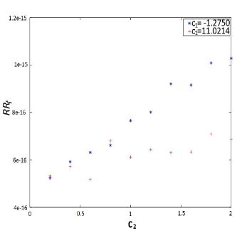
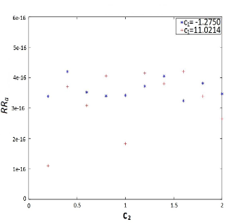
we plot the relative residuals of and for the updated matrix polynomial for various parametric values of as mentioned in Remark 4.3. In Figure 2, we plot choosing and .
Example 5.3.
In this example, we consider the matrices as randomly generated real symmetric positive definite matrices of order and is a randomly generated real skew-symmetric matrix of order . Let and . Suppose we want to replace the eigenvalues of by the desired scalars with maintaining no spillover effect on unmeasured eigenpairs of . Then applying Remark 4.3 we define the matrices accordingly and choosing the matrix
we obtain the real perturbation matrices with and , which ensures that are symmetric matrices while is a skew-symmetric matrix. It should be noted that is nearly zero, which implies that are eigenvalues of . Let denote the fixed invariant pair corresponding to the fixed eigenpairs of Then we have
Besides, is nearly zero, which guarantees that fixed eigenpairs of remain the eigenpairs of . Hence, it shows that a few eigenvalues of are replaced by the desired scalars with maintaining no spillover.
However, choosing
the relative residuals of and for the updated system has been plotted in the following figures for several parametric values of as given in Remark 4.3. In particular, we plot choosing and in Figure 3.
Conclusion. We consider the structure-preserving eigenvalue embedding problem (SEEP) for regular quadratic polynomials with symmetry structures. First we derive structure-preserving perturbations of a structured qudratic polynomial that reproduce a desired invariant pair and preserve an invariant pair (need not be known) of the unperturbed polynomial. Then we utilize these results for solving the SEEP for quadratic structured matrix polynomials which include symmetric, Hermitian, -odd and -even matrix polynomials. We show that the obtained solutions for SEEP correspond to existing results in the literature for certain structured matrix polynomials that arise in real-world applications. Finally, we illustrate the applicability of the obtained results through numerical examples.
References
- [1] B. Adhikari, B.N. Datta, T. Ganai, and M. Karow, Updating structured matrix pencils with no spillover effect on unmeasured spectral data and deflating pair, arXiv preprint arXiv:2003.03150, (2020), to appear in Linear Algebra and its Applications.
- [2] Z.-J. Bai, D. Chu, and D. Sun, A dual optimization approach to inverse quadratic eigenvalue problems with partial eigenstructure, SIAM J. Sci. Comput., 29 (2007), pp. 2531–2561.
- [3] Z.-J. Bai, B.N. Datta, and J. Wang, Robust and minimum norm partial quadratic eigenvalue assignment for vibrating systems: a new optimization approach, Mechanical Systems and Signal Processing 24 (2010), pp. 766-783.
- [4] J. Ball, and I. Gohberg, Interpolation of rational matrix functions, (Vol. 45). Birkhäuser, 2013.
- [5] M. Barkatou, P. Boito, and E.S. Ugalde, A contour integral approach to the computation of invariant pairs, Theoretical Computer Science, 681, (2017) pp. 3-26.
- [6] M. Baruch, Optimization procedure to correct stiffness and flexibility matrices using vibration tests, AIAA journal, 16 (1978), pp. 1208-1210.
- [7] A. Berman, and E.J. Nagy, Improvement of a large analytical model using test data, AIAA journal, 21.8 (1983), pp. 1168-1173.
- [8] R.V. Beeumen, K. Meerbergen, and W. Michiels, Computing a partial Schur factorization of nonlinear eigenvalue problems using the infinite Arnoldi method, SIAM Journal on Matrix Analysis and Applications, 36.2, (2015) pp. 820-838.
- [9] T. Betcke, and D. Kressner, Perturbation, extraction and refinement of invariant pairs for matrix polynomials, Linear Algebra Appl., 435.3 (2011), pp. 514-536.
- [10] W.J. Beyn, and V. Thümmler, Continuation of invariant subspaces for parameterized quadratic eigenvalue problems, SIAM Journal on Matrix Analysis and Applications, 31.3 (2010), pp. 1361-1381.
- [11] S. Brahma, and B.N. Datta, An optimization approach for minimum norm and robust partial quadratic eigenvalue assignment problems for vibrating structures, Journal of Sound and Vibration, 324 (2009) pp. 471-489.
- [12] J.B. Carvalho, B.N. Datta, W.W. Lin, and C.S. Wang, Symmetry preserving eigenvalue embedding in finite-element model updating of vibrating structures, Journal of Sound and Vibration, 290.3(2006), pp. 839-864.
- [13] J.B. Carvalho, B.N. Datta, A. Gupta, and M. Lagadapati, A direct method for model updating with incomplete measured data and without spurious modes, Mechanical Systems and Signal Processing, 21(7) (2007), pp. 2715-2731.
- [14] M.T. Chu, B.N. Datta, W.W. Lin, and S. Xu, Spillover phenomenon in quadratic model updating, AIAA journal, 46.2(2008), pp. 420-428.
- [15] D. Chu, M.T. Chu, and W.W. Lin, Quadratic model updating with symmetry, positive definiteness, and no spill-over, SIAM Journal on Matrix Analysis and Applications, 31 (2009), pp. 546-564.
- [16] M.T. Chu, W.W. Lin, and S.F. Xu, Updating quadratic models with no spillover effect on unmeasured spectral data, Inverse Problems, 23(1), (2007) pp. 243.
- [17] B.N. Datta, Finite-element model updating, eigenstructure assignment and eigenvalue embedding techniques for vibrating systems, Mechanical Systems and Signal Processing 16.1 (2002), pp. 83-96.
- [18] B.N. Datta, and D.R. Sarkissian, Feedback control in distributed parameter systems: a solution of the partial eigenvalue assignment problem, Mechanical Systems and Signal Processing 16 (1) (2001), pp. 3-17.
- [19] B.N. Datta, and D.R. Sarkissian, Theory and computations of some inverse eigenvalue problems for the quadratic pencil, Contemporary Mathematics, 280(2001), pp. 221-240.
- [20] B.N. Datta, S. Deng, V.O. Sokolov, and D.R. Sarkissian, An optimization technique for damped model updating with measured data satisfying quadratic orthogonality constraint, Mechanical Systems and Signal Processing, 23(6), (2009), pp. 1759-1772.
- [21] B.N. Datta, Numerical Linear Algebra and Applications, Vol. 116. Siam, 2010.
- [22] C. Effenberger, Robust successive computation of eigenpairs for nonlinear eigenvalue problems, SIAM Journal on Matrix Analysis and Applications, 34.3, (2013) pp. 1231-1256.
- [23] C. Effenberger, and D. Kressner, Chebyshev interpolation for nonlinear eigenvalue problems, BIT Numerical Mathematics, 52.4, (2012) pp. 933-951.
- [24] S. Elhay, Some inverse eigenvalue and pole placement problems for linear and quadratic pencils, Numerical Linear Algebra in Signals, Systems and Control, Springer, Dordrecht, 2011, pp. 217-249.
- [25] M. Friswell, and J.E. Mottershead, Finite element model updating in structural dynamics, Vol. 38, Springer Science and Business Media, 2013.
- [26] T. Ganai, and B. Adhikari, Preserving spectral properties of structured matrices under structured perturbations, arXiv preprint arXiv:2006.09434.
- [27] I. Gohberg, P. Lancaster, and L. Rodman, Indefinite Linear Algebra and Applications, Birkhäuser, (2005).
- [28] I. Gohberg, P. Lancaster, and L. Rodman, Matrix polynomials, Birkhäuser, (2005).
- [29] J.Z. Hearon, Nonsingular solutions of , Linear Algebra Appl., 16(1), (1977) pp. 57-63.
- [30] N.J. Higham, and H.M. Kim, Numerical analysis of a quadratic matrix equation, IMA Journal of Numerical Analysis 20.4 (2000), pp. 499-519.
- [31] B. Jaishi, and W.X. Ren, Damage detection by finite element model updating using modal flexibility residual, Journal of Sound and Vibration 290 (2006), pp. 369-387.
- [32] H.M. Kim, and T.J. Bartkowicz, Damage detection and health monitoring of large space structures, Journal of Sound and Vibration 27(6) (1993), pp. 12-17.
- [33] D. Kressner, A block Newton method for nonlinear eigenvalue problems, Numerische Mathematik, 114.2 (2009), pp. 355-372.
- [34] D. Kressner, and J.E. Roman, Memory‐efficient Arnoldi algorithms for linearizations of matrix polynomials in Chebyshev basis, Numerical Linear Algebra with Applications, 21.4, (2014) pp. 569-588.
- [35] Y.C. Kuo, W.W. Lin, and S. Xu, New methods for finite element model updating problems, AIAA journal, 44.6 (2006) pp. 1310-1316.
- [36] Y.C. Kuo, and B.N. Datta, Quadratic model updating with no spill-over and incomplete measured data: Existence and computation of solution, Linear Algebra Appl., 436.7(2012), pp. 2480-2493.
- [37] P. Lancaster, Model-updating for symmetric quadratic eigenvalue problems, (2006).
- [38] P. Lancaster, Model-updating for self-adjoint quadratic eigenvalue problems, Linear Algebra Appl., 428.11(2008), pp. 2778-2790.
- [39] J. Li, and X. Hu, A CG-Type Method for Inverse Quadratic Eigenvalue Problems in Model Updating of Structural Dynamics, Advances in Applied Mathematics and Mechanics, 3.1 (2011), pp. 65-86.
- [40] D.S. Mackey, N. Mackey, C. Mehl, and V. Mehrmann, Vector spaces of linearizations for matrix polynomials, SIAM Journal on Matrix Analysis and Applications, 28(4) (2006) pp. 971-1004.
- [41] D.S. Mackey, N. Mackey, C. Mehl, and V. Mehrmann, Structured polynomial eigenvalue problems: Good vibrations from good linearizations, SIAM Journal on Matrix Analysis and Applications, 28(4) (2006) pp. 1029-1051.
- [42] D.S. Mackey, N. Mackey, C. Mehl, and V. Mehrmann, Möbius transformations of matrix polynomials, Linear Algebra Appl., 470, (2015) pp. 120-184.
- [43] X. Mao, and H. Dai, Structure preserving eigenvalue embedding for undamped gyroscopic systems, Applied Mathematical Modelling 38.17-18 (2014), pp. 4333-4344.
- [44] X. Mao, and H. Dai, A quadratic inverse eigenvalue problem in damped structural model updating, Applied Mathematical Modelling 40.13-14 (2016), pp. 6412-6423.
- [45] J.E. Mottershead, and M.I. Friswell, Model updating in structural dynamics: a survey, Journal of Sound and Vibration 167.2 (1993), pp. 347-375.
- [46] J. Qian, Y. Cai, D. Chu, and R.C. Tan, Eigenvalue Embedding of Undamped Vibroacoustic Systems with No-spillover, SIAM Journal on Matrix Analysis and Applications, 38.4 (2017) pp. 1190-1209.
- [47] J.G. Sun, Backward perturbation analysis of certain characteristic subspaces, Numerische Mathematik 65.1 (1993) pp. 357-382.
- [48] D.B. Szyld, and F. Xue, Several properties of invariant pairs of nonlinear algebraic eigenvalue problems, IMA Journal of Numerical Analysis, 34.3, (2014) pp. 921-954.
- [49] F. Tisseur, and K. Meerbergen, The quadratic eigenvalue problem, SIAM review, 43(2001), pp. 235-286.
- [50] E.S. Ugalde, Computation of invariant pairs and matrix solvents, Doctoral dissertation, Université de Limoges, 2015.
- [51] D.C. Zimmerman, and M. Windengren, Correcting finite element models using a symmetric eigenstructure assignment technique, AIAA journal, 28 (1990) pp. 1670-1676.