Electric field reconstruction with three polarizations for the radio detection of ultra-high energy particles
Abstract
The amplitude, polarization, frequency spectrum and energy fluence carried by the electric field at a given measurement position are the key parameters for retrieving information from radio signals generated by extensive air showers. Accurate reconstruction of the electric field from the signals recorded by the antennas is therefore essential for the radio detection technique. Conventional reconstruction methods primarily focus on electric field reconstruction for antennas with two horizontal polarizations. In this paper, we introduce an analytical least-squares () reconstruction method that operates with both two and three polarizations, providing the reconstructed electric field at each antenna. This solution has been verified for simple and realistic antenna responses, with a particular focus on inclined air showers. Our method achieves an accuracy better than 4% in determining the Hilbert peak amplitude of the electric field and better than 6% accuracy on the estimation of the energy fluence, with minimal bias. Additionally, this was found to be reliable for almost any arrival directions, and the direction dependence has been investigated. This work also demonstrates that incorporating vertically polarized antennas enhances the precision of reconstruction, leading to a more accurate and reliable electric field estimation for inclined air showers. Consequently, the method enhances our ability to extract information about cosmic rays from the detected signals in current and future experiments.
1 Introduction
Cosmic rays with energies ranging from approximately 100 PeV to a few EeV mark a crucial transition in the energy spectrum, connecting Galactic and extragalactic origins. The “knee” at around 4 PeV likely reflects the rigidity-dependent cutoff of Galactic accelerators, while the “ankle” near 1 EeV signifies the increasing dominance of extragalactic sources. When the energy exceeds 1 EeV, it is called Ultra-high-energy cosmic rays (UHECRs). These particles possess energies beyond what laboratory accelerators can achieve, offering a unique opportunity to explore fundamental physics. Understanding cosmic ray composition and spectrum in this range provides insights into the mechanisms behind their acceleration and the interplay between Galactic and extragalactic magnetic fields [1, 2, 3, 4, 5].
The flux of high energy cosmic rays generally follows a steeply falling power law [6], resulting in an exceedingly low flux at high energies. Therefore, a large effective area is needed for a ground-based detector to collect adequate statistics of high energy cosmic rays within a reasonable time frame. Consequently, the primary detection method involves measuring extensive air showers (EAS) generated by their interactions with Earth’s atmosphere. One effective approach for detecting EAS is through the measurement of the radio signals they produce [7, 8].
Inclined air showers, a specific subset of EAS, with elevation angles up to 25∘, are excellent targets for studying UHE particles. They are typically triggered by UHECR at high altitudes, but can also be induced by UHE neutrinos interacting near the Earth’s surface, resulting in the shower maximum occurring close to the observer.
Due to atmospheric absorption of the particle cascade, particle detection techniques (PD) mostly measure the muon content of inclined air showers. Radio detection (RD), in contrast, provides direct access to the electromagnetic component and can thus complement particle detectors, offering additional advantages such as lower costs, full duty cycle, and high precision in reconstructing energy, Xmax, and arrival direction. The combination of RD and PD is particularly beneficial for enhancing sensitivity to mass composition [9, 10, 11, 12].
The radio emission from EAS is induced by the geomagnetic and Askaryan effects. The geomagnetic effect arises from the separation of electrons and positrons in the Earth’s geomagnetic field due to the Lorentz force in combination with their deceleration due to interactions with the atmospheric matter [13]. The separation generates a time-varying transverse current, leading to radio emission contributing the majority of the radiation energy. Recent simulations have shown that under high magnetic fields and low atmospheric density, the charged particles can be deflected over longer paths, causing the charged particles to gyrate and produce synchrotron-like emission as well as their emission losing coherence [14, 15]. The Askaryan effect also [16] contributes to the radiated energy, normally with less than 10% depending on the atmospheric density. This effect occurs whenever high-energy charged particles traverse a dense medium, causing additional electrons from the medium to be swept into the shower front through Compton scattering or ionization while the positive ions stay behind. This process creates a time-varying net charge excess at the shower front, resulting in radio emission.
A key feature of the radio emission is a Cherenkov ring in the footprint [17]. This ring forms due to the non-unity refractive index of the atmosphere, which varies with altitude. This creates a region of maximum coherence and leads to constructive interference in the observed signal on the ground. The energy fluence distribution on the ring is asymmetric, arising from the distinct orientations of the electric field vectors associated with the two primary emission mechanisms. The electric field resulting from the transverse current effect aligns with the direction of the Lorentz force, while the electric field from the Askaryan effect exhibits a radial symmetry pointing towards the shower axis. This results in different polarizations of the electric field with respect to the shower core.
Simulation and experimental investigations have benefited from each other to enhance our understanding of cosmic ray radio emission. Simulation tools such as CoREAS [18] and ZHAireS [19] are widely used for simulating radio emissions, offering a means to study the patterns of these emissions. Experimental efforts, exemplified by pioneering projects like LOPES [20] and CODALEMA [21], have demonstrated the feasibility of radio detection of EAS triggered by cosmic rays. Following the successful validation of this detection technique, numerous other radio experiments have been initiated; for a review we refer the reader to references [7, 8]. Recent projects have further proposed the use of pure radio detection methods, optimized for various air shower geometries, including inclined and upward-going air showers, as well as in-ice air showers [7, 8, 22, 23, 24]. These developments aim to establish self-triggering detection techniques using radio methods.
These radio-emission simulations and experiments paved the way for sophisticated reconstruction techniques. Sub-degree precision in direction reconstruction has been achieved by analyzing the peak time of each radio signal [9, 25, 26]. For vertical air showers, an ultimate energy resolution of 3% has been achieved in SKA [27, 28] due to its large antenna density and increased bandwidth. For inclined showers, a resolution well below 10% is expected from realistic end-to-end simulation studies on the basis of an analytical description of the radio-emission footprint and parameterization of the signal [29]. Furthermore, shower-to-shower fluctuations in the footprint for a fixed incident direction and energy have been utilized for reconstruction of shower maximum Xmax, achieving resolutions better than 15 g/cm2 at the highest energies in AERA [30] and expecting resolutions better than 8 g/cm2 in SKA with established techniques [27, 28, 31, 32, 33, 34].
The reconstruction of shower properties relies on accurate information about the electric field at the positions of radio detector units. However, radio antennas measure voltage signals, making it a crucial first step in all analyses to reconstruct the electric field from these voltage signals. The initial technique for reconstructing the electric field from voltage traces, involving the inversion of a 2×2 response matrix, was developed by AERA [35]. As shown in Ref [36], a minimization of the squared error of voltage in the Hilbert envelope helps to obtain a standard solution, which can help to reconstruct the electric field by taking the response of all the antenna channels into consideration. However, this method works reliably only with two polarizations for high signal-to-noise-ratios (SNR) events, and noise is ignored. Additionally, a forward folding technique based on the frequency slope employs the least-squares () method to give better results than this standard method even for events with SNR ¡ 10, with all the antenna channels being considered. A more recent and innovative technique employs information field theory to reconstruct signals with low SNR with high precision [38, 39]. These methods, however, have been applied primarily to antennas with only two horizontal polarizations, leading to incomplete sampling of the three-dimensional electric field.
Inclined air showers, in particular, exhibit higher signal strength in the vertical component of electric fields than vertical air showers, which highlights the importance of accurately capturing all polarization components of the signal. In this context, we introduce a new approach based on least square estimation for reconstructing the electric field, which incorporates not only the two horizontal polarizations but also the additional vertical polarization, allowing a more complete and precise reconstruction of the three-dimensional electric field.
This article is organized as follows: section 2 covers the simulations of radio emission, antenna response, and background noise used for reconstruction in our analysis. In section 3, we explain our reconstruction method, followed by an assessment of its performance in section 4. Finally, we provide a discussion and conclusions in section 5.
2 Simulations
Our work is based on detailed simulations of EAS and their radio emission. We first created a librariy of air shower events with their associated electric fields. Next, we incorporated specific antenna models to convert the electric field into voltage signals. Finally, we included a galactic noise model to account for environmental interference. By combining these elements, we generated simulated voltage data that closely matches experimental results, providing a robust foundation for reconstructing the electric field.
2.1 Simulation of cosmic ray radio signals
We used the ZHAireS simulation package [19] to simulate the radio emissions induced by EAS. We created a Monte Carlo (MC) dataset covering zenith angles from 63.0∘ to 87.1∘ in equidistant steps of , focusing specifically on inclined EAS. The azimuth angle spans from 0 to 180∘, with increments of 45∘. The primary particle energy ranges from 0.126 EeV to 3.98 EeV in logarithmic steps of 0.1. The simulation site is located in Dunhuang, a radio-quiet area in China. The geomagnetic field at this site has a strength of 56T and an inclination angle of 61 ∘. For the atmosphere, we use the extended Linsley standard atmosphere, in which an exponential index of refraction model was used, with scale height of 8.2km and sea level refraction index of 1.000325. Our simulation set is evenly divided between proton and iron primaries. A total of 4160 EAS events were generated for this analysis.
We employed a star-shaped configuration on the ground comprising 160 antennas in the simulation, organized into 8 arms with 20 antennas each. The ring spacing was adjusted to align with the Cherenkov angle, ensuring that the peak amplitude was located centrally within the entire simulated footprint. This adjustment aims to ensure robust footprint coverage, even under aggressive trigger conditions.
The components of the simulated electric field correspond to three polarization directions: (South-North), (East-West), and (Down-Up). We selected a time bin of 0.5 ns within a 1000 ns time window, which provides a frequency resolution of 1 MHz after performing a Fourier transformation.
2.2 Antenna responses
When using only horizontally aligned antennas, a significant portion of events coming close to the horizon cannot be detected, as a significant part of the signal will be vertically polarized. To achieve full sky coverage, it is essential to include an additional antenna arm oriented vertically [40], or have two antennas that are partly sensitive to the vertical component as the case for the SALLAs in Auger-RD [41].
This study tests two types of antennas to reconstruct the electric field with three polarizations: a simple 3-arm dipole antenna, which has symmetrical oscillators for the horizontal arms, and a more complex 3D bow-tie-shaped HORIZON antenna [22, 42]. The dipole antenna serves as a baseline for developing the reconstruction method, while the HORIZON antenna is used for verification and performance evaluation for a realistic setup. Antenna responses were simulated using Ansys HFSS [43], with all simulations incorporating ground effects to ensure accurate representation of real-world conditions. The antenna response patterns are shown, for a representative frequency, in Appendix A.
2.2.1 Dipole antenna
The first type of antenna we use in our study is a dipole antenna featuring three polarizations. Each of the three arms consist of two oscillators, each measuring 1.3 meters, resulting in a total length of 2.6 meters per arm. The entire antenna is positioned 3 meters above the ground and operates within a frequency range of 30 to 80 MHz, making it suitable for radio detection experiments. The horizontal arms are aligned along the South-North (SN) and East-West (EW) directions, with the vertical arm representing the Z polarization. In this context, the geomagnetic north is defined as the x-axis, and the east is the y-axis. This design was initially implemented in the LOPES-3D experiment [44, 40].
Figure 1 illustrates the antenna’s response in the three directions, with polarizations represented in spherical coordinates . Two examples with varying zenith and azimuth angles are provided. In both cases, there is a single resonance within the 30-80 MHz range, resulting in a relatively smooth variation across the frequency band, with only minor irregularities near the upper end of the range.

2.2.2 HORIZON antenna
The HORIZON antenna is designed with a more complex structure to enhance its capability of detecting inclined EAS while maintaining sensitivity to less inclined showers. It consists of a symmetric steel radiator with three mutually perpendicular antenna arms. This bow-tie-shaped antenna features three polarizations, each of the 3 arms is composed of a symmetric butterfly-shaped steel radiator. It contains a dipole in each of the X, Y-arms, and a monopole in the Z-arm.
To provide the fairest possible comparison with the dipole case, the entire antenna is positioned 3 meters above the ground. This is 0.2 meters lower than the original design specified in [45].
The antenna arms are aligned in the same directions as described for the dipole antenna. The antenna operates within the 50-200 MHz frequency range and is equipped with a purposely designed matching network. The design prioritizes phase center consistency, although this compromises its omnidirectionality. This antenna type was inspired by the ”butterfly antenna” used in the CODALEMA project [46], and it has been further refined and deployed in the GRAND experiment [22, 42].
Increasing the bandwidth of the antenna to four octaves introduces frequency-dependent lobes in the antenna beam. Despite this complexity, as the radio signal from EAS covers a broad frequency range and arrives from various directions, this antenna achieves an efficient overall interception of the incoming electric field energy. Figure 2 illustrates the HORIZON antenna’s response following the same conventions as in Fig. 1.Unlike the dipole antenna, this antenna exhibits multiple resonant frequencies. For instance, at a zenith angle of 67.8∘ and an azimuth angle of 45∘ in the East-West polarization, there are two resonant frequencies in the -component, while the -component shows nearly zero gain around 60 MHz and 180 MHz. More resonances are observed in the vertical polarization. This complexity poses a challenge for electric field reconstruction, and will be discussed in section 3.3.

2.3 Electric field to voltage
The open-circuit voltage is a convolution of equivalent length (antenna response) as shown in Figure 1 and 2, and electric field:
| (2.1) |
where represents the measured voltage, is the vector equivalent length (VEL), is the electric field, and denotes the convolution operation. For simplification purposes, calculations are often performed in the frequency domain through Fourier transformation, yielding the expression [47]:
| (2.2) |
where , and are voltage, VEL, and electric field respectively in the frequency domain after Fourier transformation.
2.4 Background noise
Reconstructing radio signals is challenging due to the complexity of various background noise sources present at the site. Most of the radio emission power is concentrated in the frequency range below 200 MHz. To mitigate the impact of human activities such as radio telecommunications and navigation, radio detection experiment sites are chosen to be located far from urban areas. While thunderstorms, solar flares, subterranean pre-seismic movements, and other intense radio activities can generate complicated background noise, they are only active at certain times and are not included in this work. In this scenario, the galactic background is considered to be the predominant noise source in the specified frequency band [48]. This type of noise, which marked the birth of radio astronomy, was first identified by Karl Jansky and originates from the diffuse synchrotron radiation within the Galaxy [49].
To model the background noise spectrum in the range of [30, 200] MHz, the LFmap model [50] is utilized. This model includes various components such as the Cosmic Microwave Background (CMB), isotropic elements, Galactic sources, and extragalactic sources. The sky temperature follows a power law in this context:
| (2.3) |
The brightness can be derived from the sky temperature using the Rayleigh-Jeans approximation: , where is the Boltzmann constant, and is the speed of light. The power of sky noise is then expressed as:
| (2.4) |
where represents the local sidereal time (LST), is effective receiving area of the antenna (obtained from the antenna gain), and the antenna efficiency . The effective area is given by , where is the antenna gain, G=1 for a lossless resonant antenna of impedance matching the load. The left panel of Figure 3 shows this background power spectrum in East-West polarization.
Here, we do not consider any specific antenna design but assume a typical antenna impedance of , corresponding to an ideal impedance match. In practice, antenna impedance varies with frequency and may deviate from this idealized assumption. However, this simplification provides a consistent noise level, ensuring a reliable baseline for comparison despite potential discrepancies with real-world scenarios. With impedance matching, half of the power is transferred to the receiver. Consequently, the voltage received from the background can be expressed as:
| (2.5) |
The right panel of Figure 3 shows the RMS of the Galactic noise in the time domain as a function of the LST in East-West polarization.

Since the voltage spectrum of the noise is known and can be approximated as white noise, we generated a uniformly distributed phase that was added to this spectrum. By performing an inverse Fast Fourier Transform (iFFT), we obtained the noise trace in the time domain, which was then added to the signal’s voltage trace.
Thermal noise in the electronics of the Radio Frequency (RF) chain also contributes to the overall noise. However, this noise is added independently at each polarization after the open circuit voltage. Since our focus is on the reconstruction from open circuit voltage to electric field, electronic noise is beyond the scope of this article.
3 Electric field reconstruction
As mentioned in Section 2.1, the electric field in the simulations is provided in Cartesian coordinates. Since electromagnetic waves in the air are transverse waves, the component along the propagation direction, , is negligible. Consequently, we can reduce one degree of freedom. Expressing the convolution more conveniently using spherical coordinates:
| (3.1) |
where is open circuit voltage, subscripts 1,2,3 in represent three polarizations of antenna, and , and are the spherical coordinate components of each polarization. represents the noise added in each polarization and we choose the sky map corresponding to LST=18h, which represents a relatively high noise level at each polarization.
The grey lines in Figure 1 and 2, show that the component is indeed a small quantity. Hence the 3 by 3 response matrix can be reduced to 3 by 2.
| (3.2) |
In this paper, we use two approaches for reconstructing the electric field. The first is a matrix inversion method,commonly employed in most radio experiments, which involves inverting the response matrix using either two or three polarizations (section 3.1), while the second method is a least square method using three polarizations (section 3.3). The latter is the approach introduced for the first time in this study.
3.1 Matrix inversion method
When the SNR is large enough in all the traces in the full frequency band, and given the signal’s arrival direction, two orthogonal horizontal polarizations are sufficient to give a good reconstruction of the electric field. This has been implemented in most radio experiments [47, 51]. The electric field can be reconstructed by inverting Equation 3.2 using any two voltage polarizations, expressed as . In this approach, noise is considered to be small enough to assume that is equal to .
| (3.3) |
In the absence of noise, this method yields an exact solution for the electric field. With the inclusion of an additional polarization, the electric field can be reconstructed in three different combinations, as demonstrated first in LOPES 3D. Since different polarizations are sensitive to varying incident angles, LOPES 3D employed a strategy of weighting the reconstructed electric field based on the zenith angle [44].


3.2 Two polarizations vs. three polarizations with matrix inversion method
Although the component is small, it is non-zero, making it possible to solve the inverse matrix in Equation 3.1. This allows us to include the third polarization, which is expected to improve the signal by providing additional information.
| (3.4) |
We compare this approach with the conventional 2 polarizations method using a simple dipole model in the 30-80 MHz frequency band. The example we present shows voltage traces with an SNR of approximately 6 in each polarization. Here, the SNR is defined as /RMSnoise, where signal S is the maximum value of the Hilbert envelope of the voltage, and the root mean square (RMS) of noise is associated with the standard deviation in a 250 ns noise window located 500 ns after the signal peak. Figure 4 illustrates the signals in the three polarizations.
The reconstruction results for this example are shown in Figure 5, and Table 1 provides a quantitative comparison in the time domain through normalized cross-correlation values between the reconstructed and simulated (Monte Carlo true) traces. We take the normalized cross-correlation from [52] which is used to check the agreement of interpolated pulse shape and is defined as:
| (3.5) |
where represents the simulated electric field trace, represents the reconstructed trace, and is the trace length. And is the time mismatching between these two traces, in our case .


| Reconstruction | Normalized cross-correlation | |
|---|---|---|
| -component | -component | |
| 2 polarizations (matrix inversion) | -0.13 | 0.93 |
| 3 polarizations (matrix inversion) | 0.40 | 0.80 |
For the -component of the electric field, which carries a relatively stronger signal, both the two-polarization and three-polarization reconstruction methods produce similar results. As shown in the upper right panel of Figure 5, the simulated and reconstructed traces overlap closely. In the frequency domain (lower right panel), while the three-polarization method introduces spikes, it still achieves a normalized cross-correlation of around 0.80, slightly underperforming the two-polarization method. For the -component (left panel), which has a weaker signal, the differences between the methods become more evident. The three-polarization method shows fluctuations at specific frequencies, whereas the two-polarization method exhibits larger deviations toward the end of the spectrum. This is reflected in the negative cross-correlation value for the two-polarization approach, indicating greater errors and a noticeable peak time shift observed in the time-domain trace.
The spikes in the spectrum for the three-polarization reconstruction, as shown in the bottom panel of Figure 5, are due to the very small values of the -component, which cause divergence at certain frequencies.
3.3 Analytical solution with least Chi-Square estimation for each antenna
To eliminate the divergence at certain frequencies in the three-polarization reconstruction, we employ a robust least squares estimation method. This approach enables a minimization process without requiring any prior assumptions about the electric field spectrum, thereby enhancing the reliability of the reconstruction. By accounting for noise and minimizing the influence of small -components, this method ensures more stable and accurate results across the frequency spectrum.
We build a based on antenna response, noise spectrum and measured voltage:
| (3.6) | ||||
where is the voltage in the 3 polarizations, and is the antenna response shown in Equation 3.2. Since the antenna response depends on the direction of the EAS, we use the true direction from simulations in this study. The choice is based on the observation that the antenna response does not exhibit abrupt changes with direction, and the directional resolution provided by the plane wave reconstruction suffices for this case. A brief discussion on the impact of directional smearing is provided in section 4.2.3. The electric field is represented as . We assume that the error in this measurement is introduced by background noise. Therefore, the covariance matrix is given by the square spectrum of it.
Taking the derivative to minimize :
| (3.7) |
We get an analytical solution of electric field [53]:
| (3.8) |
The global minimum does not assure a minimum on each antenna arm, but by doing the minimization processes on three polarizations simultaneously, a better overall accuracy is obtained. Additionally, as with all kinds of minimization procedures, we must make sure that the scanning algorithm of the parameter space and the sample size are adequate to drop out the uncertainty in the reconstruction. In this work, the analytical least-squares () method directly provides the reconstructed electric field on each antenna arm using just the measured voltage, antenna response and background noise spectrum, which is more straightforward than the other methods.
In experiments, degradation of the antenna array can occur over time, some antennas may be broken or damaged, consequently their responses may also change due to some reasons. In this case, this analytical least-squares () method is still reliable, since the minimization on each antenna is not influenced by the unreliable antennas.
3.4 Matrix inversion method vs. analytical least Chi-Square solution
In Figure 6, we present a comparison between our analytical least-squares () method and the matrix inversion approach for reconstructing the electric field for the dipole antenna. The time-domain traces exhibit smaller fluctuations in the non-signal time window, and the spectrum is free of spikes, both of which highlight the improved reconstruction achieved using the analytical least-squares () method.

To evaluate the performance of the analytical least-squares () method, we again employ Equation 3.5 for comparison with the matrix inversion method. We found the analytical least-squares () method effectively minimizes noise-induced distortions and ensures more stable results. The normalized cross-correlation values listed in Table 2 show that the analytical least-squares () solution yields values better than those of the matrix inversion method for both components, confirming better performance in reconstructing the electric field.
| Reconstruction | normalized cross-correlation | |
|---|---|---|
| -component | -component | |
| 3 polarizations (matrix inversion) | 0.40 | 0.80 |
| 3 polarizations (lsq) | 0.77 | 0.95 |
3.5 Application to the HORIZON antenna


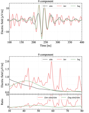
To confirm that our method is not highly dependent on the specific antenna response and frequency bandwidth, we applied it to the HORIZON antenna (see Sec. 2.2.2), which operates over a broader frequency band. Using the same simulation parameters as those for the dipole antenna example, we examined the differences in reconstruction under the same near threshold conditions. This particular signal has larger horizontal component than vertical ones, as shown in Figure 7. This comparison highlights the robustness of our method across different antenna designs and signal conditions.


The reconstruction results are shown in Figure 8. The -component (right panel) is well reconstructed with the analytical least-squares () method, while the -component (left panel), which has weaker signals, shows significant inaccuracies with the matrix inversion method (shown in coral). The bottom panel of Figure 8 compares the spectra, providing a detailed assessment of reconstruction quality.
| Reconstruction | normalized cross-correlation | |
|---|---|---|
| -component | -component | |
| 3 polarizations (inv) | -0.34 | 0.96 |
| 3 polarizations (lsq) | 0.79 | 0.97 |
It is important to note that with an azimuth angle of , the response is symmetric for horizontal polarizations, and the vertical component’s response is only sensitive to the -component. For -component, there is a bump that occurs around 120MHz due to the low antenna gain at this frequency,as illustrated by the solid line for the horizontal component in Figure 2. The time-domain trace is not significantly affected, as shown by the normalized cross-correlation value being close to 1 . For the -component, the matrix inversion method performs much worse than the least-squares approach, a large deviation appears around 60MHz, mainly due to the low antenna gain in the -component at this frequency, where the gain is primarily derived from the vertical polarization. The fluctuations at the higher end of the spectrum result from both signal weakening and reduced antenna response at those frequencies. Although both methods exhibit deviations, the analytical least-squares () method provides better accuracy (see normalized cross-correlation value in Table 3).
4 Statistical performance of the analytical least Chi-Square method
We now estimate the resolution of the analytical least-squares () method using a large number of traces from the simulations described in section 2.1 and the two antenna models introduced in section 2.2.
4.1 Event selection
Before the statistical analysis, we must select the events that can be distinguished from the background noise. The selection criteria for identifying simulated signals are informed by the characteristics of the simulated voltage and the background noise. The following criteria are intended to ensure that the detected signals are genuine:
-
•
SNR 5 for any of the 3 polarizations.
-
•
ns ¡ ¡ + 200 ns : the time of the maximum amplitude of the trace, , must fall within ns of the time the signal is expected to be on the trace.
-
•
Only the innermost 16 antennas out of the 20 simulated antennas of each arm of the star-shape pattern are used. The simulation footprint covers twice the Cherenkov angle, and antennas beyond number 16 are excluded because they do not capture significant coherent signals.
-
•
5 : at least 5 antennas must meet the above criteria for the simulation event to be selected, which is a typical requirement for cosmic ray reconstruction.
For the dipole antenna, 2332 out of 4160 simulations pass these event selection criteria. In these selected events, 79% of the antennas were triggered according to the above conditions. For the HORIZON antenna, 2749 simulations passed the selection criteria, from which 71% of the antennas were triggered. This selection process does not introduce bias with respect to the initial parameters, such as zenith angle, azimuth angle, or energy.
4.2 Hilbert peak amplitude comparison
The Hilbert envelope offers a smooth, amplitude-tracking representation of the signal, making it especially useful for handling oscillatory or noisy data. We use the peak value of the Hilbert envelope of the reconstructed electric field for comparison between true and reconstructed traces. The relative error distribution is shown in Figure 9.

The distribution shows that the reconstruction method performs robustly for both antenna types, with the relative error distributions approximately centered, indicating reliable accuracy in reconstructing the electric field. However, differences in bias and error distribution are observed between the dipole and HORIZON antennas.
For the dipole antenna, the results exhibit a relative error of 0.03, with a mean and median bias of 0.05, which suggests a slight underestimation in the reconstruction using this method. The slight asymmetry in on either side further reflects this bias.
HORIZON antenna shows a smaller bias, with a mean and median of 0 indicating a closer alignment with the true signal. However, the HORIZON antenna also exhibits a slightly broader error distribution, with a standard deviation (std) of 0.04, particularly in the -component with std of 0.12. This broader spread is likely attributed to the antenna’s response, which prioritizes sensitivity to inclined air showers. The larger frequency bandwidth of the HORIZON antenna contributes to increased variability in the -polarization, thereby accumulating greater errors. Nonetheless, these results indicate that the analytical least-squares () method achieves robust reconstruction performance with the HORIZON antenna.
For both antennas, the -component, representing the horizontal polarization, is generally reconstructed with higher precision compared to the -component. As shown in Figure 1 and Figure 2, the -component benefits from stronger signals and better antenna gain in most of the frequency band. This trend is more pronounced for the HORIZON antenna, which shows higher variability in the -component in its broader frequency band.
In conclusion, the overall relative error of reconstruction remains small for both antenna types, despite minor variations in bias and difference in relative error. This consistency underscores the robustness of the analytical least-squares () method for electric field reconstruction in cosmic ray studies.
4.2.1 Two polarizations vs. three polarizations with the analytical least Chi-Square method
As discussed in section 3.2, the vertical polarization enhances reconstruction precision when the electric field is reconstructed with the matrix inversion method. This holds true for the analytical least-squares () method as well. We will use , the range containing 34% of events on either side of the most probable value of the relative error distribution, to compare the resolution of the results obtained using 2 and 3 polarizations independent of bias. Figure 10 shows the of the Hilbert peak as a function of SNR.
Adding the vertical polarization significantly improves the reconstruction accuracy across all the SNR range by a factor of 3 to 5, or even more at low SNR, underscoring the critical role of the vertical polarization in refining the reconstruction of the electric field.

4.2.2 Dependence on arrival direction

As the electric field is convolved with the antenna response, which depends on the arrival direction of the air shower, the resolution of our method is inherently influenced by directionality. Different types of antennas are sensitive to different incident angles, leading to natural, albeit small, variations in precision. This directional dependency is illustrated in Figure 11.
For both antennas, total of the relative error distribution of the Hilbert peak of the reconstructed electric field varies symmetrically with respect to the azimuth angle at /2, ranging from 0 to . It initially increases and then decreases, mirroring the symmetric nature of the antenna responses, both in the - and-polarizations, as shown in Figure 17 on appendix A. Specifically, in the -component, the effective length decreases from 0 to /2, while in the -component, it increases within the same range. The interplay between these two components results in the observed initial rise and subsequent decline in resolution.
However, the relationship between zenith angle and precision differs between the two antennas. For the dipole antenna, precision decreases as the zenith angle increases, which is primarily due to the reduced signal strength at larger zenith angles, even though the effective length of the dipole antenna shows only a small increase with increasing zenith angle (see left panel of Figure 17 in Appendix A). In contrast, for the HORIZON antenna, the precision does not follow a consistent trend with zenith angle, there is a small dip around 80° (see left panel of Figure 18 in Appendix B). This is because the antenna response (see right panel of Figure 17 in Appendix A), is non-monotonic across whole zenith range. Consequently, the complex variations in precision are influenced by both the irregular antenna response and the changes in signal strength.
As shown in Figure 11, we observe that for the dipole antenna, no event is selected at azimuth angle = 0 or and zenith angle . For this arrival direction, the polarization of the geomagnetic transverse current is parallel to , so the strongest signal comes from this direction, while the antenna gain is minimal at these azimuth angles for both antennas (see Figure 17 in Appendix A). This lack of selected events has not been found with the HORIZON antenna. Despite its larger standard deviation at azimuth angle in [45∘, 135∘] when zenith angle 85∘, the broader frequency band of the HORIZON antenna allows for more signal to be captured, which results in more selected events. In this aspect, the HORIZON antenna is specifically suitable for detecting inclined air showers, which is consistent with the discussion presented in section 2.2. However, as the complicated shape of the HORIZON antenna makes it’s equivalent length to decrease strongly in certain ranges of air shower incoming direction (see the right panels of Figure 17 and 17 in Appendix A), this will produce larger deviations if the incorrect incoming direction is used.
In conclusion, the analytical least-squares () method shows robust performance in reconstructing the electric field for inclined air showers across a wide range of arrival directions. For directions where the signal-to-noise ratio is sufficiently high, the method achieves precise and reliable reconstruction, validating its effectiveness for this application.
4.2.3 Deviation of arrival direction
In offline analysis, sub-degree precision in direction reconstruction is traditionally achieved by analyzing the spatial distribution of electric field arrival times on the ground [9, 25, 26]. However, an accurate reconstruction of the electric field depends on the antenna response, which in turn requires the arrival direction as input. Although further refinements could incorporate an iterative direction reconstruction, here we present a straightforward analysis to demonstrate that a small deviation in direction (on the order of one degree) has minimal impact on the electric field reconstruction, ensuring the desired precision remains intact.
We artificially smeared the shower direction, deviating it from the true direction, following a Gaussian distribution with a standard deviation of degree in both zenith and azimuth angles. This level of deviation is of the order of the Cherenkov angle in air, and larger than the angular resolution obtained from direction reconstruction methods using timing information and wavefront analysis[25].

Figure 12 displays the relative error distribution of the Hilbert peak of the reconstructed electric field for both the dipole and HORIZON antennas. While the distribution of the dipole antenna remains almost unaffected, the tail in the results of the HORIZON antenna shows a tendency to overestimate the Hilbert peak, indicating a decrease in resolution. We analyze this result for the HORIZON antenna further in Figure 13. The left panel depicts the relative error distribution of the HORIZON antenna, separately for events below and above a zenith angle of , highlighting that most deviations cluster at large zenith angles. The right panel examines how this changes with SNR and zenith angle deviations. For electric field reconstructions with larger error, no strong correlation with SNR is observed. However, the cases with a relative error greater than 1 primarily correspond to zenith angle deviations exceeding 1∘. However, relative errors exceeding 1 are primarily associated with zenith angle deviations greater than 1∘. This asymmetry arises because, at specific zenith angles, the antenna response falls between two side lobes, a feature inherent to its broad frequency bandwidth.

4.3 Energy fluence comparison
The electromagnetic component of an air shower carries the majority of the energy of the primary particle Eshower, and the electromagnetic energy Eem can be estimated directly from the radiation energy [54]. For each antenna, the radio signal pulse determines the energy deposition per unit area, called energy fluence. For an antenna array, the spatial integral over the energy fluence measures the radiation energy from the primary particle in the working frequency band of the antennas. Hence, we can reconstruct the primary energy from the reconstructed electric field.
The energy fluence is defined as the integral of the squared electric field within the signal time window, which represents the total deposited energy per area accumulated at the location of the antenna.
| (4.1) |
with as the reconstructed electric field, c the light speed in vacuum and the permittivity in vacuum.

For coherent emission, the radio pulse amplitude is proportional to the electromagnetic energy of the air shower, so E [54, 55, 38].
Radio emission starts from the starting point of the electromagnetic interaction, carrying information at each stage of air shower development until the end of it. The typical duration of radio emission is of order several nanoseconds. We selected a 100 ns time window symmetrically centered around the signal peak and a 100 ns window at the end of the trace to estimate the fluence of the noise. The background noise fluence is subtracted from the fluence calculated for the signal window to calculate the signal energy fluence. Figure 14 displays the relative error distribution in energy fluence, which exhibits a similar trend to the Hilbert peak distribution but with more pronounced discrepancies since the error in the energy fluence accumulates from the squared electric field error. This increased deviation is attributed to the fact that noise accumulates over time during the integration process and cannot be completely filtered out.
For the dipole antenna, the median underestimation persists at 3%, which is consistent with the bias observed in the Hilbert peak analysis. While the HORIZON antenna exhibits no bias in energy fluence. Notably, the -component exhibits worse performance in both antenna types due to the relatively weaker signal in this component.
In terms of overall precision, the standard deviation in energy fluence is approximately 6%, with the HORIZON antenna displaying a more asymmetric range of [-0.04, 0.01]. In contrast, the dipole antenna shows a 4% standard deviation in total energy fluence with a more symmetric distribution of [-0.04, 0.03]. Despite these differences, both antennas enable precise reconstruction, demonstrating the method’s effectiveness.

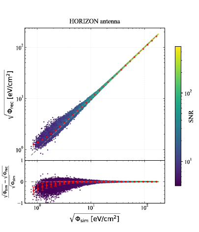
Figure 15 compares the reconstructed and simulated square root of energy fluence , which is proportional to Eem. For each event, the SNRs on the antennas vary depending on the distance and viewing angle to the shower maximum. Additionally, for each antenna, the sensitivity of the 3 arms also depend on the air shower direction, leading to SNR differences in each channel. We classify events by SNR, and we found our least-squares method yields accurate energy fluence estimates at high SNRs (10) for both types of antennas, while at lower SNRs, increased deviations are observed, which indicates bigger uncertainties in the reconstruction of shower energy Eshower.
5 Conclusions and outlook
The radio detection technique for EAS has been well-established, prompting current efforts to enhance detection capabilities across a broad frequency spectrum and for larger zenith-angle events. In particular, optimizing antennas for detecting ice and air showers induced by UHE neutrinos, a goal for the next generation of detectors, is of paramount importance. Adding a vertical polarization to antennas enhances their sensitivity to electric field signals, as it allows for capturing the full three-dimensional electric field. This improvement facilitates more accurate signal reconstruction, particularly for events with significant vertical components, and demonstrates the advantages of the three-polarization approach in radio analysis.
We have seen that the matrix inversion approach to reconstruct the electric field struggles when trying to reconstruct near-threshold signals (SNR around 5).
Without making any assumptions about the electric field spectrum, we have introduced an analytical least-squares () method to reconstruct the electric field on each antenna. This was developed with the dipole antenna and then tested with the HORIZON antenna which has a more complicated response. LFmap-generated galactic noisewas added to the signals before the reconstruction. For both antennas, our approach achieves a standard deviation less than 4% in the Hilbert peak value with bias variations specific to each antenna that could be corrected accordingly. We found that adding a vertical polarization significantly improves the reconstruction accuracy by approximately one order of magnitude. This highlights the importance that a three polarization antenna allows for the effective extraction of information even from weak signals with limited precision.
The accuracy of this method depends on the signal arrival direction, which is an input in the first step of the reconstruction. We have performed two tests to evaluate this dependence. First, we generated a two-dimensional plot in direction of the total relative error in the Hilbert peak of the reconstructed electric field, and a resolution better than 4% was found for both the dipole and HORIZON antennas. Second, we have shown the effect of directional reconstruction precision into the analysis. A deviation of 1∘ is set to estimate the influence of this effect. We have found that the dipole antenna does not show significant relative error in the Hilbert peak of the reconstructed electric field, while the HORIZON antenna presents bigger errors for air shower with zenith angle 85∘. These larger errors, often associated with zenith deviations exceeding 1∘, highlight the dependence of the accuracy that can be obtained with the reconstruction method on the shape of the antenna response. If the antenna response changes rapidly with incoming direction, then a good direction reconstructions becomes paramount. An iterative reconstruction procedure could be incorporated to refine the reconstruction of the incoming direction and then further improve the electric field reconstruction. In any case, this has no significant impact on the overall resolution, as the number of such cases is statistically small.
The uncertainty in the reconstructed electric field accumulates in the integration used to calculate the radiation energy and ultimately spreads to the uncertainty of the shower energy. The good performance of the analytical least-squares () method leads to a precise determination of the energy fluence for high SNR events. Both the dipole and HORIZON antenna show good but different statistical performances at low SNR due to the different characteristics of their antenna responses.
We have shown that this method is versatile for radio detection, provided that the local noise is thoroughly understood. The noise model in this work contains only the LFmap galactic noise. Usage of noise data measured by a real antenna array on an experimental radio sites would be helpful for conducting a realistic test.
In this work we have tested the frequency band in [30, 200] MHz, which is covered by several experiments. For experiments going beyond this range, further studies will be needed. The signal strength at high frequency decreases more rapidly when the antenna viewing angle deviates further from the Cherenkov ring, where the signal in lower frequency usually dominates. In the frequency band we are studying, we have not split it into sub-bands for a detailed description, which could be explored further.
The reconstruction method we presented in this work makes no assumptions on the signal spectrum slope, its polarization, energy contribution from the emission effects or other signal characteristics.
An iterative approach, in which the reconstructed shower direction is used again as input of the electric field reconstruction, can be used to repeat the direction reconstruction and improve the overall performance. This approach can be further enhanced by combining it with core position reconstruction, where the maximum amplitude of the Hilbert envelope of the signals can be used to iteratively refine the location of the shower core. By incorporating a more precise direction of the emission region and an accurate estimation of the distance to the antennas, the reconstruction process is expected to achieve a greater overall precision, leading to improved accuracy in determining the energy, composition, and arrival direction of the primary cosmic ray.
Acknowledgments
We would like to thank Kaikai Duan, Xiaoyuan Huang, Jiale Wang, Jean-Marc Colley and all the other GRAND members for the related discussions. This work is supported by the National Natural Science Foundation of China (Nos. 12273114), the Project for Young Scientists in Basic Research of Chinese Academy of Sciences (No. YSBR-061), and the Program for Innovative Talents and Entrepreneur in Jiangsu, and High-end Foreign Expert Introduction Program in China (No. G2023061006L). C.Z thanks Zhuo Li and Ruoyu Liu for their support and discussions during this work.
Appendix A Antenna response


Appendix B Direction dependence in specific angle

References
- [1] J. Blümer, R. Engel and J.R. Hörandel, Cosmic rays from the knee to the highest energies, Progress in Particle and Nuclear Physics 63 (2009) 293–338.
- [2] Pierre Auger collaboration, Measurement of the Energy Spectrum of Cosmic Rays above eV Using the Pierre Auger Observatory, Phys. Lett. B 685 (2010) 239 [1002.1975].
- [3] M. Ackermann et al., High-energy and ultra-high-energy neutrinos: A Snowmass white paper, JHEAp 36 (2022) 55 [2203.08096].
- [4] A. Coleman, J. Eser, E. Mayotte, F. Sarazin, F. Schröder, D. Soldin et al., Ultra high energy cosmic rays the intersection of the cosmic and energy frontiers, Astroparticle Physics 149 (2023) 102819.
- [5] B.T. Zhang, K. Murase, N. Ekanger, M. Bhattacharya and S. Horiuchi, Ultraheavy ultrahigh-energy cosmic rays, 2024.
- [6] P. Abreu, M. Aglietta, J.M. Albury, I. Allekotte, A. Almela, J. Alvarez-Muñiz et al., The energy spectrum of cosmic rays beyond the turn-down around ev as measured with the surface detector of the pierre auger observatory, The European Physical Journal C 81 (2021) .
- [7] T. Huege, Radio detection of cosmic ray air showers in the digital era, Physics Reports 620 (2016) 1–52.
- [8] F.G. Schröder, Radio detection of cosmic-ray air showers and high-energy neutrinos, Progress in Particle and Nuclear Physics 93 (2017) 1–68.
- [9] W. Apel, J. Arteaga-Velázquez, L. Bähren, K. Bekk, M. Bertaina, P. Biermann et al., The wavefront of the radio signal emitted by cosmic ray air showers, Journal of Cosmology and Astroparticle Physics 2014 (2014) 025–025.
- [10] P. Bezyazeekov, N. Budnev, D. Chernykh, O. Fedorov, O. Gress, A. Haungs et al., Reconstruction of cosmic ray air showers with tunka-rex data using template fitting of radio pulses, Physical Review D 97 (2018) .
- [11] T. Huege, The radio detector of the pierre auger observatory – status and expected performance, EPJ Web of Conferences 283 (2023) 06002.
- [12] F. Schröder, Design and expected performance of the icecube-gen2 surface array and its radio component, in Proceedings of 9th International Workshop on Acoustic and Radio EeV Neutrino Detection Activities — PoS(ARENA2022), ARENA2022, p. 058, Sissa Medialab, May, 2023, DOI.
- [13] F.D. Kahn and I. Lerche, Radiation from cosmic ray air showers, Proceedings of the Royal Society of London. Series A. Mathematical and Physical Sciences 289 (1966) 206.
- [14] C.W. James, Nature of radio-wave radiation from particle cascades, Phys. Rev. D 105 (2022) 023014 [2201.01298].
- [15] S. Chiche, C. Zhang, F. Schlüter, K. Kotera, T. Huege, K.D. de Vries et al., Loss of coherence and change in emission physics for radio emission from very inclined cosmic-ray air showers, Phys. Rev. Lett. 132 (2024) 231001.
- [16] G.A. Askaryan, Excess Negative Charge of the Electron-Photon Shower and Coherent Radiation Originating from It. Radio Recording of Showers under the Ground and on the Moon, Journal of the Physical Society of Japan Supplement 17 (1962) 257.
- [17] K.D. de Vries, A.M. van den Berg, O. Scholten and K. Werner, Coherent cherenkov radiation from cosmic-ray-induced air showers, Phys. Rev. Lett. 107 (2011) 061101.
- [18] T. Huege, M. Ludwig and C.W. James, Simulating radio emission from air showers with coreas, in AIP Conference Proceedings, AIP, 2013, DOI.
- [19] J. Alvarez-Muñiz, W.R. Carvalho and E. Zas, Monte carlo simulations of radio pulses in atmospheric showers using zhaires, Astroparticle Physics 35 (2012) 325–341.
- [20] H. Falcke, W.D. Apel, A.F. Badea, L. Bähren, K. Bekk, A. Bercuci et al., Detection and imaging of atmospheric radio flashes from cosmic ray air showers, Nature 435 (2005) 313–316.
- [21] D. Ardouin, A. Bellétoile, D. Charrier, R. Dallier, L. Denis, P. Eschstruth et al., Radio-detection signature of high-energy cosmic rays by the codalema experiment, Nuclear Instruments and Methods in Physics Research Section A: Accelerators, Spectrometers, Detectors and Associated Equipment 555 (2005) 148–163.
- [22] GRAND collaboration, The Giant Radio Array for Neutrino Detection (GRAND): Science and Design, Sci. China Phys. Mech. Astron. 63 (2020) 219501 [1810.09994].
- [23] R.U. Abbasi, M. Abe, T. Abu-Zayyad, M. Allen, R. Azuma, E. Barcikowski et al., Depth of ultra high energy cosmic ray induced air shower maxima measured by the telescope array black rock and long ridge fadc fluorescence detectors and surface array in hybrid mode, The Astrophysical Journal 858 (2018) 76.
- [24] RNO-G collaboration, Design and Sensitivity of the Radio Neutrino Observatory in Greenland (RNO-G), JINST 16 (2021) P03025 [2010.12279].
- [25] A. Corstanje, P. Schellart, A. Nelles, S. Buitink, J. Enriquez, H. Falcke et al., The shape of the radio wavefront of extensive air showers as measured with lofar, Astroparticle Physics 61 (2015) 22–31.
- [26] V. Decoene, Sources and detection of high-energy cosmic events, Ph.D. thesis, Sorbonne université, 2020.
- [27] S. Buitink et al., High-resolution air shower observations with the Square Kilometer Array, PoS ICRC2023 (2023) 503.
- [28] A. Corstanje, S. Buitink, J. Bhavani, M. Desmet, H. Falcke, B.M. Hare et al., Prospects for measuring the longitudinal particle distribution of cosmic-ray air showers with ska, 2023.
- [29] F. Schlüter and T. Huege, Signal model and event reconstruction for the radio detection of inclined air showers, Journal of Cosmology and Astroparticle Physics 2023 (2023) 008.
- [30] Pierre Auger Collaboration collaboration, Radio measurements of the depth of air-shower maximum at the pierre auger observatory, Phys. Rev. D 109 (2024) 022002.
- [31] S. Buitink, A. Corstanje, J. Enriquez, H. Falcke, J.R. Hörandel, T. Huege et al., Method for high precision reconstruction of air shower using two-dimensional radio intensity profiles, Physical Review D 90 (2014) .
- [32] S. Buitink, A. Corstanje, H. Falcke, J.R. Hörandel, T. Huege, A. Nelles et al., A large light-mass component of cosmic rays at - electronvolts from radio observations, Nature 531 (2016) 70–73.
- [33] T. Huege, J.D. Bray, S. Buitink, D. Butler, R. Dallier, R.D. Ekers et al., Ultimate precision in cosmic-ray radio detection — the ska, EPJ Web of Conferences 135 (2017) 02003.
- [34] S. Buitink, J.D. Bray, A. Corstanje, M. Desmet, H. Falcke, K. Gayley et al., High-resolution air shower observations with the Square Kilometer Array, in 38th International Cosmic Ray Conference, p. 503, Sept., 2024, DOI.
- [35] P. Abreu, M. Aglietta, E. Ahn, I. Albuquerque, D. Allard, I. Allekotte et al., Advanced functionality for radio analysis in the offline software framework of the pierre auger observatory, Nuclear Instruments and Methods in Physics Research Section A: Accelerators, Spectrometers, Detectors and Associated Equipment 635 (2011) 92–102.
- [36] C. Glaser, A. Nelles, I. Plaisier, C. Welling, S.W. Barwick, D. García-Fernández et al., NuRadioReco: A reconstruction framework for radio neutrino detectors, Eur. Phys. J. C 79 (2019) 464 [1903.07023].
- [37] C. Glaser, A. Nelles, I. Plaisier, C. Welling, S.W. Barwick, D. García-Fernández et al., Nuradioreco: A reconstruction framework for radio neutrino detectors, The European Physical Journal C 79 (2019) 1.
- [38] C. Welling, P. Frank, T. Enßlin and A. Nelles, Reconstructing non-repeating radio pulses with information field theory, Journal of Cosmology and Astroparticle Physics 2021 (2021) 071.
- [39] S. Strähnz, T. Huege, P. Frank and T. Enßlin, Electric field reconstruction with information field theory, p. 056, ARENA, 11, 2024, DOI.
- [40] D. Huber, Analysing the electric field vector of air shower radio emission, Ph.D. thesis, Karlsruher Institut für Technologie (KIT), 2014. 10.5445/IR/1000043289.
- [41] T. Huege and O. Krömer, Broad-band, high-gain, low-frequency antennas for radio detection of earth-skimming tau neutrinos, JINST 19 (2024) P11022 [2410.22945].
- [42] GRAND collaboration, The Giant Radio Array for Neutrino Detection (GRAND) Collaboration – Contributions to the 38th International Cosmic Ray Conference (ICRC 2023), in 38th International Cosmic Ray Conference, 7, 2023 [2308.00120].
- [43] Ansys Inc., “Ansys HFSS, High Frequency Structure Simulator.” Version 2021 R1, https://www.ansys.com/products/electronics/ansys-hfss, 2021.
- [44] D. Huber, W.D. Apel, J.C. Arteaga-Velazquez, L. Bähren, K. Bekk, M. Bertaina et al., Lopes 3d – studies on the benefits of eas-radio measurements with vertically aligned antennas, 2022.
- [45] GRAND collaboration, GRANDlib: A simulation pipeline for the Giant Radio Array for Neutrino Detection (GRAND), Comput. Phys. Commun. 308 (2025) 109461 [2408.10926].
- [46] D. Charrier, Antenna development for astroparticle and radioastronomy experiments, Nuclear Instruments and Methods in Physics Research Section A: Accelerators, Spectrometers, Detectors and Associated Equipment 662 (2012) S142.
- [47] P. Abreu, M. Aglietta, M. Ahlers, E.J. Ahn, I.F.M. Albuquerque, D. Allard et al., Antennas for the detection of radio emission pulses from cosmic-ray induced air showers at the pierre auger observatory, Journal of Instrumentation 7 (2012) P10011–P10011.
- [48] J. Álvarez Muñiz, R. Alves Batista, A. Balagopal V., J. Bolmont, M. Bustamante, W. Carvalho et al., The giant radio array for neutrino detection (grand): Science and design, Science China Physics, Mechanics and Astronomy 63 (2019) .
- [49] M. Büsken, T. Fodran and T. Huege, Uncertainties of the 30–408 mhz galactic emission as a calibration source for radio detectors in astroparticle physics, Astronomy and Astrophysics 679 (2023) A50.
- [50] E. Polisensky, Lfmap: A low frequency sky map generating program, Long Wavelength Array Memo Series 111 (2007) 515.
- [51] Schellart, P., Nelles, A., Buitink, S., Corstanje, A., Enriquez, J. E., Falcke, H. et al., Detecting cosmic rays with the lofar radio telescope, Astronomy and Astrophysics 560 (2013) A98.
- [52] A. Corstanje, S. Buitink, M. Desmet, H. Falcke, B. Hare, J. Hörandel et al., A high-precision interpolation method for pulsed radio signals from cosmic-ray air showers, Journal of Instrumentation 18 (2023) P09005.
- [53] O. Behnke, K. Kroninger, G. Schott and T. Schörner-Sadenius, Data analysis in high energy physics: A practical guide to statistical methods, in Data Analysis in High Energy Physics: A Practical Guide to Statistical Methods, 2013, https://api.semanticscholar.org/CorpusID:60282717.
- [54] C. Glaser, M. Erdmann, J.R. Hörandel, T. Huege and J. Schulz, Simulation of Radiation Energy Release in Air Showers, JCAP 09 (2016) 024 [1606.01641].
- [55] A. Aab, P. Abreu, M. Aglietta, E. Ahn, I. Al Samarai, I. Albuquerque et al., Energy estimation of cosmic rays with the engineering radio array of the pierre auger observatory, Physical Review D 93 (2016) .