Electrical Impedance Tomography: A Fair Comparative Study on Deep Learning and Analytic-based Approaches
Abstract
Electrical Impedance Tomography (EIT) is a powerful imaging technique with diverse applications, e.g., medical diagnosis, industrial monitoring, and environmental studies. The EIT inverse problem is about inferring the internal conductivity distribution of an object from measurements taken on its boundary. It is severely ill-posed, necessitating advanced computational methods for accurate image reconstructions. Recent years have witnessed significant progress, driven by innovations in analytic-based approaches and deep learning. This review comprehensively explores techniques for solving the EIT inverse problem, focusing on the interplay between contemporary deep learning-based strategies and classical analytic-based methods. Four state-of-the-art deep learning algorithms are rigorously examined, including the deep D-bar method, deep direct sampling method, fully connected U-net, and convolutional neural networks, harnessing the representational capabilities of deep neural networks to reconstruct intricate conductivity distributions. In parallel, two analytic-based methods, i.e., sparsity regularisation and D-bar method, rooted in mathematical formulations and regularisation techniques, are dissected for their strengths and limitations. These methodologies are evaluated through an extensive array of numerical experiments, encompassing diverse scenarios that reflect real-world complexities. A suite of performance metrics is employed to assess the efficacy of these methods. These metrics collectively provide a nuanced understanding of the methods’ ability to capture essential features and delineate complex conductivity patterns.
One novel feature of the study is the incorporation of variable conductivity scenarios, introducing a level of heterogeneity that mimics textured inclusions. This departure from uniform conductivity assumptions mimics realistic scenarios where tissues or materials exhibit spatially varying electrical properties. Exploring how each method responds to such variable conductivity scenarios opens avenues for understanding their robustness and adaptability.
1 Introduction and motivation
This paper investigates deep learning concepts for the continuous model of electrical impedance tomography (EIT). EIT is one of the most intensively studied inverse problems, and there already exists a very rich body of literature on various aspects [14, 104]. EIT as an imaging modality is of considerable practical interest in noninvasive imaging and non-destructive testing. For example, the reconstruction can be used for diagnostic purposes in medical applications, e.g. monitoring of lung function, detection of cancer in the skin and breast and location of epileptic foci [51]. Similarly, in geophysics, one uses electrodes on the surface of the earth or in boreholes to locate resistivity anomalies, e.g. minerals or contaminated sites, and it is known as geophysical resistivity tomography in the literature.
Since its first formulation by Calderón [20], the issue of image reconstruction has received enormous attention, and many reconstruction algorithms have been proposed based on regularised reconstructions, e.g., Sobolev smoothness, total variation and sparsity. Due to the severe ill-posed nature of the inverse problem and the high degree of non-linearity of the forward model, the resolution of the obtained reconstructions has been modest at best. Nonetheless, the last years have witnessed significant improvement in the EIT reconstruction regarding resolution and speed. This impressive progress was primarily driven by recent innovations in deep learning, especially deep neural network architectures, high-quality paired training data, efficient training algorithms (e.g., Adam), and powerful computing facilities, e.g., graphical processing units (GPUs).
This study aims to comprehensively and fairly compare deep learning techniques for solving the EIT inverse problem. This study has several sources of motivation. First, the classical, analytical setting of EIT is severely ill-posed, to such an extent that it allows only rather sketchy reconstructions when employing classical regularisation schemes. Unless one utilises additional a priori information, there is no way around the ill-posedness. This has motivated the application of learning concepts in this context. Incorporating additional information in the form of typical data sets and ground truth reconstructions allows constructing an approximation of a data manifold specific to the task at hand. The structures that distinguish these manifolds are typically hard to capture by explicit physical-mathematical models. To some extent, TV- or sparsity-based Tikhonov functionals exploit these features. However, learning the prior distribution from sufficiently large sets of training data potentially offers much greater flexibility than these hand-crafted priors. Second, there already exists a growing and rich body of literature on learned concepts for EIT; see, e.g., the recent survey [65] and Section 3 for a detailed description of the state of the art. Nevertheless, most of these works focus on their own approaches, typically showing their superiority compared to somewhat standard and basic analytical methods. In contrast, we aim at a fair and more comprehensive comparison of different learned concepts and include a comparison with two advanced analytical methods (i.e., D-bar and sparsity methods).
It is worth mentioning that inverse problems pose a particular challenge for learned concepts due to their inherent instability. For example, directly adapting well-established network architectures, which have been successfully applied to computer vision or imaging problems, typically fail for inverse problems, e.g., medical image reconstruction tasks. Hence, such learned concepts for inverse parameter identification problems are most interesting in terms of developing an underlying theory and the performance on practical applications. Indeed, the research on learned concepts for inverse problems has exploded over the past years, see e.g. the review [5] and the references cited therein for a recent overview of the state of the art. Arguably, the two most prominent fields of application for inverse problems are PDE-based parameter identification problems and tasks in tomographic image reconstruction. These fields actually overlap, e.g. when it comes to parameter identification problems in PDE-based multi-physics models for imaging. The most common examples in tomography are X-ray tomography (linear) and EIT (non-linear). Hence, one may also regard this study as being prototypical of how deep learning concepts should be evaluated in the context of non-linear PDE inverse problems.
The rest of the paper is organised as follows. In Section 2, we describe the continuum model for EIT, and also two prominent analytic-based approaches for EIT reconstruction, i.e., sparsity and D-bar method. Then, in Section 3, we describe four representative deep learning-based approaches for EIT imaging. Finally, in Section 4, we present an extensive array of experiments with a suite of performance metrics to shed insights into the relative merits of the methods. We conclude with further discussions in Section 5.
2 Electrical impedance tomography
Mathematically speaking, the continuous EIT problem aims at determining a spatially-varying electrical conductivity within a bounded domain by using measurements of the electrical potential on the boundary . The basic mathematical model for the forward problem is the following elliptic PDE:
| (1) |
subject to a Neumann boundary condition on , which satisfies a compatibility condition . An EIT experiment consists of applying an electrical current on the boundary and measuring the resulting electrical potential on . The Neumann to Dirichlet (NtD) operator maps a Neumann boundary condition to the Dirichlet data on .
In practice, several input currents are injected, and the induced electrical potentials are measured; see [27, 57] for discussions on the choice of optimal input currents. This data contains information about the underlying NtD map . The inverse problem is to determine or at least to approximate the true unknown physical electrical conductivity from a partial knowledge of the map. This inverse problem was first formulated by Calderón [20], who also gave a uniqueness result for the linearised problem. The mathematical theory of uniqueness of the inverse problem with the full NtD map has received enormous attention, and many profound theoretical results have been obtained. For an in-depth overview of uniqueness results, we refer to the monograph [55] and survey [104].
2.1 Theoretical background
This section introduces the mathematical model of the EIT problem and the discrepancy functional used for reconstructing the conductivity . Let be an open-bounded domain in with a Lipschitz boundary , and let denote the NtD map of problem (1). We employ the usual Sobolev space for the Neumann boundary data , respectively Dirichlet boundary condition on . Throughout, we make use of the space , which is a subspace of the Sobolev space with vanishing mean on , i.e., . The spaces and are defined similarly. These spaces are equipped with the usual norms. We normalise the solution of the Neumann problem by enforcing , so that there exists a unique solution . We denote the Dirichlet-to-Neumann (DtN) map by . Then we have , i.e., DtN and NtD maps are inverse to each other. In usual regularised reconstruction, we employ the NtD map , whereas in the D-bar method, we employ the DtN map .
An EIT experiment consists of applying a current and measuring the resulting potential on , and it is equivalent to solving a Neumann forward problem with the physical conductivity , i.e. , on . In practice, the boundary potential measurements are collected experimentally, and thus is only an element of the space . see e.g. [22]. Note that the continuum model is mostly academic. A more realistic model is the so-called complete electrode model (CEM) for EIT [100, 53], which models contact impedances and localised electrode geometries. The CEM is finite-dimensional by construction, leading to different mathematical challenges and reconstruction methods.
The solvability, uniqueness and smoothness of the continuum model with respect to norms can be derived using Meyers’ gradient estimate [80], as in [92].
Theorem 2.1.
Let be a bounded Lipschitz domain in . Assume that satisfies for some fixed . For and , let be a weak solution of
Then, there exists a constant depending on and only, as and as , such that for any , we obtain and for any
where the constant depends on , , , and .
2.2 Conventional EIT reconstruction algorithms
EIT suffers from a high degree of non-linearity and severe ill-posedness, as typical of many PDE inverse problems with boundary data. However, its potential applications have sparked much interest in designing effective numerical techniques for its efficient solution. Numerous numerical methods have been proposed in the literature; see [14, Section 7] for an overview (up to 2002). These methods can roughly be divided into two groups: regularised reconstruction and direct methods. Below, we give a brief categorisation of conventional reconstruction schemes.
The methods in the first group are of variational type, i.e., based on minimising a certain discrepancy functional. Commonly the discrepancy is the standard least-squares fitting, i.e., the squared norm of the difference between the electrical potential due to the applied current and the measured potential :
for one single measurement . One early approach of this type is given in [28], which applies one step of a Newton method with a constant conductivity as the initial guess. Due to the severe ill-posedness of the problem, regularisation is beneficial for obtaining reconstructions with improved resolution [35, 94, 56]. Commonly used penalties include Sobolev smoothness [78, 58] for a smooth conductivity distribution, total variation [50], Mumford-Shah functional [92], level set method [30] for recovering piecewise constant conductivity, sparsity [40, 60, 59] for recovering small inclusions (relative to the background). The combined functional is given by
where denotes the penalty, and is the penalty weight. The functional is then minimised over the admissible set
for some . The set is usually equipped with an norm . One may also employ data fitting other than the standard -norm. The most noteworthy one is the Kohn-Vogelius approach, which lifts the boundary data to the domain and makes the fitting in [107, 69, 15]; see also [67] for a variant of the Kohn-Vogelius functional. In practice, the regularized formulations have to be properly discretized, commonly done by means of finite element methods [39, 91, 62, 61], due to the spatially variable conductivity and irregular domain geometry. Newton-type methods have also been applied to EIT [71, 72]. Probabilistic formulations of these deterministic approaches are also possible [64, 38, 34, 12], which can provide uncertainty estimates on the reconstruction.
The methods in the second group are of a more direct nature, aiming at extracting relevant information from the given data directly, without going through the expensive iterative process. Bruhl et al [18, 19] developed the factorisation method for EIT, which provides a criterion for determining whether a point lies inside or outside the set of inclusions by carefully analysing the spectral properties of certain operators. Thus, the inclusions can be reconstructed directly by testing every point in the computational domain. The D-bar method of Siltanen, Mueller and Isaacson [98, 82] is based on Nachman’s uniqueness proof [83] and utilises the complex geometric solutions and nonphysical scattering transform for direct image reconstruction. Chow, Ito and Zou [29] proposed the direct sampling method when there are only very few Cauchy data pairs. The method employs dipole potential as the probing function and constructs an indicator function for imaging the inclusions in EIT, and it is easy to implement and computationally cheap. Other notable methods in the group include monotonicity method [47], enclosure method [54], Calderón’s method [11, 96], and MUSIC [3, 2, 70] among others. Generally, direct methods are faster than those based on variational regularisation, but the reconstructions are often inferior in terms of resolution and can suffer from severe blurring.
These represent the most common model-based inversion techniques for EIT reconstruction. Despite these important progress and developments, the quality of images produced by EIT remains modest when compared with other imaging modalities. In particular, at present, EIT reconstruction algorithms are still unable to extract sufficiently useful information from data to be an established routine procedure in many medical applications. Moreover, the iterative schemes are generally time-consuming, especially for 3D problems. One possible way of improving the quality of information is to develop an increased focus on identifying useful information and fully exploiting a priori knowledge. This idea has been applied many times, and the recent advent of deep learning significantly expanded its horizon from hand-crafted regularisers to more complex and realistic learned schemes. Indeed, recently, deep learning-based approaches have been developed to address these challenges by drawing on knowledge encoded in the dataset or structural preference of the neural network architecture.
We describe the sparsity approach and D-bar method next, and deep learning approaches in Section 3.
2.3 Sparsity-based method
The sparsity concept is very useful for modelling conductivity distributions with “simple” descriptions away from the known background , e.g. when consists of an uninteresting background plus some small inclusions. Let . A “simple” description means that has a sparse representation with respect to a certain basis/frame/dictionary , i.e., there are only a few non-zero expansion coefficients. The norm can promote the sparsity of [33]
| (2) |
Under certain regularity conditions on , the problem of minimising over the set is well-posed [58].
Optimisation problems with the penalty have attracted intensive interest [33, 13, 17, 108]. The challenge lies in the non-smoothness of the -penalty and high-degree nonlinearity of the discrepancy . The basic algorithm for updating the increment and by minimising formally reads
where is the step size, denotes the Gâteaux derivative of the NtD map in , and is the soft shrinkage operator. However, a direct application of the algorithm does not yield accurate results. We adopt the procedure in Algorithm 1. The key tasks include computing the gradient (Steps 4-5) and selecting the step size (Step 6).
Gradient evaluation Evaluating the gradient involves solving an adjoint problem
Note that Indeed, is defined via duality mapping , and thus may be not smooth enough. Instead, we take the metric for , by defining via . Integration by parts yields in and on . The assumption is that the inclusions are in the interior of . is also known as Sobolev gradient [84] and is a smoothed version of the -gradient. It metrises the set by the -norm, thereby implicitly restricting the admissible conductivity to a smoother subset. Numerically, evaluating the gradient involves solving a Poisson problem and can be carried out efficiently. Using , we can locally approximate by
which is equivalent to
| (3) |
Upon identifying with its expansion coefficients in , the solution to problem (3) is given by
This step zeros out small coefficients, thereby promoting the sparsity of .
Step size selection Usually, gradient-type algorithms suffer from slow convergence, e.g., steepest descent methods. One way to enhance its convergence is due to [10]. The idea is to mimic the Hessian with over the most recent steps so that holds in a least-squares sense, i.e.,
This gives rise to one popular Barzilai-Borwein rule [10, 32]. In practice, following [108], we choose the step length to enforce a weak monotonicity
where is a small number, and is an integer. One may use the step size by the above rule as the initial guess at each inner iteration and then decrease it geometrically by a factor until the weak monotonicity is satisfied. The iteration is stopped when falls below a prespecified tolerance or when the maximum iteration number is reached.
The above description follows closely the work [59], where the sparsity algorithm was first developed. There are alternative sparse reconstruction techniques, notably based on total variation [92, 39, 16, 112]. For example, [16] presented an experimental (in-vivo) evaluation of the total variation approach using a linearized model, and the resulting optimisation problem solved by the primal-dual interior point method; and the work [112] compared different optimisers. Due to the non-smoothness of the total variation, one may relax the formulation with the Modica-Mortola function in the sense of Gamma convergence [92, 61].
2.4 The D-bar method
The D-bar method of Siltanen, Mueller and Isaacson [98] is a direct reconstruction algorithm based on the uniqueness proof due to Nachman [83]; see also Novikov [87]. That is, a reconstruction is directly obtained from the DtN map , without going through an iterative process. Note that the DtN map can be computed as the inverse of the measured NtD map when full boundary data is available. Below we briefly overview the classic D-bar algorithm assuming , with a positive lower bound (i.e., in ), and in a neighbourhood of the boundary . In this part, we consider an embedding of in the complex plane, and hence we will identify planar points with the corresponding complex number , and the product denotes complex multiplication. For more detailed discussions, we refer interested readers to the survey [82].
First, we transform the conductivity equation (1) into a Schrödinger-type equation by substituting and setting and extending outside . Then we obtain
| (4) |
Next we introduce a class of special solutions of equation (4) due to Faddeev [36], the so-called complex geometrical optics (CGO) solutions , depending on a complex parameter and . These exponentially behaving functions are key to the reconstruction. Specifically, given , the CGO solutions are defined as solutions to
satisfying the asymptotic condition with . These solutions are unique for as shown in [83, Theorem 1.1]. Then D-bar algorithm recovers the conductivity from the knowledge of the CGO solutions at the limit [83, Section 3]
Numerically, one can substitute the limit by and evaluate . The reconstruction of relies on the use of an intermediate object called non-physical scattering transform , defined by
with , where over-bar denotes complex conjugate. Since is asymptotically close to one, is similar to the Fourier transform of . Meanwhile, we can obtain by solving the name-giving D-bar equation
| (5) |
where is known as the D-bar operator. To solve the above equation, scattering transform is required, which we can not measure directly from the experiment, but can be represented using the DtN map. Indeed, using Alessandrini’s identity [1], we get the boundary integral
Note that can be analytically computed, and only needs to be obtained from the measurements. Here, we will employ a Born approximation using , leading to the linearised approximation
| (6) |
This linearised D-bar algorithm can be efficiently implemented. First, one computes the from the measured DtN map , and then one solves the D-bar equation (5). Note that the solutions of (5) are independent for each and one can efficiently parallelise over . This leads to real-time implementations and is especially relevant for time-critical applications, e.g., monitoring purposes. The fully nonlinear D-bar algorithm would require first computing by solving a boundary integral equation and then computing the scattering transform .
The above algorithm assumes infinite precision and noise-free data. When the data is noise corrupted with finite measurements, the measured DtN map is not accurate, and then the computation of becomes exponentially unstable for . Thus, for practical data, we need to restrict the computations to a certain frequency range so as to stably compute . Below we choose for noise-free data and for 1% and 5% noisy measurements, respectively. This strategy of reducing the cut-off radius for noisy measurements is shown to be a regularisation strategy [68]. The final algorithm can be summarised as outlined below in Algorithm 2.
Besides the D-bar method, there are other analytic and direct reconstruction methods available, e.g., enclosure method [54], monotonicity method [47], direct sampling method [29], and Calderón’s method [11, 96]. The common advantage of these approaches is their computational efficiency, but unfortunately, also the directly inherited exponential instability to noise. While there are strategies to deal with noise, e.g., reducing the cut-off radius, the reconstruction quality does suffer: the reconstructions tend to be overall smooth. Additionally, there may be theoretical limitations to the reconstructions that can be obtained. For example, for the classic D-bar algorithm, it is conductivities, and for the enclosure methods, we can only find the convex hull of all inclusions. Thus, it is very interesting to discuss how deep learning can help overcome these limitations.
3 Deep learning-based methods
The integration of deep learning techniques has significantly advanced EIT reconstruction. It has successfully addressed several challenges posed by the non-linearity and severe ill-posedness of the inverse problem, leading to improved quality and reconstruction accuracy. Researchers have achieved breakthroughs in noise reduction, edge retention, and spatial resolution, making EIT a more viable imaging modality in medical and industrial applications. This success is mainly attributed to the extraordinary approximation ability of DNNs and the use of a large amount of paired training datasets.
First, much effort has been put into designing DNNs architectures for directly learning the maps from the measured voltages to conductivity distributions , i.e., training a DNN such that . Li et al. [74] proposed a four-layer DNN framework constituted of a stacked autoencoder and a logistic regression layer for EIT problems. Tan et al. [102] designed the network based on LeNet convolutional layers and refined it using pooling layers and dropout layers. Chen et al. [26] introduce a novel DNN using a fully connected layer to transform the measurement data to the image domain before a U-Net architecture, and [110] a DenseNet with multiscale convolution. Fan and Ying [37] proposed DNNs with compact architectures for the forward and inverse problems in 2D and 3D, exploiting the low-rank property of the EIT problem. Huang et al. [52] first reconstruct an initial guess using RBF networks, which is then fed into a U-Net for further refinement. [95], uses a variational autoencoder to obtain a low-dimensional representation of images, which is then mapped to a low dimension of the measured voltages as well. We refer to [109, 73, 90, 25] for more direct learning methods.
Second, combining traditional analytic-based methods and neural networks is also a popular idea. Abstractly, one employs an analytic operator and a neural network such that . One example is the Deep D-bar method [45]. It first generates EIT images by the D-bar method, then employs the U-Net network to refine the initial images further. Along this line, one can design the input of the DNN from Calderón’s method [21, 101], domain-current method [106], one-step Gauss-Newton algorithm [79] and conjugate gradient algorithm [111]. Inspired by the mathematical relationship between the Cauchy difference index functions in the direct sampling method, Guo and Jiang [42] proposed the DDSM proposed in [42] employs the Cauchy difference functions as the DNN input. Yet another popular class of deep learning-based methods that combines model-based approaches with learned components is based on the idea of unrolling, which replaces components of a classical iterative reconstructive method with a neural network learned from paired training data (see [81] for an overview). Chen et al. [24] proposed a multiple measurement vector (MMV) model-based learning algorithm (called MMV-Net) for recovering the frequency-dependent conductivity in multi-frequency electrical impedance tomography (mfEIT). It unfolds the update steps of the alternating direction method of multipliers for the MMV problem. The authors validated the approach on the Edinburgh mfEIT Dataset and a series of comprehensive experiments. See also [23] for a mask-guided spatial–temporal graph neural network (M-STGNN) to reconstruct mfEIT images in cell culture imaging. Unrolling approaches based on the Gauss-Newton have also been proposed, where an iterative updating network is learned for the explicitly computed Gauss-Newton updates [49] or a proximal type operator [31]. Likewise, a quasi-Newton method has been proposed by learning an updated singular value decomposition [99]. One should further mention an excellent study on how to apply deep learning concepts for the particular case of EIT-lung data [95], which sets the standards in terms of integrating mathematical as well as clinical expertise into the learned reconstruction process.
Reconstruction methods in these two groups are supervised in nature and rely heavily on high-quality training data. Even though there are a few public EIT datasets, they are insufficient to train DNNs (often with many parameters). In practice, the DNN is learned on synthetic data, simulated with phantoms via, e.g., FEM. The main advantage is that once the neural network is trained, at the inference stage, the process requires only feeding through the trained neural network and thus can be done very efficiently. Generally, these approaches perform well when the test data is close to the distribution of the training data. Still, their performance may degrade significantly when the test data deviates from the setting of the training data [4]. This lack of robustness with respect to the out-of-distribution test data represents one outstanding challenge with all the above approaches.
Third, several unsupervised learning methods have been proposed for EIT reconstruction. Bar et al. [9] employ DNNs to approximate voltage functions and conductivity and then train them together to satisfy the strong PDE conditions and the boundary conditions, following the physics-informed neural networks (PINNs) [89]. Furthermore, data-driven energy-based models are imparted onto the approach to improve the convergence rate and robustness for EIT reconstruction [88]. Bao et al. [8] exploited the weak formulation of the EIT problem, using DNNs to parameterise the solutions and test functions and adopting a minimax formulation to alternatively update the DNN parameters (to find an approximate solution of the EIT problem). Liu et al. [76] applied the deep image prior (DIP) [105], a novel DNN-based approach to regularise inverse problems, to EIT, and optimised the conductivity function by back-propagation and the finite element solver. Generally, the methods in this group are robust with respect to the distributional shift of the test data. However, each new test data requires fresh training, and hence, they tend to be computationally more expensive.
In addition, several neural operators, e.g., [77, 75, 103], have been designed to approximate mostly forward operators. The recent survey [85] discusses various extensions of these neural operators for solving inverse problems by reversed input-output and studied Tikhonov regularisation with a trained forward model.
3.1 Deep D-bar
In practice, reconstructions obtained with the D-bar method suffer from a smoothing effect due to truncation in the scattering transform, which is necessary for finite and noisy data but leaves out all high-frequency information in the data. Thus, we cannot reconstruct sharp edges, and subsequent processing is beneficial. An early approach to overcome the smoothing is to use a nonlinear diffusion process to sharpen edges [46]. In recent years, deep learning has been highly successful for post-processing insufficient noise or artefact-corrupted reconstruction [63].
In the context of the deep D-bar method, we are given an initial analytic reconstruction operator that maps the measurements (i.e., the DtN map for EIT) to an initial image, which suffers from various artefacts, primarily over-smoothing. Then a U-Net [93] is trained to improve the reconstruction quality of the initial reconstructions, and we refer to the original publication [45] for details on the architecture. Thus, we could write this process as , where the network is trained by minimising the -loss of D-bar reconstructions to ground-truth images. Specifically, given a collection of paired training data (i.e., ground-truth conductivity and the corresponding noisy measurement data ), we train a DNN by minimising the following empirical loss
This can be viewed as a specialised denoising scheme to remove the artefacts in the initial reconstruction by the D-bar reconstructor . The loss is then minimised with respect to the DNN parameters , typically by the Adam algorithm [66], a very popular variant of stochastic gradient descent. Once a minimiser of the loss is found, given a new test measurement , we can obtain the reconstruction . Thus at the testing stage, the method requires only additional feeding of the initial reconstruction through the network , which is computationally very efficient. This presents one distinct advantage of a supervisedly learned map.
Several extensions have been proposed. Firstly, the need to model boundary shapes in the training data can be eliminated by using the Beltrami approach [7] instead of the classic D-bar method. This allows for domain-independent training [44]. A similar motivation is given by replacing the classic U-net that operates on rectangular pixel domains with a graph convolutional version; this way learned filters are domain and shape-independent [49, 48]. Similarly, the reconstruction from Calderón’s method [11, 96] can be post-processed using U-net, leading to the deep Calderón’s method [21]. Distinctly, the deep Calderón’s method is capable of directly recovering complex valued conductivity distributions. Finally, even the enclosure method can be improved by predicting the convex hull from values of the involved indicator function [97].
3.2 Deep direct sampling method
The deep sampling method (DDSM) [42] is based on the direct sampling method (DSM) due to Chow, Ito and Zou [29]. Using only one single Cauchy data pair on the boundary , The DSM constructs a family of probing functions such that the index function defined by
| (7) |
takes large values for points near the inclusions and relatively small values for points far away from the inclusions, where denotes the seminorm in and the duality product is defined by
| (8) |
where denotes the Laplace-Beltrami operator, and its fractional power via spectral calculus. Let the Cauchy difference function be defined by
| (9) |
Then the index function can be equivalently rewritten as
| (10) |
Motivated by the relation between the index function and the Cauchy difference function and to fully make use of multiple pairs of measured Cauchy data, Guo and Jiang [42] proposed the DDSM, employing DNNs to learn the relationship between the Cauchy difference functions and the true inclusion distribution. That is, DSSM construct and train a DNN such that
| (11) |
where correspond to pairs of Cauchy data . Guo and Jiang [42] employed a CNN-based U-Net network for DDSM, and later [41] designed a U-integral transformer architecture (including comparison with state-of-the-art DNN architectures, e.g., Fourier neural operator, and U-Net). In our numerical experiments, we choose the U-Net as the network architecture for DDSM as we observe that U-Net can achieve better results than the U-integral transformer for resolution . For higher resolution cases, the U-integral transformer seems to be a better choice due to its more robust ability to capture long-distance information. The following result [42, Theorem 4.1] provides some mathematical foundation of DDSM.
Theorem 3.1.
Let be a fixed orthonormal basis of . Given an arbitrary such that or , let be the Cauchy data pairs and let be the corresponding Cauchy difference functions with . Then the inclusion distribution can be purely determined from
3.3 CNN based on LeNet
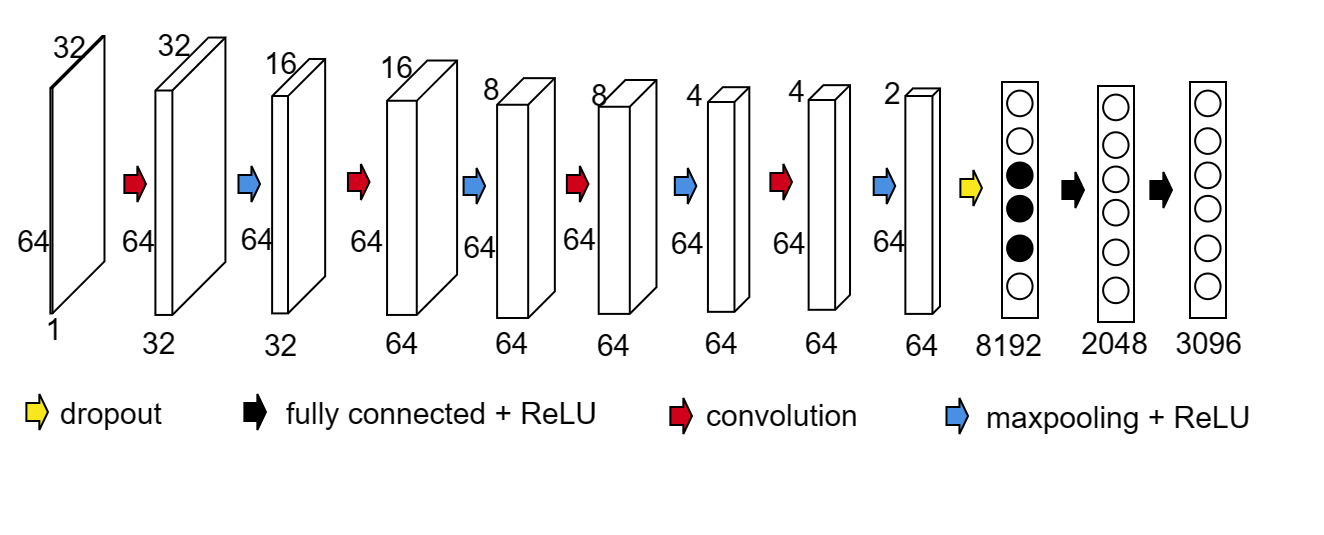
Li et al. [74] proposed using CNN to directly learn the map from the measured data and the conductivity distribution. The employed network architecture is based on LeNet and refined by applying dropout layer and moving average. The CNN architecture used in the numerical experiments below is shown in Fig. 1. Since the number of injected currents and the discretisation size differ from that in [74], we modify the input size, network depth, kernel size, etc. The input size is 32 × 64. The kernel size is 5 × 5 with zero-padding max pooling rather than average pooling is adopted to gain better performance. The sigmoid activation function used in LeNet causes a serious saturation phenomenon, which can lead to vanishing gradients. So, ReLU is chosen as the activation function below. A dropout layer is added to improve the generalisation ability of this model. One-half of the neurons before the first fully connected layers are randomly discarded from the network during the training process. It can reduce the complex co-adaptation among neurons so that the network can learn more robust features. In addition, a dropout layer has been proven to be very effective in training large datasets.
3.4 FC-UNet
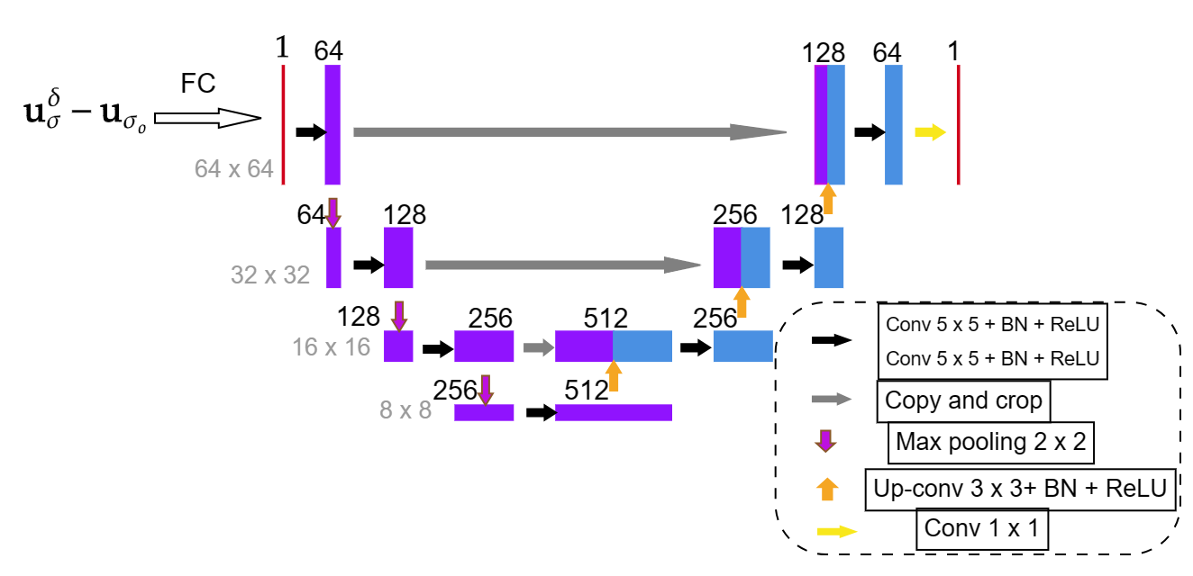
Chen et al. [26] proposed a novel deep learning architecture by adding a fully connected layer before the U-Net structure. The input of the network is given by the difference voltage . Inspired by a linearized approximation of the EIT problem for a small perturbation of conductivity distribution :
| (12) |
where donates the sensitivity matrix, the method first generates an initial guess of the conductivity distribution from the linear fully connected(FC) layer followed by a ReLU layer and then feeds it to a denoising U-Net model to learn the nonlinear relationship further. Thus we could write this process as with and . The authors also proposed an initialisation strategy to further help obtain the initial guess, i.e., the weights of the fully connected layer are initialised with the least-squares solution using training data. The weights for the U-Net are initialised randomly as usual. Then, all weights are updated during the training process. According to the numerical results shown in [26], this special weight initialization strategy can reduce the training time and improve the reconstruction quality. With a trained network, different from the deep D-bar and DDSM methods, the methods FC-UNet and CNN based on LeNet only involve a forward pass of the trained network for each testing example.
Based on our numerical experience, dropping the ReLU layer following the fully connected layer can provide better reconstruction results, at least for the examples in section 4. Thus, for the numerical experiments, we employ the FC-UNet network as shown in Fig. 2, in which only a linear fully connected layer is employed before the U-Net.
In addition, by employing the FC-UNet to extract structure distribution and a standard CNN to extract conductivity values, a structure-aware dual-branch network was designed in [25] to solve EIT problems.
4 Numerical experiments and results
The core of this work is the extensive numerical experiments. Now, we describe how to generate the dataset used in the experiments, highlighting its peculiarity and relevance in real-world scenarios, and also the performance metrics used for comparing different methods. Last, we present and discuss the experimental results.
4.1 Dataset generation and characteristics
Generating simulated data consists of three main parts, which we describe below. The codes for data generation are available at https://github.com/dericknganyu/EIT_dataset_generation.
In the 2D setting, we generate circular phantoms , all restricted to the unit circle centred at the origin, i.e., in the Cartesian coordinates or in polar coordinates. The phantoms are generated randomly. Firstly, we decide on the maximum number of inclusions. Each phantom would then contain inclusions, where , the uniform distribution over the set . To mimic realistic scenarios in medical imaging, the inclusions are elliptical and are sampled such that when , the inclusions do not overlap. Since the inclusions are elliptical, each inclusion, is characterised by a centre , an angle of rotation , a major and minor axis and respectively. The parametric equation of an ellipse is thus given by
| (13) |
To mimic realistic scenarios in medical imaging, the inclusions are sampled to avoid contact with the boundary of the domain . For an inclusion , we have for any . In this way, all phantoms have inclusions contained within . We illustrate this in Algorithm 3.
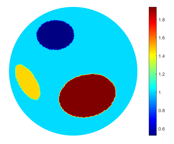
Each phantom has inclusions, with . For each , we assign a conductivity . The background conductivity is set to . In this way, given a point in the domain/phantom, the conductivity at that point is therefore given by
| (14) |
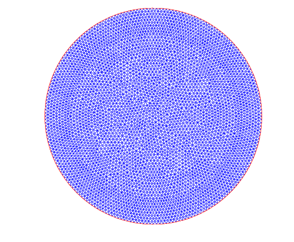
Fig. 3(b) shows an example of a phantom generated in this way.
Next, for any simulated , we solve the forward problem (1) using the Galerkin finite element method (FEM) [71, 39], for the injected currents and in (15) around the boundary . The points are thus nodes in the finite element mesh shown in Fig. 3(a)
| (15) |
We use the MATLAB PDE toolbox in the numerical experiment to solve the forward problem.
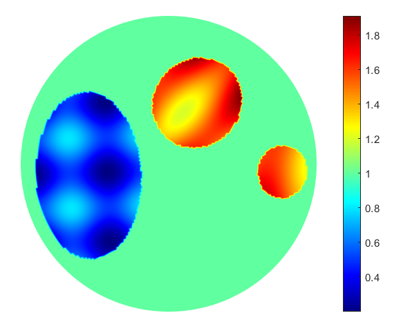
In real-life situations, the conductivities of the inclusions are rarely constant. Indeed, usually, there are textures on internal organs in medical applications. Motivated by this, we take a step further in generating phantoms, with inclusions having variable conductivities. This introduces a novel challenge to the EIT problem, and we seek to study its impact on different reconstruction algorithms. The procedure to generate simulated data remains unchanged. However, in equation (14) becomes
where , is the rotation of centre and angle , with respect to the centre and angle of the ellipse respectively; and applies a scaling so that the resulting is either within the range or . Fig. 3(c) shows an example phantom.
We also study the performance of the methods in noisy scenarios, i.e. reconstructing the conductivity from noisy measurements. The resulting solution to the forward problem , on the boundary , is then perturbed with normally distributed random noise of different levels :
where follows the standard normal distribution .
For the deep learning methods, we employ 20,000 training data and 100 validation data without noises added. Then we compare the results for 100 testing data with different noise levels.
We employ several performance metrics commonly used in the literature to compare different reconstruction methods comprehensively. Table 1 outlines these metrics with their mathematical expressions and specifications. In Table 1, denotes the ground truth with mean and variance , while the predicted conductivity with mean and variance . is the -th element of while is the -th element of . is the total number of pixels, so that and .
| Error Metric | Mathematical Expression | Highlights |
| Relative Image Error (RIE) | Evaluates the relative error between the true value and prediction [26]. | |
| Image Correlation Coefficient (ICC) | Measures the similarity between the true value and prediction[26, 110]. | |
| Dice Coefficient (DC) | Tests the accuracy of the results. It provides a ratio of pixels correctly predicted to the total number of pixels—the closer to 1, the better [41]. For our experiments, we round the pixel values to 2 decimal places before evaluation. | |
| Relative Error (RLE) | Measures the relative difference between the truth and the prediction. The closer to , the better. [41, 110] | |
| Root Mean Squared Error (RMSE) | Evaluates the average magnitude of the differences between the truth and the prediction. [110] | |
| Mean Absolute Error (MAE) | Evaluates the average magnitude of the differences between the truth and the prediction[110] |
4.2 Results and discussions
Tables 2 and 3 present quantitative values for the performance metrics of various EIT reconstruction methods, in the presence of different noise levels, , and, . The considered performance metrics are described in Table 1. Understanding the results requires considering the behaviour of these metrics: For RIE, RMSE, MAE, and RLE, lower values indicate better performance and the objective is to minimise them; for DC and ICC, values closer to 1 indicate better performance, and the goal is to maximise them. Below, we examine the results in each table more closely.
| RIE | ICC | DC | RMSE | MAE | RLE | |
| Sparsity | ||||||
| D-bar | ||||||
| \hdashlineDeep D-bar | ||||||
| DDSM | ||||||
| FC-UNet | ||||||
| CNN LeNet |
| RIE | ICC | DC | RMSE | MAE | RLE | |
| Sparsity | ||||||
| D-bar | ||||||
| \hdashlineDeep D-bar | ||||||
| DDSM | ||||||
| FC-UNet | ||||||
| CNN LeNet |
| RIE | ICC | DC | RMSE | MAE | RLE | |
| Sparsity | ||||||
| D-bar | ||||||
| \hdashlineDeep D-bar | ||||||
| DDSM | ||||||
| FC-UNet | ||||||
| CNN LeNet |
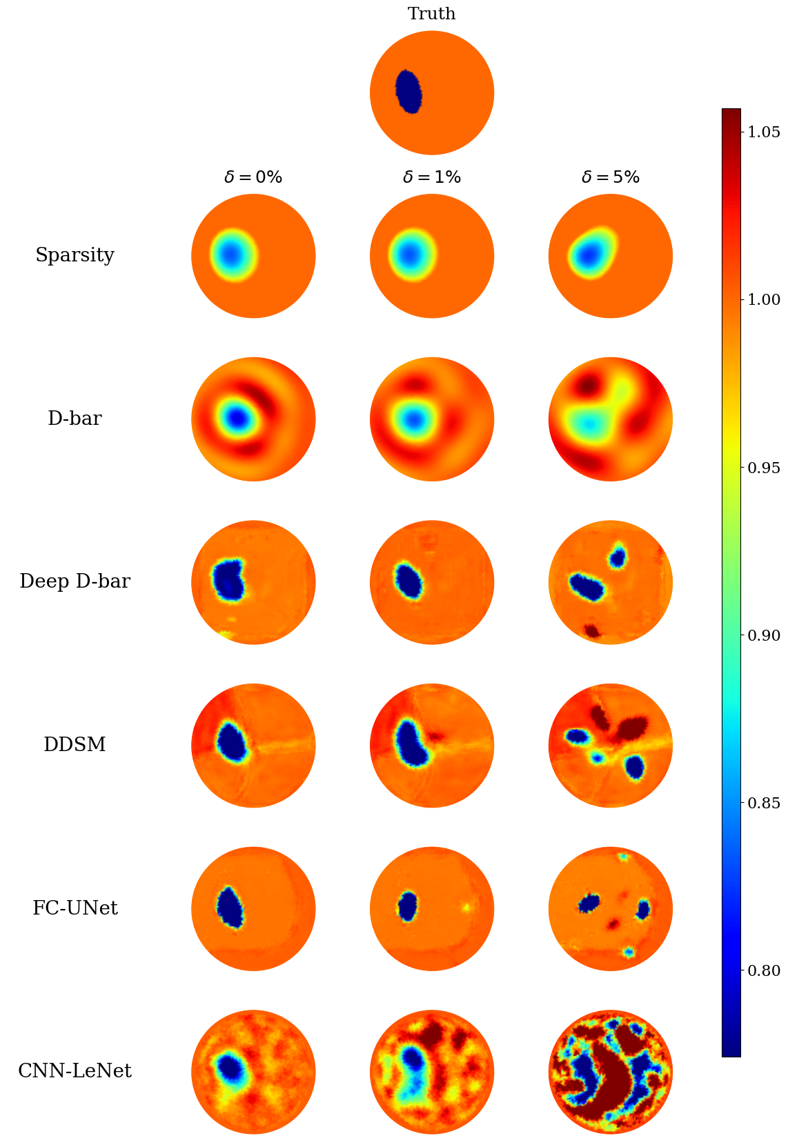
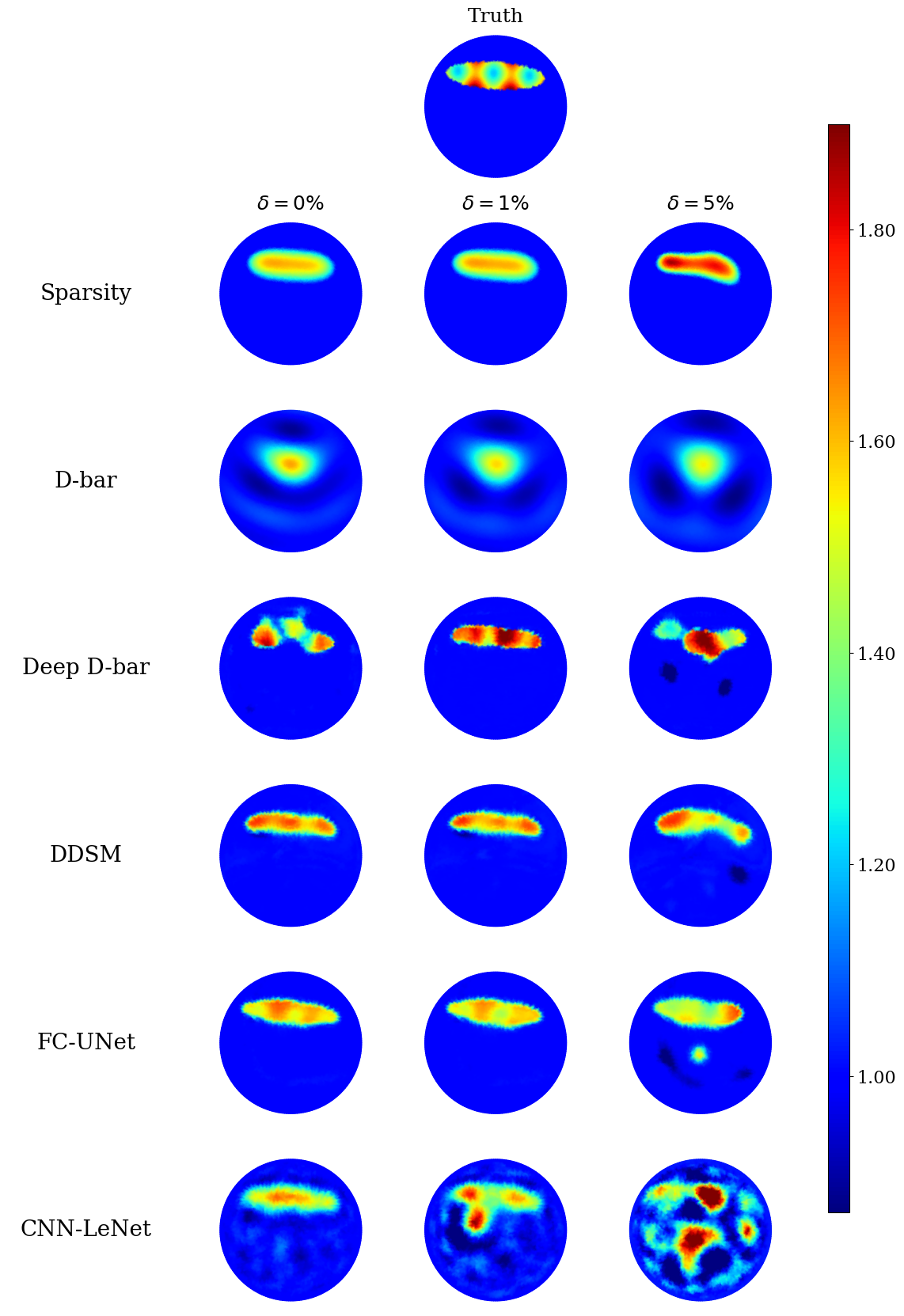
4.2.1 Piece-wise constant conductivities
In the noiseless scenario as depicted in Table 2(a), FC-UNet shows the best performance across all metrics, with notably low RIE, RMSE, MAE, and RLE. It also achieves a high DC and ICC, indicating robustness and accuracy in image reconstruction. The DDSM also performs well, particularly regarding RIE, RMSE, MAE, and RLE. The Deep D-bar method exhibits competitive results, although slightly inferior to FC-UNet. Both Sparsity and D-bar methods show weaker performance compared to the deep learning-based methods. The CNN-LeNet method generally has the worst performance metrics, indicating less accurate image reconstruction.
Under increased noise of , the relative performance of the methods remains consistent, with FC-UNet still demonstrating strong performance. Also, the Deep D-bar performs exceptionally well in this case, particularly in terms of RIE, RMSE, MAE, and RLE. The DDSM also exhibits robust performance under this noise level, while the CNN LeNet method continues to have the highest values for most metrics, indicating challenges in handling noise. In contrast, the analytic-based methods of Sparsity and D-bar show particular robustness to the added noise, evidenced by the unnoticeable change in the performance metrics.
At a higher noise level , the inverse problem becomes more challenging due to the severe ill-posed nature; and in the learned context, since the neural networks are trained on noiseless data, which differ markedly from the noisy data, the setting may be viewed as an out-of-distribution robustness test. Here, the sparsity method comes on top across most metrics, having almost maintained constant performance. However, the FC-UNet continues to maintain the best performance in terms of ICC, emphasising its robustness in noisy conditions. Deep D-bar and DDSM display competitive results, indicating resilience to increased noise. The D-bar methods exhibit slightly weaker performance, especially in terms of RIE, RMSE, and MAE. In contrast, the CNN LeNet method continues to have the highest values for most metrics, suggesting difficulty in coping with substantial noise.
Overall, these results illustrate the varying performance of different EIT methods under different noise levels. The deep learning-based methods, particularly FC-UNet, exhibit good performance across low noise levels. In contrast, the sparsity method shows proof of consistent robustness across higher noise levels, indicating their effectiveness in reconstructing EIT images, even in the presence of noise. Visual results across all the noise levels are shown for two test samples in Figure 4.
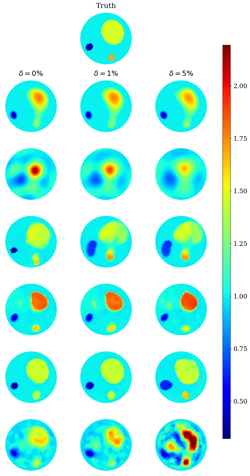
4.2.2 Textured inclusions scenario
In the noiseless scenario depicted in Table 3(a), The best-performing method based on RIE, ICC, RMSE, MAE, and RLE is FC-UNet, with the best values across these metrics. The sparsity method and DDSM also perform well, being the first runners-up in these metrics, particularly for DC; the sparsity method achieves the highest values, indicating good performance, with DDSM as the first runner-up. The worst-performing method across all metrics in this scenario is ”D-bar.”
| RIE | ICC | DC | RMSE | MAE | RLE | |
| Sparsity | ||||||
| D-bar | ||||||
| \hdashlineDeep D-bar | ||||||
| DDSM | ||||||
| FC-UNet | ||||||
| CNN LeNet |
| RIE | ICC | DC | RMSE | MAE | RLE | |
| Sparsity | ||||||
| D-bar | ||||||
| \hdashlineDeep D-bar | ||||||
| DDSM | ||||||
| FC-UNet | ||||||
| CNN LeNet |
| RIE | ICC | DC | RMSE | MAE | RLE | |
| Sparsity | ||||||
| D-bar | ||||||
| \hdashlineDeep D-bar | ||||||
| DDSM | ||||||
| FC-UNet | ||||||
| CNN LeNet |
With a bit of noise of added, the Deep D-bar surprisingly stands out as the best-performing for most of the considered metrics. The FC-UNet closely follows it. The sparsity-based method continues to lead in DC. Like the noiseless scenario, D-bar remains one of the less effective methods across all metrics. This is depicted in Table 3(b).
For higher noise levels in Table 3(c), the sparsity-based methods once again excel in all metrics but for the ICC, making it the best-performing method. The DDSM and FC-UNet closely follow in most of these metrics, while the Deep D-bar continues to perform best in ICC. The CNN LeNet consistently performs the poorest across all metrics and noise levels, especially in this high-noise scenario.
In summary, the best-performing method varies depending on the specific performance metric and noise level. Sparsity consistently demonstrates robust performance in both noiseless and noisy scenarios, while the D-bar is generally less effective. However, in terms of computational expense, the sparsity method is more expensive. The Deep D-bar, FC-UNet, and DDSM often serve as strong contenders, shifting their rankings across noise scenarios and metrics. Meanwhile, CNN LeNet consistently performs the poorest, particularly in high-noise scenarios (). Figure 5 depicts this for two test examples.
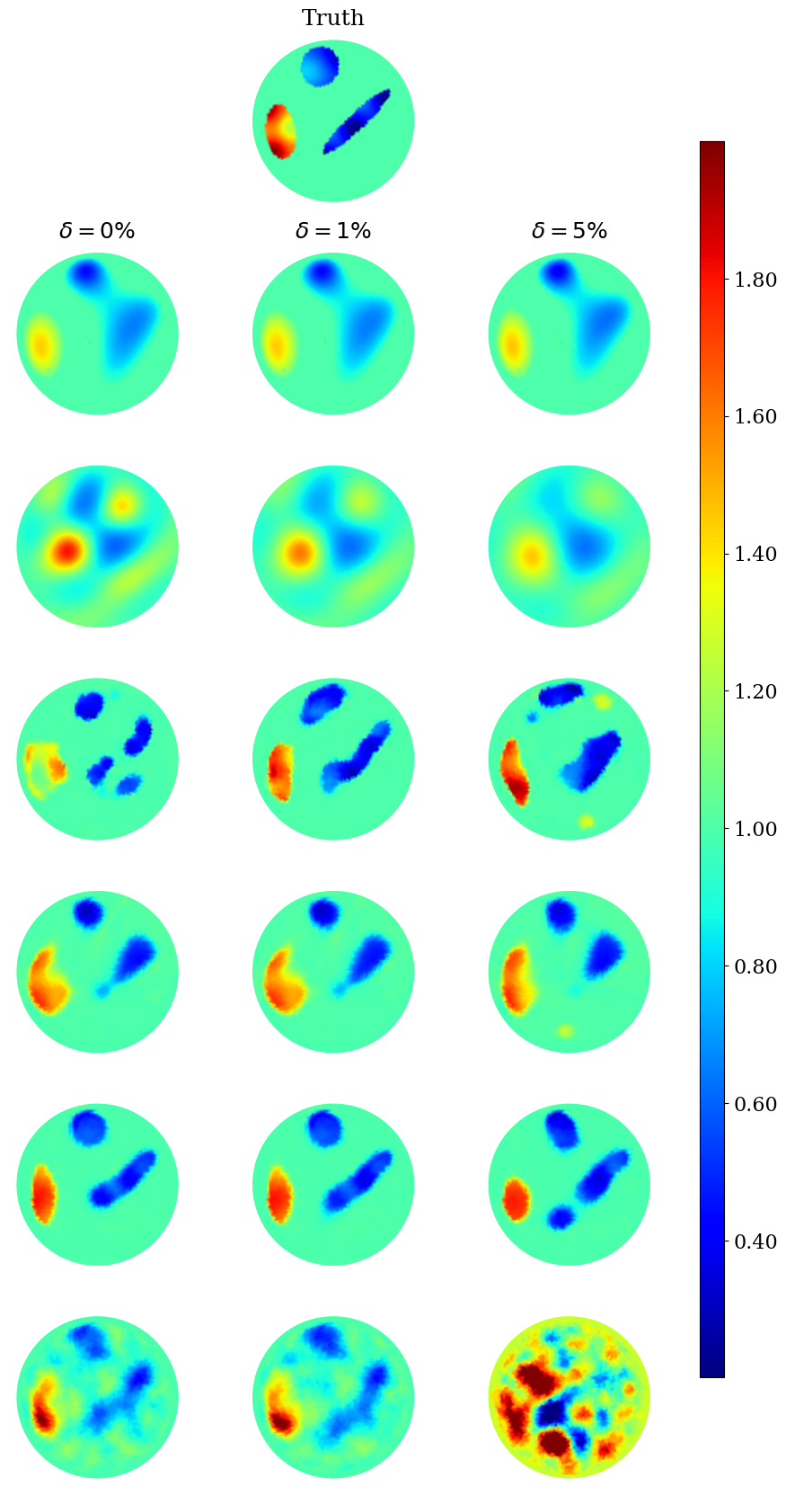
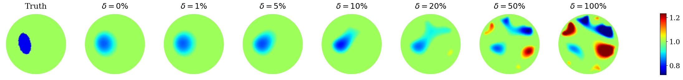
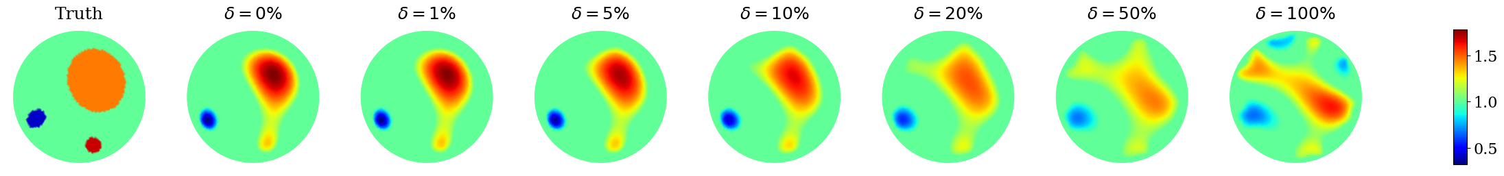
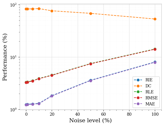
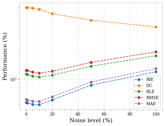
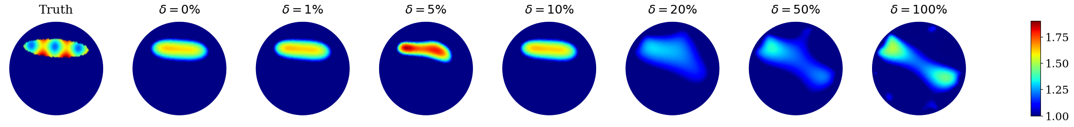
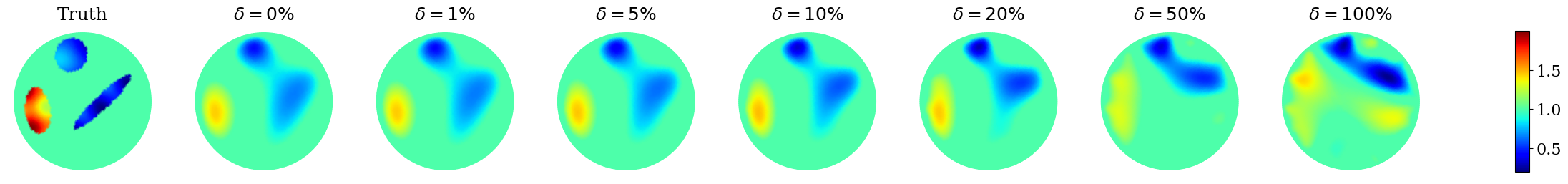
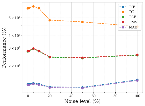
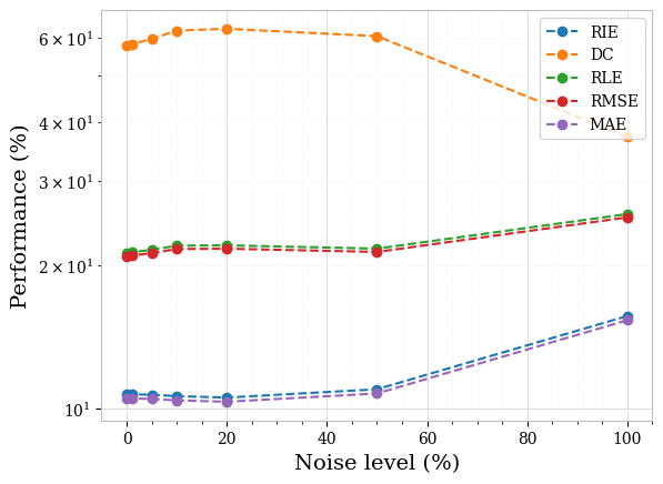
Furthermore, for both piecewise constant and textured phantoms, the sparsity-based method consistently performed well for noisy scenarios. This consistently good performance of the sparsity concept in detecting and locating inclusions even for higher noise levels is most remarkable. The error metrics are almost constant over noise levels up to . Hence, as a side result, we did check the limits of the sparsity concept for very high noise levels, which not surprisingly showed a sharp decrease in the reconstruction accuracy for very high noise levels. We show this in Figure 6, once again for the two piecewise constant samples initially displayed in Figure 4. The respective performances, all metrics considered, for these two samples are equally shown in Figure 7 (ICC is not plotted for the sake of visibility since its values are smallest). Figures 8 and 9 show the corresponding plots for the textured samples initially displayed in Figure 5.
5 Conclusion and future directions
In summary, this review has comprehensively examined numerical methods for addressing the EIT inverse problem. EIT, a versatile imaging technique with applications in various fields, presents a highly challenging task of reconstructing internal conductivity distributions from boundary measurements. We explored the interplay between modern deep learning-based approaches and traditional analytic methods for solving the EIT inverse problem. Four advanced deep learning algorithms were rigorously assessed, including the deep D-bar method, deep direct sampling method, fully connected U-net, and convolutional neural networks. Additionally, two analytic-based methods, incorporating mathematical formulations and regularisation techniques, were examined regarding their efficacy and limitations. Our evaluation involved a comprehensive array of numerical experiments encompassing diverse scenarios that mimic real-world complexities. Multiple performance metrics were employed to shed insights into the methods’ capabilities to capture essential features and delineate complex conductivity patterns.
The first evaluation was based on piecewise constant conductivities. The clear winners of this series of tests are the analytic sparsity-based reconstruction and the learned FC-UNet. Both perform best, with slight variations depending on the noise level. This is not surprising for learned methods, which adapt well to this particular set of test data. However, the excellent performance of sparsity methods, which can identify and locate piecewise constant inclusions correctly, is most remarkable.
A noteworthy aspect of this study was the introduction of variable conductivity scenarios, mimicking textured inclusions and departing from uniform conductivity assumptions. This enabled us to assess how each method responds to varying conductivity, shedding light on their robustness and adaptability. Here, the D-bar with learned post-processing achieves competitive results. The winning algorithm alternates between sparsity, Deep D-bar and FC-UNet. The good performance of the sparsity concepts is somewhat surprising for these textured test samples. However, none of the proposed methods was able to reconstruct the textures reliably for higher noise levels. That is, the quality of the reconstruction was mainly measured in terms of how well the inclusions were located - which gives a particular advantage to sparsity concepts.
These results naturally raise questions about the numerical results presented in several existing EIT studies, where learned methods were only compared with sub-optimal analytic methods. Our findings clearly indicate that at least within the restricted scope of the present study, optimised analytical methods can reach a comparable or even superior accuracy. Of course, one should note that after training, learned methods are much more efficient and provide a preferred option for real-time imaging.
In conclusion, this review contributes to a deeper understanding of the available solutions for the EIT inverse problem, highlighting the role of deep learning and analytic-based methods in advancing the field.
Acknowledgements
D.N.T. acknowledges the financial support of this research work within the Research Unit 3022 ”Ultrasonic Monitoring of Fiber Metal Laminates Using Integrated Sensors” by the German Research Foundation (Deutsche Forschungsgemeinschaft (DFG)) under grant number LO1436/12-1 and project number 418311604.
J.N. acknowledges the financial support from the program of China Scholarships Council (No. 202006270155).
A.H. acknowledges support by the Research Council of Finland: Academy Research Fellow (Project No. 338408) and the Centre of Excellence of Inverse Modelling and Imaging project (Project No. 353093).
B.J. acknowledges the support by a start-up fund and Direct Grant of Research, both from The Chinese University of Hong Kong, Hong Kong General Research Fund (Project No. 14306423) and UK Engineering and Physical Research Council (EP/V026259/1).
P.M. acknowledges the financial support from the DFG project number 281474342: Graduiertenkolleg RTG 2224 Parameter Identification - Analysis, Algorithms, Applications.
References
- [1] G. Alessandrini. Stable determination of conductivity by boundary measurements. Applicable Analysis, 27(1-3):153–172, 1988.
- [2] H. Ammari, R. Griesmaier, and M. Hanke. Identification of small inhomogeneities: asymptotic factorization. Math. Comp., 76(259):1425–1448, 2007.
- [3] H. Ammari, E. Iakovleva, and D. Lesselier. A MUSIC algorithm for locating small inclusions buried in a half-space from the scattering amplitude at a fixed frequency. Multiscale Model. Simul., 3(3):597–628, 2005.
- [4] V. Antun, F. Renna, C. Poon, and A. C. Hansen. On instabilities of deep learning in image reconstruction and the potential costs of AI. Proc. Nat. Acad. Sci., 117(48):30088–30095, 2020.
- [5] S. Arridge, P. Maass, O. Öktem, and C.-B. Schönlieb. Solving inverse problems using data-driven models. Acta Numer., 28:1–174, 2019.
- [6] K. Astala, D. Faraco, and L. Székelyhidi, Jr. Convex integration and the theory of elliptic equations. Ann. Sc. Norm. Super. Pisa Cl. Sci. (5), 7(1):1–50, 2008.
- [7] K. Astala and L. Päivärinta. Calderón’s inverse conductivity problem in the plane. Ann. of Math. (2), 163(1):265–299, 2006.
- [8] G. Bao, X. Ye, Y. Zang, and H. Zhou. Numerical solution of inverse problems by weak adversarial networks. Inverse Problems, 36(11):115003, 2020.
- [9] L. Bar and N. Sochen. Strong solutions for pde-based tomography by unsupervised learning. SIAM J. Imag. Sci., 14(1):128–155, 2021.
- [10] J. Barzilai and J. M. Borwein. Two-point step size gradient methods. IMA J. Numer. Anal., 8(1):141–148, 1988.
- [11] J. Bikowski and J. L. Mueller. 2D EIT reconstructions using Calderón’s method. Inverse Probl. Imaging, 2(1):43–61, 2008.
- [12] J. Bohr. A Bernstein–von-Mises theorem for the Calderón problem with piecewise constant conductivities. Inverse Problems, 39(1):015002, 18, 2023.
- [13] T. Bonesky, K. Bredies, D. A. Lorenz, and P. Maass. A generalized conditional gradient method for nonlinear operator equations with sparsity constraints. Inverse Problems, 23(5):2041–2058, 2007.
- [14] L. Borcea. Electrical impedance tomography. Inverse Problems, 18(6):R99–R136, 2002.
- [15] L. Borcea, G. A. Gray, and Y. Zhang. Variationally constrained numerical solution of electrical impedance tomography. Inverse Problems, 19(5):1159–1184, 2003.
- [16] A. Borsic, B. M. Graham, A. Adler, and W. R. B. Lionheart. In vivo impedance imaging with total variation regularization. IEEE Trans. Med. Imag., 29(1):44–54, 2010.
- [17] K. Bredies, D. A. Lorenz, and P. Maass. A generalized conditional gradient method and its connection to an iterative shrinkage method. Comput. Optim. Appl., 42(2):173–193, 2009.
- [18] M. Brühl and M. Hanke. Numerical implementation of two noniterative methods for locating inclusions by impedance tomography. Inverse Problems, 16(4):1029–1042, 2000.
- [19] M. Brühl, M. Hanke, and M. S. Vogelius. A direct impedance tomography algorithm for locating small inhomogeneities. Numer. Math., 93(4):635–654, 2003.
- [20] A.-P. Calderón. On an inverse boundary value problem. In Seminar on Numerical Analysis and its Applications to Continuum Physics (Rio de Janeiro, 1980), pages 65–73. Soc. Brasil. Mat., Rio de Janeiro, 1980.
- [21] S. Cen, B. Jin, K. Shin, and Z. Zhou. Electrical impedance tomography with deep Calderon method. J. Comput. Phys., 493:112427, 2023.
- [22] S. Chaabane, C. Elhechmi, and M. Jaoua. Error estimates in smoothing noisy data using cubic B-splines. C. R. Math. Acad. Sci. Paris, 346(1-2):107–112, 2008.
- [23] Z. Chen, Z. Liu, L. Ai, S. Zhang, and Y. Yang. Mask-guided spatial–temporal graph neural network for multifrequency electrical impedance tomography. IEEE Trans. Instrum. Meas., 71:4505610, 2022.
- [24] Z. Chen, J. Xiang, P.-O. Bagnaninchi, and Y. Yang. MMV-Net: A multiple measurement vector network for multifrequency electrical impedance tomography. IEEE Trans. Neural Networks Learn. System, page in press, 2022.
- [25] Z. Chen and Y. Yang. Structure-aware dual-branch network for electrical impedance tomography in cell culture imaging. IEEE Trans. Instrum. Meas., 70:1–9, 2021.
- [26] Z. Chen, Y. Yang, J. Jia, and P. Bagnaninchi. Deep learning based cell imaging with electrical impedance tomography. In 2020 IEEE International Instrumentation and Measurement Technology Conference (I2MTC), pages 1–6, 2020.
- [27] M. Cheney and D. Isaacson. Distinguishability in impedance imaging. IEEE Trans. Biomed. Imag., 39(8):852–860, 1992.
- [28] M. Cheney, D. Isaacson, J. C. Newell, S. Simske, and J. Goble. NOSER: An algorithm for solving the inverse conductivity problem. Int. J. Imag. Syst. Tech., 2:66–75, 1990.
- [29] Y. T. Chow, K. Ito, and J. Zou. A direct sampling method for electrical impedance tomography. Inverse Problems, 30(9):095003, 2014.
- [30] E. T. Chung, T. F. Chan, and X.-C. Tai. Electrical impedance tomography using level set representation and total variational regularization. J. Comput. Phys., 205(1):357–372, 2005.
- [31] F. Colibazzi, D. Lazzaro, S. Morigi, and A. Samoré. Deep-plug-and-play proximal gauss-newton method with applications to nonlinear, ill-posed inverse problems. Inverse Probl. Imaging, pages 0–0, 2023.
- [32] Y.-H. Dai, W. W. Hager, K. Schittkowski, and H. Zhang. The cyclic Barzilai-Borwein method for unconstrained optimization. IMA J. Numer. Anal., 26(3):604–627, 2006.
- [33] I. Daubechies, M. Defrise, and C. De Mol. An iterative thresholding algorithm for linear inverse problems with a sparsity constraint. Comm. Pure Appl. Math., 57(11):1413–1457, 2004.
- [34] M. M. Dunlop and A. M. Stuart. The Bayesian formulation of EIT: analysis and algorithms. Inverse Probl. Imaging, 10(4):1007–1036, 2016.
- [35] H. W. Engl, M. Hanke, and A. Neubauer. Regularization of inverse problems. Kluwer Academic Publishers Group, Dordrecht, 1996.
- [36] L. D. Faddeev. Increasing solutions of the Schrödinger equation. Sov.-Phys. Dokl., 10:1033–5, 1966.
- [37] Y. Fan and L. Ying. Solving electrical impedance tomography with deep learning. J. Comput. Phys., 404:109119, 2020.
- [38] M. Gehre and B. Jin. Expectation propagation for nonlinear inverse problems–with an application to electrical impedance tomography. J. Comput. Phys., 259:513–535, 2014.
- [39] M. Gehre, B. Jin, and X. Lu. An analysis of finite element approximation in electrical impedance tomography. Inverse Problems, 30(4):045013, 2014.
- [40] M. Gehre, T. Kluth, A. Lipponen, B. Jin, A. Seppänen, J. P. Kaipio, and P. Maass. Sparsity reconstruction in electrical impedance tomography: an experimental evaluation. J. Comput. Appl. Math., 236(8):2126–2136, 2012.
- [41] R. Guo, S. Cao, and L. Chen. Transformer meets boundary value inverse problems. In The Twelfth International Conference on Learning Representations, 2023.
- [42] R. Guo and J. Jiang. Construct deep neural networks based on direct sampling methods for solving electrical impedance tomography. SIAM J. Sci. Comput., 43(3):B678–B711, 2021.
- [43] R. Guo, J. Jiang, and Y. Li. Learn an index operator by cnn for solving diffusive optical tomography: A deep direct sampling method. J. Sci. Comput., 95(1):31, 2023.
- [44] S. J. Hamilton, A. Hänninen, A. Hauptmann, and V. Kolehmainen. Beltrami-net: domain-independent deep d-bar learning for absolute imaging with electrical impedance tomography (a-EIT). Physiol. Meas., 40(7):074002, 2019.
- [45] S. J. Hamilton and A. Hauptmann. Deep D-bar: Real-time electrical impedance tomography imaging with deep neural networks. IEEE Trans. Med. Imag., 37(10):2367–2377, 2018.
- [46] S. J. Hamilton, A. Hauptmann, and S. Siltanen. A data-driven edge-preserving D-bar method for electrical impedance tomography. Inverse Probl. Imaging, 8(4):1053–1072, 2014.
- [47] B. Harrach and M. Ullrich. Monotonicity-based shape reconstruction in electrical impedance tomography. SIAM J. Math. Anal., 45(6):3382–3403, 2013.
- [48] W. Herzberg, A. Hauptmann, and S. J. Hamilton. Domain independent post-processing with graph u-nets: Applications to electrical impedance tomographic imaging. arXiv preprint arXiv:2305.05020, 2023.
- [49] W. Herzberg, D. B. Rowe, A. Hauptmann, and S. J. Hamilton. Graph convolutional networks for model-based learning in nonlinear inverse problems. IEEE Trans. Comput. Imag., 7:1341–1353, 2021.
- [50] M. Hinze, B. Kaltenbacher, and T. N. T. Quyen. Identifying conductivity in electrical impedance tomography with total variation regularization. Numer. Math., 138(3):723–765, 2018.
- [51] D. S. Holder, editor. Electrical Impedance Tomography: Methods, History and Applications. Institute of Physics Publishing, Bristol, 2004.
- [52] S.-W. Huang, H.-M. Cheng, and S.-F. Lin. Improved imaging resolution of electrical impedance tomography using artificial neural networks for image reconstruction. In 2019 41st Annual International Conference of the IEEE Engineering in Medicine and Biology Society (EMBC), pages 1551–1554. IEEE, 2019.
- [53] N. Hyvönen. Complete electrode model of electrical impedance tomography: approximation properties and characterization of inclusions. SIAM J. Appl. Math., 64(3):902–931, 2004.
- [54] M. Ikehata. Size estimation of inclusion. J. Inverse Ill-Posed Probl., 6(2):127–140, 1998.
- [55] V. Isakov. Inverse Problems for Partial Differential Equations. Springer, New York, 2nd edition, 2006.
- [56] K. Ito and B. Jin. Inverse problems: Tikhonov theory and algorithms. World Scientific Publishing Co. Pte. Ltd., Hackensack, NJ, 2015.
- [57] B. Jin, T. Khan, P. Maass, and M. Pidcock. Function spaces and optimal currents in impedance tomography. J. Inverse Ill-Posed Probl., 19(1):25–48, 2011.
- [58] B. Jin and P. Maass. An analysis of electrical impedance tomography with applications to tikhonov regularization. ESAIM: Control, Optim. Cal. Var., 18(4):1027–1048, 2012.
- [59] B. Jin and P. Maass. Sparsity regularization for parameter identification problems. Inverse Problems, 28(12):123001, nov 2012.
- [60] B. Jin, P. Maass, and O. Scherzer. Sparsity regularization in inverse problems. Inverse Problems, 33(6):060301, 2017.
- [61] B. Jin and Y. Xu. Adaptive reconstruction for electrical impedance tomography with a piecewise constant conductivity. Inverse Problems, 36(1):014003, 2019.
- [62] B. Jin, Y. Xu, and J. Zou. A convergent adaptive finite element method for electrical impedance tomography. IMA J. Numer. Anal., 37(3):1520–1550, 2017.
- [63] K. H. Jin, M. T. McCann, E. Froustey, and M. Unser. Deep convolutional neural network for inverse problems in imaging. IEEE Trans. Image Proc., 26(9):4509–4522, 2017.
- [64] J. P. Kaipio, V. Kolehmainen, E. Somersalo, and M. Vauhkonen. Statistical inversion and Monte Carlo sampling methods in electrical impedance tomography. Inverse Problems, 16(5):1487–1522, 2000.
- [65] T. A. Khan and S. H. Ling. Review on electrical impedance tomography: Artificial intelligence methods and its applications. Algorithms, 12(5):88, 2019.
- [66] D. P. Kingma and J. Ba. Adam: A method for stochastic optimization. In 3rd International Conference for Learning Representations, San Diego, 2015.
- [67] I. Knowles. A variational algorithm for electrical impedance tomography. Inverse Problems, 14(6):1513–1525, 1998.
- [68] K. Knudsen, M. Lassas, J. L. Mueller, and S. Siltanen. Regularized D-bar method for the inverse conductivity problem. Inverse Probl. Imaging, 3(4):599–624, 2009.
- [69] R. V. Kohn and A. McKenney. Numerical implementation of a variational method for electrical impedance tomography. Inverse Problems, 6(3):389–414, 1990.
- [70] A. Lechleiter. The MUSIC algorithm for impedance tomography of small inclusions from discrete data. Inverse Problems, 31(9):095004, 19, 2015.
- [71] A. Lechleiter and A. Rieder. Newton regularizations for impedance tomography: a numerical study. Inverse Problems, 22(6):1967–1987, 2006.
- [72] A. Lechleiter and A. Rieder. Newton regularizations for impedance tomography: convergence by local injectivity. Inverse Problems, 24(6):065009, 18, 2008.
- [73] X. Li, R. Lu, Q. Wang, J. Wang, X. Duan, Y. Sun, X. Li, and Y. Zhou. One-dimensional convolutional neural network (1d-cnn) image reconstruction for electrical impedance tomography. Rev. Sci. Instrument., 91(12), 2020.
- [74] X. Li, Y. Lu, J. Wang, X. Dang, Q. Wang, X. Duan, and Y. Sun. An image reconstruction framework based on deep neural network for electrical impedance tomography. In 2017 IEEE International Conference on Image Processing (ICIP), pages 3585–3589. IEEE, 2017.
- [75] Z. Li, N. Kovachki, K. Azizzadenesheli, B. Liu, K. Bhattacharya, A. Stuart, and A. Anandkumar. Fourier neural operator for parametric partial differential equations. arXiv preprint arXiv:2010.08895, 2020.
- [76] D. Liu, J. Wang, Q. Shan, D. Smyl, J. Deng, and J. Du. Deepeit: deep image prior enabled electrical impedance tomography. IEEE Trans. Pattern Anal. Mach. Intell., 45(8):9627–9638, 2023.
- [77] L. Lu, P. Jin, G. Pang, Z. Zhang, and G. E. Karniadakis. Learning nonlinear operators via deeponet based on the universal approximation theorem of operators. Nature Mach. Int., 3(3):218–229, 2021.
- [78] M. Lukaschewitsch, P. Maass, and M. Pidcock. Tikhonov regularization for electrical impedance tomography on unbounded domains. Inverse Problems, 19(3):585–610, 2003.
- [79] S. Martin and C. T. Choi. A post-processing method for three-dimensional electrical impedance tomography. Sci. Rep., 7(1):7212, 2017.
- [80] N. G. Meyers. An e-estimate for the gradient of solutions of second order elliptic divergence equations. Ann. Scuola Norm. Sup. Pisa Cl. Sci. (3), 17:189–206, 1963.
- [81] V. Monga, Y. Li, and Y. C. Eldar. Algorithm unrolling: interpretable, efficient deep learning for signal and image processing. IEEE Signal Proc. Magaz., 38(2):18–44, 2021.
- [82] J. L. Mueller and S. Siltanen. The D-bar method for electrical impedance tomography—demystified. Inverse Problems, 36(9):093001, 28, 2020.
- [83] A. I. Nachman. Global uniqueness for a two-dimensional inverse boundary value problem. Ann. of Math. (2), 143(1):71–96, 1996.
- [84] J. W. Neuberger. Sobolev gradients and differential equations, volume 1670 of Lecture Notes in Mathematics. Springer-Verlag, Berlin, 1997.
- [85] D. Nganyu Tanyu, J. Ning, T. Freudenberg, N. Heilenkoetter, A. Rademacher, U. Iben, and P. Maass. Deep learning methods for partial differential equations and related parameter identification problems. Inverse Problems, 39(10):103001, aug 2023.
- [86] J. Ning, F. Han, and J. Zou. A direct sampling-based deep learning approach for inverse medium scattering problems. arXiv preprint arXiv:2305.00250, 2023.
- [87] R. G. Novikov. A multidimensional inverse spectral problem for the equation . Funktsional. Anal. i Prilozhen., 22(4):11–22, 96, 1988.
- [88] A. Pokkunuru, P. Rooshenas, T. Strauss, A. Abhishek, and T. Khan. Improved training of physics-informed neural networks using energy-based priors: a study on electrical impedance tomography. In The Eleventh International Conference on Learning Representations, 2022.
- [89] M. Raissi, P. Perdikaris, and G. E. Karniadakis. Physics-informed neural networks: A deep learning framework for solving forward and inverse problems involving nonlinear partial differential equations. J. Comput. Phys., 378:686–707, 2019.
- [90] S. Ren, R. Guan, G. Liang, and F. Dong. RCRC: A deep neural network for dynamic image reconstruction of electrical impedance tomography. IEEE Trans. Instrum. Meas., 70:1–11, 2021.
- [91] L. Rondi. Discrete approximation and regularisation for the inverse conductivity problem. Rend. Istit. Mat. Univ. Trieste, 48:315–352, 2016.
- [92] L. Rondi and F. Santosa. Enhanced electrical impedance tomography via the Mumford-Shah functional. ESAIM Control Optim. Calc. Var., 6:517–538, 2001.
- [93] O. Ronneberger, P. Fischer, and T. Brox. U-net: Convolutional networks for biomedical image segmentation. In Medical Image Computing and Computer-Assisted Intervention–MICCAI 2015: 18th International Conference, Munich, Germany, October 5-9, 2015, Proceedings, Part III 18, pages 234–241. Springer, 2015.
- [94] T. Schuster, B. Kaltenbacher, B. Hofmann, and K. S. Kazimierski. Regularization methods in Banach spaces. Walter de Gruyter GmbH & Co. KG, Berlin, 2012.
- [95] J. Seo, K. Kim, A. Jargal, K. Lee, and B. Harrach. A learning-based method for solving ill-posed nonlinear inverse problems: A simulation study of lung eit. SIAM Journal on Imaging Sciences, 12(3):1275–1295, 2019.
- [96] K. Shin and J. L. Mueller. A second order Calderón’s method with a correction term and a priori information. Inverse Problems, 36(12):124005, 22, 2020.
- [97] S. Siltanen and T. Ide. Electrical impedance tomography, enclosure method and machine learning. In 2020 IEEE 30th International Workshop on Machine Learning for Signal Processing (MLSP), pages 1–6. IEEE, 2020.
- [98] S. Siltanen, J. Mueller, and D. Isaacson. An implementation of the reconstruction algorithm of A. Nachman for the 2D inverse conductivity problem. Inverse Problems, 16(3):681–699, 2000.
- [99] D. Smyl, T. N. Tallman, D. Liu, and A. Hauptmann. An efficient quasi-newton method for nonlinear inverse problems via learned singular values. IEEE Signal Processing Letters, 28:748–752, 2021.
- [100] E. Somersalo, M. Cheney, and D. Isaacson. Existence and uniqueness for electrode models for electric current computed tomography. SIAM J. Appl. Math., 52(4):1023–1040, 1992.
- [101] B. Sun, H. Zhong, Y. Zhao, L. Ma, and H. Wang. Calderón’s method-guided deep neural network for electrical impedance tomography. IEEE Trans. Instrum. Meas., page in press, 2023.
- [102] C. Tan, S. Lv, F. Dong, and M. Takei. Image reconstruction based on convolutional neural network for electrical resistance tomography. IEEE Sensors J., 19(1):196–204, 2018.
- [103] T. Tripura and S. Chakraborty. Wavelet neural operator: a neural operator for parametric partial differential equations. arXiv preprint arXiv:2205.02191, 2022.
- [104] G. Uhlmann. Electrical impedance tomography and Calderón’s problem. Inverse Problems, 25(12):123011, 39, 2009.
- [105] D. Ulyanov, A. Vedaldi, and V. Lempitsky. Deep image prior. In Proceedings of the IEEE Conference on Computer Vision and Pattern Recognition, pages 9446–9454, 2018.
- [106] Z. Wei, D. Liu, and X. Chen. Dominant-current deep learning scheme for electrical impedance tomography. IEEE Trans. Biomed. Eng., 66(9):2546–2555, 2019.
- [107] A. Wexler, B. Fry, and N. M. Impedance-computed tomography algorithm and system. Appl. Opt., 25:3985–92, 1985.
- [108] S. J. Wright, R. D. Nowak, and M. A. T. Figueiredo. Sparse reconstruction by separable approximation. IEEE Trans. Signal Process., 57(7):2479–2493, 2009.
- [109] Y. Wu, B. Chen, K. Liu, C. Zhu, H. Pan, J. Jia, H. Wu, and J. Yao. Shape reconstruction with multiphase conductivity for electrical impedance tomography using improved convolutional neural network method. IEEE Sensors J., 21(7):9277–9287, 2021.
- [110] D. Yang, S. Li, Y. Zhao, B. Xu, and W. Tian. An eit image reconstruction method based on densenet with multi-scale convolution. Math. Biosci. Eng., 20(4):7633–7660, 2023.
- [111] X. Zhang, Z. Wang, R. Fu, D. Wang, X. Chen, X. Guo, and H. Wang. V-shaped dense denoising convolutional neural network for electrical impedance tomography. IEEE Trans. Instrum. Meas., 71:1–14, 2022.
- [112] Z. Zhou, G. S. dos Santos, T. Dowrick, J. Avery, Z. Sun, H. Xu, and D. S. Holder. Comparison of total variation algorithms for electrical impedance tomography. Physiol. Meas., 36(6):1193–1209, 2015.