Electromagnetic waves destabilized by runaway electrons in near-critical electric fields
Abstract
Runaway electron distributions are strongly anisotropic in velocity space. This anisotropy is a source of free energy that may destabilize electromagnetic waves through a resonant interaction between the waves and the energetic electrons. In this work we investigate the high-frequency electromagnetic waves that are destabilized by runaway electron beams when the electric field is close to the critical field for runaway acceleration. Using a runaway electron distribution appropriate for the near-critical case we calculate the linear instability growth rate of these waves and conclude that the obliquely propagating whistler waves are most unstable. We show that the frequencies, wave numbers and propagation angles of the most unstable waves depend strongly on the magnetic field. Taking into account collisional and convective damping of the waves, we determine the number density of runaways that is required to destabilize the waves and show its parametric dependences.
I Introduction
Relativistic runaway electron populations have been frequently observed in various plasmas, e.g. large tokamak disruptions td , electric discharges associated with thunderstorms tavani and solar flares moghaddam . Runaway electrons are produced when the electric field is larger than a certain critical field (), and the accelerating force overwhelms the friction for high energy electrons. The anisotropy of the runaway electron distribution can lead to destabilization of electromagnetic waves through wave-particle resonant interaction. Several studies have shown that the velocity anisotropy excites electromagnetic waves mainly through the anomalous Doppler resonance fulop ; pokol . Once the instability is triggered the distribution is isotropized due to pitch-angle scattering. Previous work pokol ; fulop ; fulop1 has considered whistler wave instability driven by an anisotropic electron distribution as a possible cause for the observed magnetic field threshold for runaway generation in large tokamaks gill ; jt60 . These calculations relied on a distribution function that was based on an approximate solution of the kinetic equation in the case when the electric field is well above the critical field, , where
| (1) |
where is the thermal electron density, is the electron rest mass, is the electron charge, is the Coulomb logarithm, is the dielectric constant and is the speed of light. Also, in many studies, the runaway electrons were assumed to be ultra-relativistic (velocities within to the speed of light) and simplified resonance conditions were used to describe the wave-particle interaction. However, the electric field is not always much larger than the critical field and the velocity of the electrons is often not that close to the speed of light. An example of this is the observations of superthermal electron populations in the T-10 tokamak during magnetic reconnection events, when the electric field was transiently larger than the critical field during the reconnection (for about ) but then it dropped to values near or even below the critical field savrukhin . Recent work riemann has shown that even in disruptions the electric field in the core region of the plasma is only slightly above the critical electric field, .
The purpose of this work is to determine what waves could be destabilized by runaway beams in a near-critical field. Investigating the lowest relevant limit of the electric field when runaway production occurs is a step toward generalizing the analysis of the runaway electron driven instabilities to lower electric fields. This way we can gain confidence that the analysis of the wave-particle interaction yields valid results in both the high electric field and the near-critical limit, before proceeding to the numerical analysis of the interaction for electric fields in between.
In the present work we use the runaway distribution derived in Reference sandquist , appropriate for a near-critical field, to calculate the instability growth rate of these waves and determine the frequencies and wave numbers of the most unstable waves for various parameters. We use a general resonance condition, without the ultra-relativistic assumption, so the model can be applied also for electrons with lower energies. We show that the whistler branch is destabilized via the anomalous Doppler and Cherenkov resonances. Increasing magnetic field leads to increasing wave number and frequency while decreasing propagation angle for the most unstable wave. The observation of these waves could help to determine the origin and evolution of the energetic electrons. If the waves grow to significant amplitude they may contribute to efficient transport of particles out from the plasma.
The remainder of the paper is organized as follows. In Sec. II, the wave dispersion equation is presented, together with a perturbative approximation of the instability growth rate. In Sec. III the runaway electron distribution in a near-critical electric field is analyzed and the runaway contribution to the susceptibilities is calculated. In Sec. IV the instability growth rate of the high-frequency electromagnetic waves driven by runaways is calculated and the parameters of the most unstable wave are determined. Here, we also show the stability thresholds of the waves and study their parametric dependences. Finally, the results are summarized and discussed in Sec. V.
II Dispersion relation
The dispersion relation of high frequency electromagnetic waves is given by stix
| (2) |
where is the wave frequency, k the wave number and the dielectric tensor of the plasma. Equation (2) follows from the wave-equation, with the approximation , where is a dimensionless vector with the magnitude of the refractive index, , is the pitch angle. The subscripts ∥ and ⟂ denote the parallel and perpendicular directions with respect to the magnetic field. The dielectric tensor is
| (3) |
where is the susceptibility of plasma species , where denotes the ion, the thermal electron and the runaway electron populations, 1 is the dyadic unit. As the contribution of the runaway population is expected to be small, we consider the dispersion of high frequency electromagnetic waves without the runaway term and use the cold plasma approximation stix for the ion and electron populations. The contribution of runaway electrons is added later as a perturbation, which is justified in the present case since the runaway electron density is much smaller than the thermal electron and ion density.
II.1 Electron-whistler wave
For the frequency range , the background ion and electron contributions to are stix
| (4) |
Here and are the electron plasma and cyclotron frequencies, respectively. Without runaways, the dispersion relation can be written as
| (5) |
Equation (5) has three solutions for and these can be determined analytically, although their closed form expressions are very complicated. One of the solutions satisfies for all wave numbers and propagation angles and will be called ‘electron-whistler’ wave, because in certain limits, as we will show, its dispersion characteristics are the same as the whistler wave’s. For the two other solutions is satisfied. For typical experimental parameters, the solution of the analytical dispersion relation (5) has excellent agreement with the numerical solution of the full dispersion relation using the hot plasma susceptibilities for both ions and electrons from Reference stix instead of Equation (4). Figure 1a shows the three solutions of Equation (5) together with the solution of the numerical dispersion relation. The solution for the wave frequency is plotted as function of wave number for propagation angle . The wave dispersions in Figure 1 are calculated for . The agreement is even better at lower temperatures.
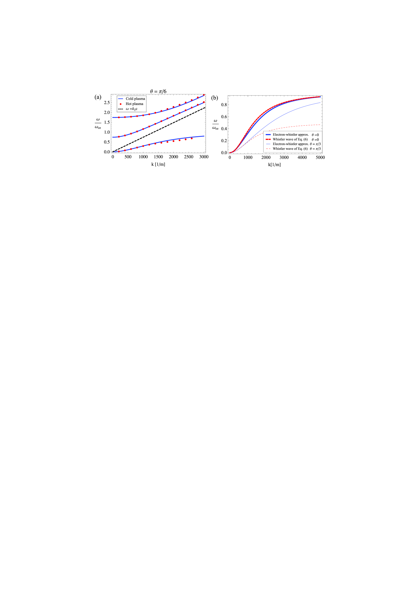
The whistler approximation is usually defined by ww
| (6) |
To show the whistler character of the lowest frequency solution of , we plot it together with the solution of Equation (6) as functions of for and , see Figure 1b. For there is very good agreement between the two solutions. For and wave numbers up to 1000 the two solutions overlap, but for higher wave numbers they deviate. This difference is due to the approximation used when deriving Equation (2), while when deriving the whistler wave dispersion given in Equation (6) in Reference ww no such approximation was used. By investigating the validity of the (5) dispersion we concluded that it yields valid results compared to the general dispersion relation for magnetic fields up to . In the following we will therefore limit our analysis to .
Including runaways, Equation (5) can be written as
| (7) |
where denotes the runaway contribution to the susceptibility tensor. The linear growth rate of a small perturbation of the wave frequency , is and is given by
| (8) |
where denotes the imaginary part and are the cold plasma dielectric tensor elements defined by Equation (4) evaluated at the unperturbed wave frequency: .
II.2 Magnetosonic-whistler
To evaluate the wave-particle interaction in the lower frequency region we analyze the dispersion relation in the frequency range . Interaction between these waves and strongly relativistic runaways has been studied before pokol ; fulop . However, in a near-critical field, it is more likely that the runaways are mildly relativistic, and as both the distribution function and the resonance condition is different, the analysis in previous work has to be generalized. In this frequency range the contributions to the dielectric tensor elements are
| (9) | |||
where and are the ion plasma and cyclotron frequencies, respectively. Substituting these into Equation (2) leads to the following dispersion relation
| (10) |
where is the Alfvén speed. In Reference fulop a simplified version of this dispersion relation
| (11) |
valid in the limit , was used to study destabilization of waves by an avalanching runaway electron distribution. The wave determined by Equation (10) can be identified as the generalized magnetosonic-whistler wave, as its simplified limit, Equation (11), for quasi-perpendicular propagation and
| (12) |
has been previously identified as the magnetosonic-whistler wave fulop .
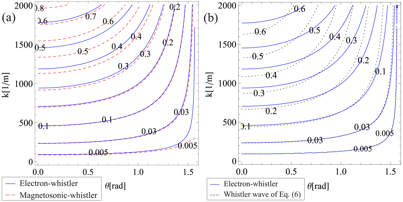
Figure 2 shows contour plots of the electron-whistler wave together with the magnetosonic-whistler wave (Figure 2a) and the electron-whistler wave together with the whistler approximation from Equation (6) (Figure 2b). The electron-whistler and magnetosonic-whistler waves approximately overlap with the whistler approximation for low (any propagation angle) and quasi-perpendicular propagation (any ). In the rest of the --space the electron-whistler and magnetosonic-whistler waves have different dispersion characteristics, as the magnetosonic-whistler approximation is not valid in the region of very high numbers because its frequency is assumed to be .
Including runaways, Equation (10) can be written as
and the linear growth rate of a perturbation of the wave frequency is
| (13) |
In the following section we will calculate the runaway contribution to the susceptibilities which will allow us to evaluate the linear growth rate of the wave.
III Runaway contribution
The susceptibility due to the runaway electron population is given by stix :
| (14) |
where
is the relativistic cyclotron frequency of the electrons, is the Bessel function of the first kind, , , is the normalized relativistic momentum, is the relativistic factor, is the normalized runaway distribution and is the order of resonance. The general (and implicit) condition for the resonant momentum is
| (15) |
If the distribution function is known, the resonance condition allows the integral in (14) to be evaluated using the Landau prescription.
III.1 Distribution of the runaway electrons
To calculate the runaway susceptibilities, the runaway distribution given in Equation (83) of Reference sandquist is used for the near-critical case
| (16) |
where
| (17) |
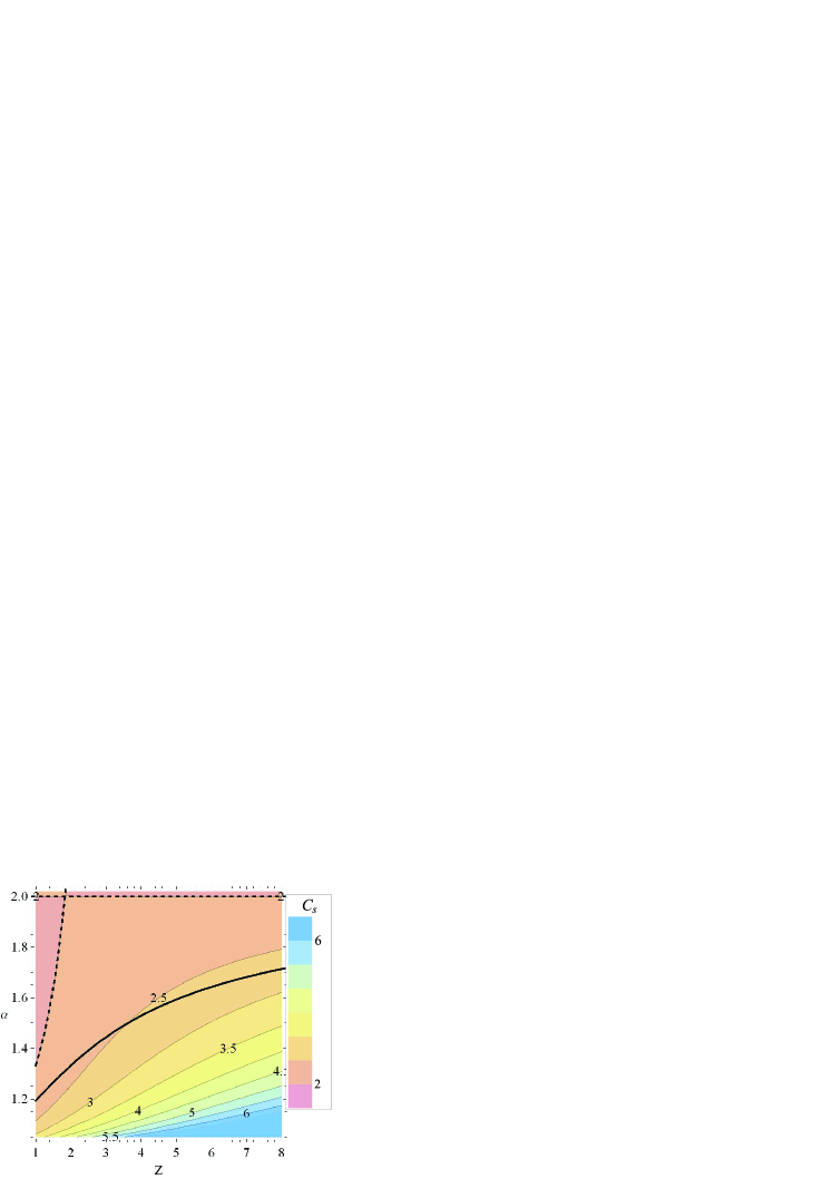
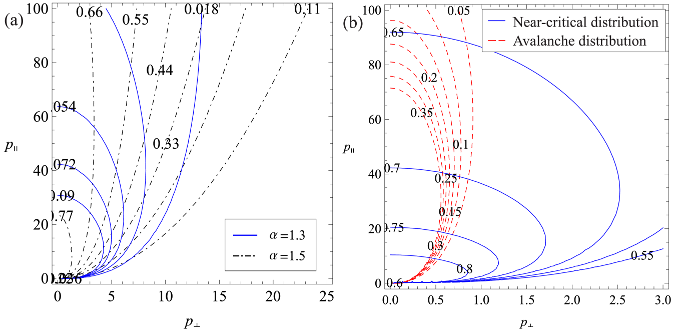
is the effective ion charge and is the confluent hypergeometric (Kummer) function. The distribution function given above was obtained by matching asymptotic expansions in five separate regions in momentum space. The calculation is similar to the one presented by Connor and Hastie connorhastie of runaway electron generation, but it is valid for near-critical electric field. Note, that to have a positive distribution function, the first argument of should be positive, leading to the condition . Furthermore, the condition as requires that . This gives a region in the - space where Equation (16) is valid. The parameter as function of and is plotted on Figure 3. The region between the solid and dashed lines gives the combinations of and for which the condition is fulfilled. This gives a restriction on the effective charge number, since if , the charge number can only be slightly more than unity. In tokamak plasmas seldom exceeds values of about . In the following we will only consider combinations of and such that . One such combination is and and this, together with the parameters , , are the baseline parameters of our study, and will be used in the rest of the paper unless otherwise is stated. Note, that although includes a term proportional to , its value varies very little in the parameter space where the distribution function is valid, as Figure 3 shows is between 2.5 and 3 in the region of interest, irrespective of the exact value of and . Therefore the distribution function is not very sensitive to these values.
Equation (16) is valid for all in the case of near-critical electric field. Note, that the integral of Equation (16) function in the whole momentum space is divergent. This is because the electric field continuously accelerates electrons and more and more electrons will run away. In spite of the continuous acceleration, the distribution is in quasi-steady state, as the water leaking out of an unplugged bath tub helander . However, as the existence of the electric field is finite in time, there is a maximum number of runaways and there is a maximum energy which runaway electrons can reach in reality. In the expressions for the runaway susceptibilities we use a normalized distribution function . The normalization constant in Equation (16) is obtained from
| (18) |
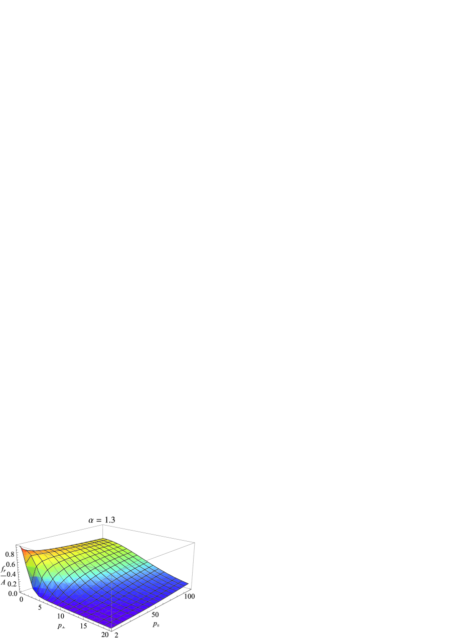
where is the normalized momentum corresponding to the maximum energy. This integral can be easily solved numerically if is known. The value of depends on the exact value and time evolution of the accelerating field. In this paper we approximated the maximum energy as , corresponding to . A typical value of the perpendicular momentum can be determined from the runaway distribution function. In the case of , this is . This value corresponds to MeV. Figure 4 shows Equation (16) for and . For the baseline parameters of our study this corresponds to the electric field of , while the critical field is .
It is instructive to compare the distribution in Equation (16) with the distribution derived for the case of secondary runaway generation pokol ; fulop ; fulop1
| (19) |
where and . The avalanche distribution is based on the solution of the kinetic equation for relativistic electrons in the limit of using the Rosenbluth-Putvinski runaway growth rate rosput
as boundary condition. Here is the collision time for relativistic electrons. This means that the runaway density grows exponentially as , where is the seed produced by primary generation. Note that for the avalanching distribution , independent of the maximum momentum. The distribution (19) is valid if secondary generation of runaways is dominant, as expected to be the case in large tokamak disruptions. In contrast, the distribution (16) is valid when primary runaway production is the main source of the superthermal electron population.
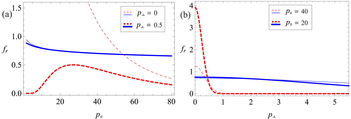
Comparing the two distributions, we note that the near-critical distribution function in Equation (16) represents a broader beam, with a less rapidly decaying tail. Figures 5-6 show the comparison between the near-critical and the avalanching distribution functions. Figure 5a shows the near-critical distribution for two different values of and . Figure 5b shows the comparison between the , case of the near-critical distribution with the avalanching distribution, which is significantly more beamlike. To illustrate that the distribution is more beamlike and more rapidly decaying in in the avalanche case, in Figure 6 we show the comparison between the near-critical and avalanching distributions for specific values of and . In spite of the differences noted above, the distribution functions in the and limits are similar in the sense that both have an anisotropy in the direction, and a smooth transition between the two can be envisioned based on Figure 5. The reason for using this particular distribution function (Eq. (16)) in the present work is that it is at the lower limit of that can possibly produce runaway electrons.
Although Equation (16) describes primary generation of runaways, it does not mean that the generation rate is small. Primary generation implies that the runaway generation is smaller than . But since is very large, primary generation can result in a substantial runaway electron population and its importance has been shown in many numerical simulations, see e.g. hakan .
III.2 Resonance condition
In a plasma with a slightly supercritical electric field, the characteristic value of the normalized momentum in the runaway region satisfies . To obtain an explicit formula for the resonant momentum, the expression should be substituted into the resonance condition, and that leads to
| (20) |
By using this general resonance condition, the expressions giving the imaginary parts of the runaway susceptibilities become quite complicated. The full expressions for the susceptibilities are given in Appendix A.
Only the resonant momenta are physically relevant. By studying the condition for different signs of , using the relation between and it can be shown that the Doppler resonances () cannot be satisfied for any of the solutions in Equation (5) or Equation (10).
Anomalous Doppler resonance
For the anomalous Doppler resonance () the condition, defining the physically relevant region of the resonant momentum, is
| (21) |
leading to , which is only satisfied for the electron-whistler branch and not for the other two solutions of Equation (5). Also the magnetosonic-whistler wave can be destabilized via this resonance.
Cherenkov resonance
For Cherenkov resonance (the case of ) the condition is
| (22) |
This also leads to the condition , narrowing down the possible waves once again to the electron-whistler wave and the magnetosonic-whistler wave. Summarizing the results above, we conclude that for , only the electron-whistler waves can yield physically relevant results out of the high frequency electron waves defined by the dispersion relation in Equation (5). The magnetosonic-whistler waves can also be destabilized via resonances. However, combining the region of the validity of the wave frequency with the resonance condition it can be seen that in the magnetosonic-whistler case the destabilization is most effective by very energetic (around ) runaway electrons.
IV Unstable waves
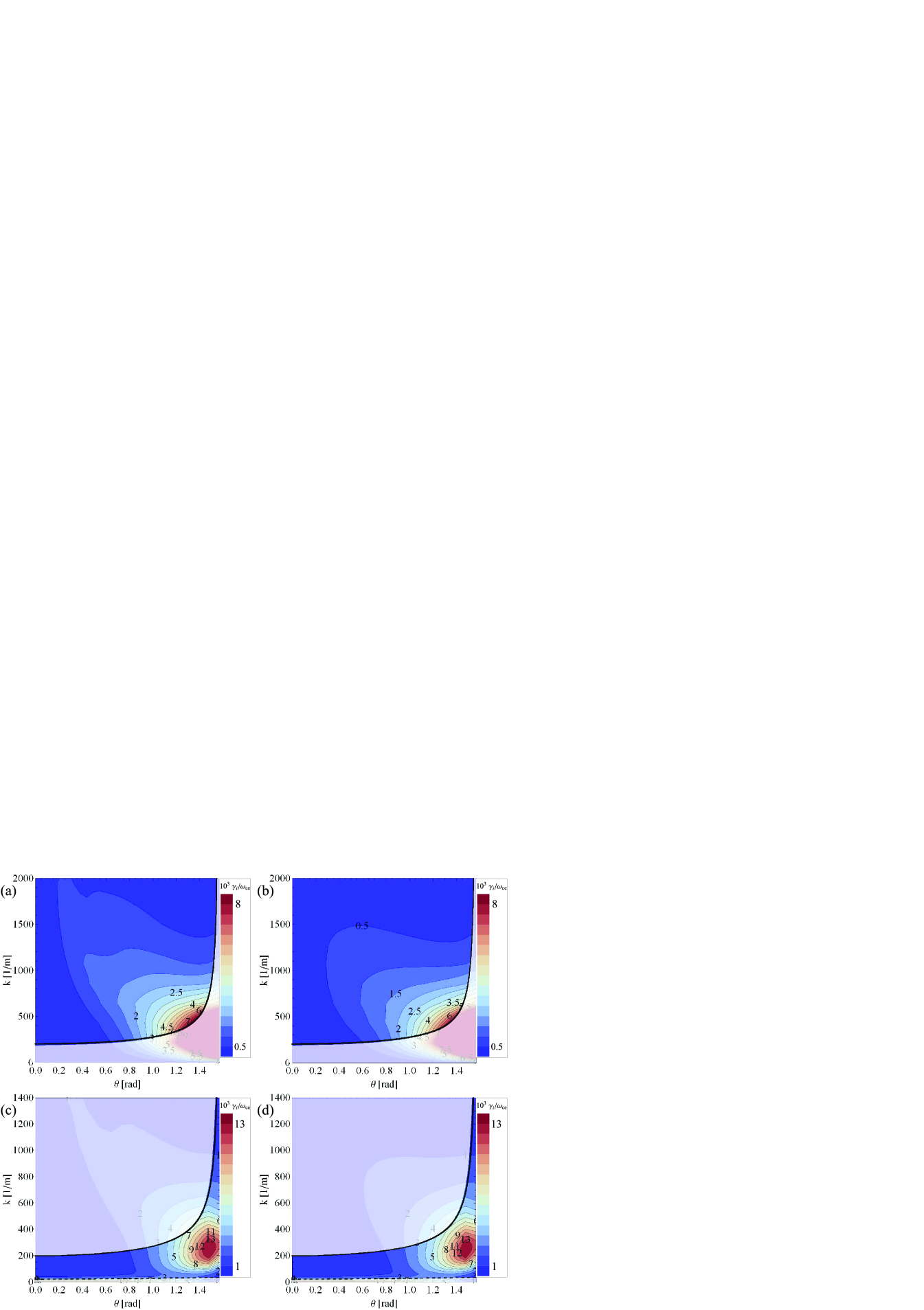
The instability growth rates for the electron-whistler and the magnetosonic-whistler waves can be calculated from Eqs. (8) and (13) as functions of k. Figure 7ab shows the growth rates for the electron-whistler wave using the ultrarelativistic limit and the general resonance condition, respectively, for the baseline parameters. The growth rate increases with decreasing throughout the range of validity of the electron-whistler approximation. Comparing Figure 7a and Figure 7b it can be seen that by using the ultrarelativistic condition one gets somewhat different results than by using the general condition, but the qualitative behaviour is the same.
Figure 7cd shows the growth rates for magnetosonic-whistler wave. In contrast to the electron-whistler wave, the growth rate has a well-defined maximum. However, as it was mentioned before, the resonance condition cannot be satisfied in the region close to the maximum growth rate unless the resonant energy is very high (around 10 MeV for the parameters given in the figure caption), which is only expected to be reached by few electrons in the near-critical case considered in this paper. Interestingly in both cases, the largest instability growth rate occurs for the region in the --space where the whistler approximation (6) is valid (see the low and perpendicular propagation part of Figure 2). However, we note that only high energy electrons can interact with the quasi-perpendicularly propagating whistler wave, therefore it is more likely that the electron-whistler branch with slightly higher and more oblique propagation is the one which is the most unstable wave.
IV.1 Most unstable wave
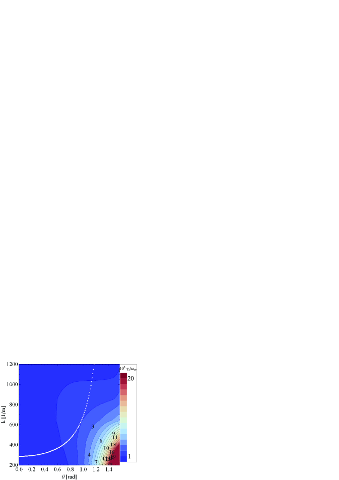
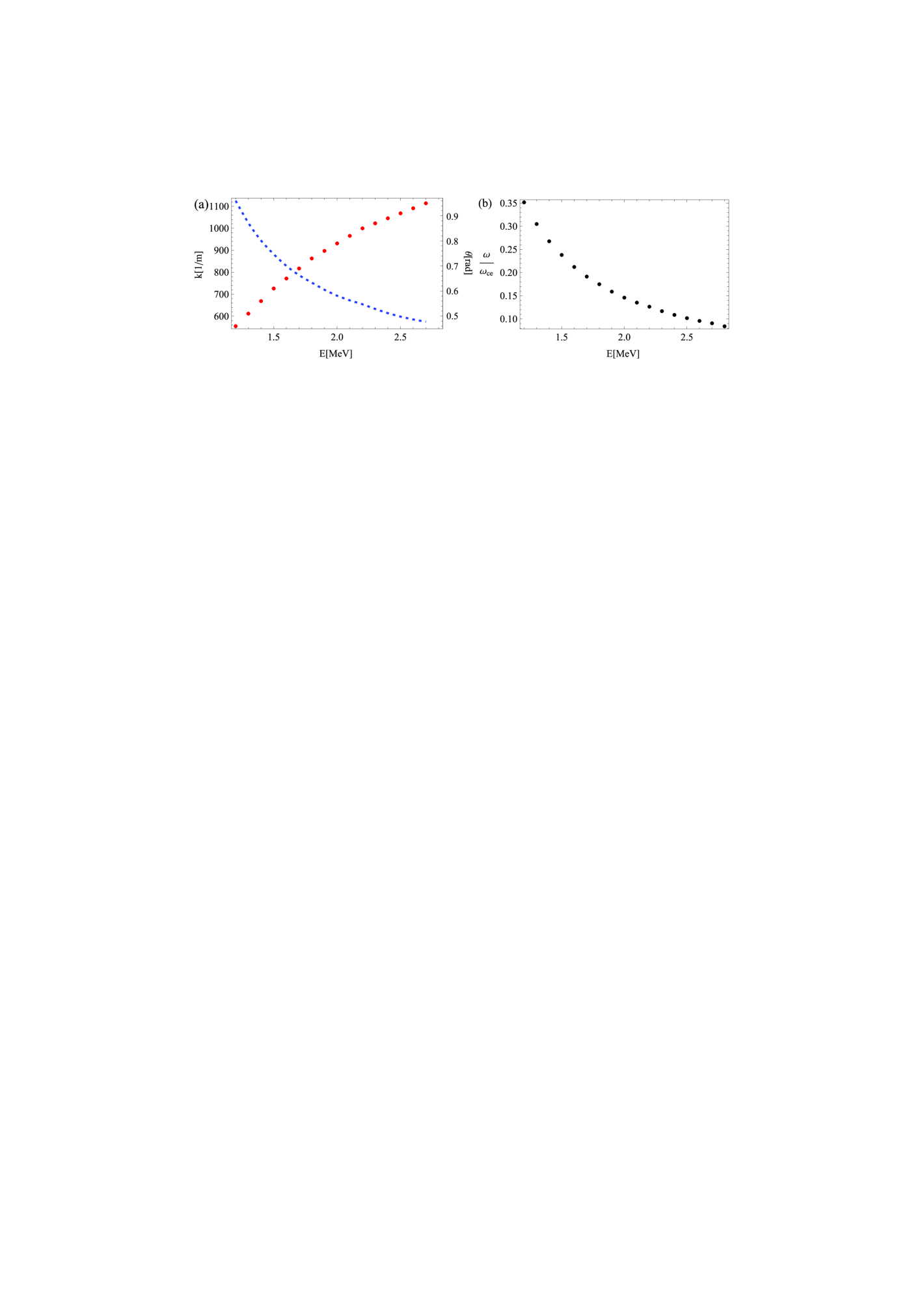
The normalized momentum corresponding to the maximum energy of MeV is approximately . The corresponding wave numbers and propagation angles of the electron-whistler wave can be calculated by using the general resonance condition and the dispersion relation. The growth rate and the values corresponding to are shown on Figure 8. The most unstable wave in the near-critical case is an electron-whistler wave with frequency (for a magnetic field of ), wave number of approximately , and angle of propagation .
It should be noted, that the parameters of the most unstable wave are sensitive to the magnetic field. The reason is that the resonance condition is highly dependent on the magnetic field through the gyrofrequency. Due to this fact, the condition for the momentum of the runaway electrons yields very different wave numbers for the most unstable wave. For example, if the magnetic field is T instead of the T on Figure 8, the resonant momentum yields wave number and . Therefore, by increasing the magnetic field, the wave number and frequency of the most unstable wave increase, while the angle of propagation decreases.
The wave number, propagation angle and frequency of the most unstable wave also depend on the maximum runaway energy. Figure 9 shows that as the energy grows the propagation angle becomes larger and the wave number and frequency drops. This means that for low energy runaway electrons (energies just above the critical energy for runaway acceleration) we expect frequencies slightly less than half of the electron cyclotron frequency, propagating angles of and wave numbers of 1000 . As the runaway energy grows the frequency and wave number of the most unstable wave falls.
IV.2 Stability diagram
In order to determine the stability limits, the instability growth rate of the wave has to be compared to the damping rates. In cold plasmas, collisional damping is dominant, and the damping is approximately equal to brambilla , where is the electron-ion collision time. In addition to collisional damping, the wave is damped due to the fact that the extent of the runaway beam is finite, and the wave energy is transported out of its region with a perpendicular group velocity. This mechanism can be accounted for by adding a convective damping term , where is the radius of the runaway beam fulop1 . The linear growth rate of a wave is thus , and the wave is unstable, if . A simple estimate of the order of magnitude of the damping rates shows that for typical parameters, and for reasonably narrow electron beams, the convective damping is expected to dominate if . However, as the plasma temperature seldom reaches such a high value in the relevant case of tokamak disruptions ward , collisional damping should not be neglected.
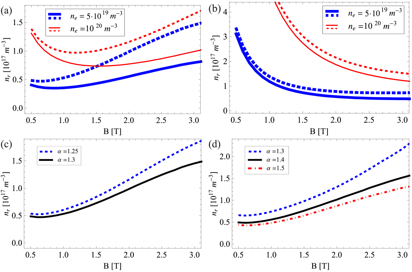
The linear stability threshold was determined in the following way. For any given value of the magnetic field the growth rate is calculated (for , , then adding them for all and ), then the collisional and convective damping rates are subtracted from it. The parameters of the most unstable wave are then determined. The stability threshold of the most unstable electron-whistler wave is shown on Figure 10a. We conclude that for typical parameters the runaway density needed to counter the damping rates, therefore to destabilize an electron-whistler wave is of the order of or . For the magnetosonic-whistler wave, the stability threshold is shown in Figure 10b. In this case we assumed , since in this case the resonant particles have higher energies than in the electron-whistler case. Figure 10cd shows the dependence of the stability threshold on the normalized electric field . We conclude that above , the runaway density needed for destabilization is sensitive to , for higher normalized electric field lower runaway density is needed to destabilize the wave. This dependence on is due to the fact that for a higher electric field the anisotropy of the runaway distribution and thus the destabilizing effect is stronger, therefore a lower density of runaways suffices for a resonant destabilization of the wave. This is by no means because of the special characteristics of the model distribution we used, but is due to the underlying physics.
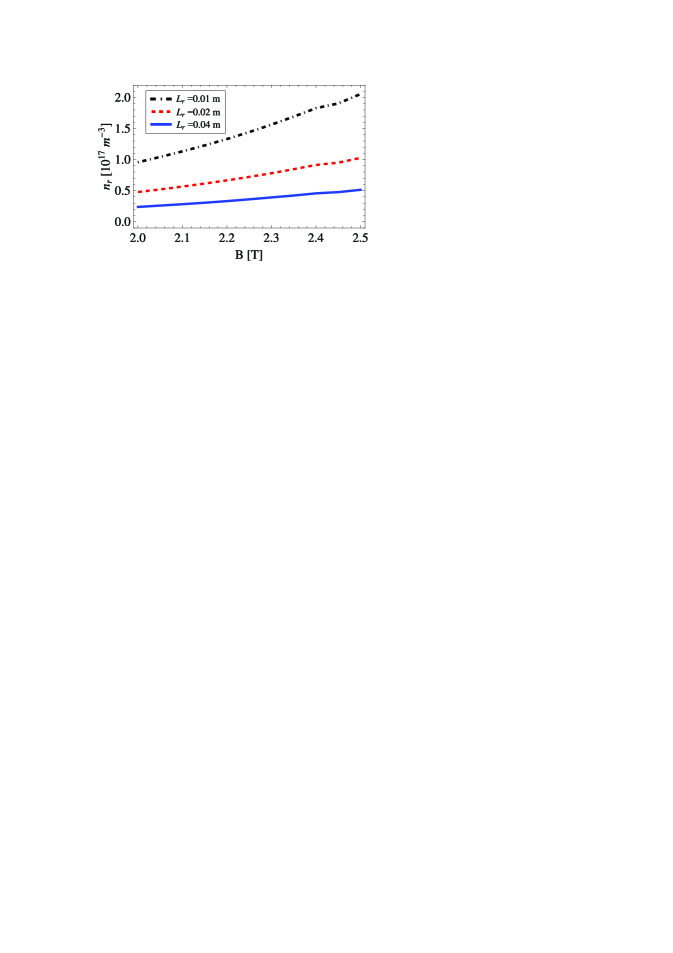
It is instructive to compare the order of magnitude of the runaway density required for destabilization of the whistler wave to the one that is measured in an experimental setup. Figure 11 shows the stability thresholds as function of magnetic field, for various runaway beam radii, for parameters relevant to an experiment in the T-10 tokamak savrukhin . We note that the runaway density needed for destabilization is about even for a narrow runaway beam. The runaway density estimated in the experiment was almost an order of magnitude higher than this: .
V Conclusions
The presence of high energy electrons is often associated with bursts of high-frequency waves. The emission of radiation is most often due to Bremsstrahlung and synchrotron radiation, but in certain cases they are due to instabilities caused by the anisotropy. The observation of these waves can help to determine the origin and evolution of the energetic electrons, and also in some cases, the properties of the background plasma ww . The instability may result in pitch-angle scattering induced isotropization and may therefore prevent the harmful effects of the runaway electron beam pokol .
The reason for the generation of an anisotropic runaway electron population is the high electric field that is often caused by reconnection events in magnetized plasmas. In previous calculations regarding waves driven by runaways the electric field was assumed to be much higher than the critical field . This is not often the case in reality. Therefore, in this paper we use an electron distribution function that is valid in the near-critical case. We show that in this case, the distribution is broader and less rapidly decaying compared to the case.
By studying the linear growth rate of the electron-whistler branch (valid in the frequency region ) and the magnetosonic-whistler branch (valid in the frequency region ) separately, we find that the frequency of the most unstable wave is in the region where these overlap and have characteristics similar to the whistler approximation. For typical tokamak parameters we find that the frequency of the most unstable wave is around , in the near-critical case with and . The frequency and wave number of the most unstable wave depends strongly on the magnetic field and on the maximum runaway energy. By comparing the ultra-relativistic limit of the resonance condition and the general one we show that although the behaviour of the instability growth rates of the electron-whistler and magnetosonic-whistler waves are similar, the actual values for the growth rate may differ, and therefore the frequency and wave number of the most unstable wave might be different.
The instability growth rate of the electron-whistler wave was compared to the collisional and convective damping rates. We find that the number density of runaways that is required to destabilize the waves increases with increasing magnetic field. For low magnetic fields the convective damping decreases, while the collisional damping rate remains constant, making it dominant in this region. As the growth rate also decreases, the stability limit is high for low magnetic fields. We investigated the stability of the whistler waves for parameters relevant to the T-10 tokamak savrukhin , where the effective electric field is near-critical. We found that the observed runaway density is about an order of magnitude higher than the density needed for the most unstable electron-whistler wave to be destabilized. Thus the runaway population may indeed give rise to this whistler wave.
The importance of this study is that it considers the case where the electric field is near critical, which is opposite to the other limit that has been considered in previous work pokol ; fulop ; fulop1 (when the electric field is far above the critical). By investigating this case, we show that the high-frequency instabilities are qualitatively similar, but have different frequencies and wave numbers. This result may open up the possibility of diagnostics. Understanding the properties of the waves destabilized by runaway electrons can be important in view of obtaining information about the energetic electron population and the background plasma. Regardless of the fact that the distribution used in this work is only valid in the near-critical case, if we compare it to the avalanche distribution we observe a smooth transition between the two, and so we expect that the distribution does not change qualitatively. Also, the characteristics of the growth rates in the near-critical and high electric field limits are similar, in the sense that the maximum of the growth rate is at low wave numbers and near-perpendicular propagation in both cases fulop . The differences in the parameters of the most unstable wave for near-critical and avalanching cases are mainly due to the maximum runaway energy. The similarity of the results, added to the relaxation of the approximations used in previous work, opens the way toward more general numerical studies of wave-particle interaction for arbitrary electric fields.
The whistler waves, if they grow to significant amplitude, in principle could perturb the background magnetic field and lead to efficient transport of particles (specially energetic ones) out from the plasma. The effect of magnetic field perturbation has been studied before radialdiffusion ; papp1 ; papp2 , and it has been shown that runaway avalanches can be prevented altogether with sufficiently strong radial diffusion. However, the magnetic fluctuation level that is required for this to happen is estimated to be and the magnetic fluctuation level induced by these high-frequency whistler waves would be several orders of magnitude lower than this value. Therefore, as mentioned before, the runaway electron population will be affected mostly through pitch-angle scattering and concomitant isotropization and synchrotron radiation damping.
Acknowledgements
This work, supported by the European Communities under the contract of association between EURATOM, Vetenskapsrådet and the Hungarian Academy of Sciences, was carried out within the framework of the European Fusion Development Agreement. The authors are grateful to H. Smith, G. Papp and P. Helander for fruitful discussions. One of the authors acknowledges the financial support from the FUSENET Association. The views and opinions expressed herein do not necessarily reflect those of the European Commission.
Appendix A: Runaway susceptibilities
In the general case the susceptibilities have the following form:
where we used the resonance condition to replace the factor . The and terms only differ in multiplicative constants and will be presented later.
For a general function we can rewrite the integral in as follows
| (25) |
where , , , and . Changing variables so that
Equation (25) yields
| (26) | |||
Using the above expression to solve the integrals in the runaway susceptibilities, we arrive to the following formulas:
where
Similarly the other two terms of the runaway susceptibility:
Equation (Appendix A: Runaway susceptibilities) gives the real part of the runaway susceptibility since this term is the one needed in the expression for the growth rate. By substituting these runaway susceptibilities into the expression of the growth rate, the calculations yield results in the general, relativistic case regarding the runaway electrons interacting with the corresponding wave.
References
- (1) J.A. Wesson, R.D. Gill, M. Hugon, F.C. Schüller, J.A. Snipes, D.J. Ward, D.V. Bartlett, D.J. Campbell, P.A. Duperrex, A.W. Edwards, R.S. Granetz. N.A.O. Gottardi, T.C. Hender, E. Lazzaro, P.J. Lomas, N. Lopes Cardozo, K.F. Mast, M.F.F. Nave, N.A. Salmon, P. Smeulders, P.R. Thomas, B.J.D. Tubbing, M.F. Turner and A. Weller, Nucl. Fusion 29, 641 (1989).
- (2) M. Tavani, M. Marisaldi, C. Labanti, F. Fuschino, A. Argan, A. Trois, P. Giommi, S. Colafrancesco, C. Pittori, F. Palma, M. Trifoglio, F. Gianotti, A. Bulgarelli, V. Vittorini, F. Verrecchia, L. Salotti, G. Barbiellini, P. Caraveo, P. W. Cattaneo, A. Chen, T. Contessi, E. Costa, F. D’Ammando, E. Del Monte, G. De Paris, G. Di Cocco, G. Di Persio, I. Donnarumma, Y. Evangelista, M. Feroci, A. Ferrari, M. Galli, A. Giuliani, M. Giusti, I. Lapshov, F. Lazzarotto, P. Lipari, F. Longo, S. Mereghetti, E. Morelli, E. Moretti, A. Morselli, L. Pacciani, A. Pellizzoni, F. Perotti, G. Piano, P. Picozza, M. Pilia, G. Pucella, M. Prest, M. Rapisarda, A. Rappoldi, E. Rossi, A. Rubini, S. Sabatini, E. Scalise, P. Soffitta, E. Striani, E. Vallazza, S. Vercellone, A. Zambra and D. Zanello, Phys. Rev. Lett. 106, 018501 (2011).
- (3) E. Moghaddam-Taaheri and C.K. Goertz, Astrophys. J. 352, 361 (1990).
- (4) G. Pokol, T. Fülöp and M. Lisak, Plasma Phys. Control. Fusion 50, 045003 (2008).
- (5) T. Fülöp, G. Pokol, P. Helander and M. Lisak, Phys. Plasmas 13, 062506 (2006).
- (6) T. Fülöp, H.M. Smith and G. Pokol, Phys. Plasmas 16, 022502 (2009).
- (7) R.D. Gill, B. Alper, M. de Baar, T.C. Hender, M.F. Johnson, V. Riccardo and contributors to the EFDA-JET Workprogramme, Nucl. Fusion 42, 1039 (2002).
- (8) R. Yoshino, S. Tokuda and Y. Kawano, Nucl. Fusion 39, 151 (1999).
- (9) P.V. Savrukhin, Phys. Rev. Lett. 86, 14 (2001).
- (10) J. Riemann, H.M. Smith and P. Helander, Phys. Plasmas 19, 012507 (2012).
- (11) P Sandquist, S.E. Sharapov, P. Helander and M. Lisak, Phys. Plasmas 13 072108 (2006).
- (12) T. H. Stix, Waves in plasmas, American Institute of Physics, New York, 1992.
- (13) S. Sazhin, Whistler-mode waves in a hot plasma, Cambridge University Press, Cambridge, 1993.
- (14) W. Connor and R.J. Hastie, Nucl. Fusion 15, 415 (1975).
- (15) P. Helander, L.-G. Eriksson and F. Andersson, Plasma Phys. Control. Fusion 44, B247 (2002).
- (16) M.N. Rosenbluth and S.V. Putvinski, Nucl. Fusion 37, 1355 (1997).
- (17) H.M. Smith, P. Helander, L.-G. Eriksson, D. Anderson, M. Lisak and F. Andersson, Phys. Plasmas 13 102502 (2006).
- (18) M. Brambilla, Phys. Plasmas 2, 1094 (1995).
- (19) D.J. Ward and J.A. Wesson, Nucl. Fusion 32 1117 (1992).
- (20) P. Helander, L.-G. Eriksson and F. Andersson, Phys. Plasmas 7, 4106 (2000).
- (21) G. Papp, M. Drevlak, T. Fülöp, P. Helander and G.I. Pokol, Plasma Phys. Control. Fusion 53, 095004 (2011).
- (22) G. Papp, M. Drevlak, T. Fülöp and P. Helander, Nucl. Fusion 51 043004 (2011).