Electron spin resonance spectroscopy of small ensemble paramagnetic spins using a single nitrogen-vacancy center in diamond
Abstract
A nitrogen-vacancy (NV) center in diamond is a promising sensor for nanoscale magnetic sensing. Here we report electron spin resonance (ESR) spectroscopy using a single NV center in diamond. First, using a 230 GHz ESR spectrometer, we performed ensemble ESR of a type-Ib sample crystal and identified a substitutional single nitrogen impurity as a major paramagnetic center in the sample crystal. Then, we carried out free-induction decay and spin echo measurements of the single NV center to study static and dynamic properties of nanoscale bath spins surrounding the NV center. We also measured ESR spectrum of the bath spins using double electron-electron resonance spectroscopy with the single NV center. The spectrum analysis of the NV-based ESR measurement identified that the detected spins are the nitrogen impurity spins. The experiment was also performed with several other single NV centers in the diamond sample and demonstrated that the properties of the bath spins are unique to the NV centers indicating the probe of spins in the microscopic volume using NV-based ESR. Finally, we discussed the number of spins detected by the NV-based ESR spectroscopy. By comparing the experimental result with simulation, we estimated the number of the detected spins to be 50 spins.
I introduction
A nitrogen-vacancy (NV) center is a paramagnetic defect center in diamond. A NV center is a great testbed to investigate quantum physics because of its unique electronic, spin, and optical properties including its stable fluorescence (FL) signals, Gruber et al. (1997) long decoherence time, Kennedy et al. (2003); Gaebel et al. (2006); Childress et al. (2006); Balasubramanian et al. (2009); Takahashi et al. (2008) and capability to initialize the spin states of NV centers by applying optical excitation and to readout the states by measuring the FL intensity. Jelezko et al. (2004) A NV center is also a promising magnetic sensor Degen (2008); Balasubramanian et al. (2008); Maze et al. (2008); Taylor et al. (2008); Steinert et al. (2013); Kaufmann et al. (2013); Mamin et al. (2013); Staudacher et al. (2013); Ohashi et al. (2013); Müller et al. (2014); Maletinsky et al. (2012) because its extreme sensitivity to the surrounding electron Gaebel et al. (2006); Hanson, Gywat, and Awschalom (2006); Hanson et al. (2008) and nuclear spins. Childress et al. (2006); Balasubramanian et al. (2009) Spin sensitivity of electron spin resonance (ESR) spectroscopy is drastically improved using NV centers. ESR spectrum of small ensemble electron spins has been measured using a double electron-electron resonance (DEER) spectroscopy with single NV centers. de Lange et al. (2012); Mamin, Sherwood, and Rugar (2012); Laraoui, Hodges, and Meriles (2012); Knowles, Kara, and Atatüre (2014) ESR detection of a single electron spin has also been demonstrated using the DEER technique. Grinolds et al. (2013); Sushkov et al. (2014); Shi et al. (2015) In addition, bio-compatibility and excellent chemical/mechanical stability of diamond makes a NV center suitable for applications of nanoscale magnetic sensing and magnetic resonance spectroscopy in biological systems. Hall et al. (2000); McGuinness et al. (2011); Le Sage et al. (2013); Shi et al. (2015)
In this article, we discuss ESR spectroscopy of a small ensemble of electron spins using single NV centers in diamond. Although the state-of-the-art of NV-based ESR spectroscopy is the detection of a single electron spin, the small ensemble measurement is often advantageous for applications of NV-based ESR because of less sophisticated sample preparation (e.g. higher density of the target spins which increases the coupling to the NV) and more sensitive detection (e.g. more pronounced changes in the coherence () and population () decays), and still enables to probe nanoscale local environments which may be different from the bulk properties. On the other hand, it is challenging to estimate the detected number of spins from the small ensemble measurement.
In the investigation, our experiment is performed with a type-Ib diamond crystal at room temperature. Using a 230 GHz ESR spectrometer, we first perform ensemble ESR of the sample crystal and find that a major paramagnetic impurity in the sample crystal is a substitutional single nitrogen center (N spin; also known as P1 center). Next, we detect a single NV center using FL autocorrelation and optically detected magnetic resonance (ODMR) measurements. We then carry out Rabi, free-induction decay (FID) and spin echo (SE) measurements of the single NV center to study static and dynamic properties of bath spins surrounding the NV center. We also employ DEER spectroscopy to measure ESR signals of the bath spins using the NV center. The detected bath spins are identified as N spins from the analysis of the observed ESR spectrum. Based on the intensity of the observed NV-based ESR signal, the detected magnetic field by the DEER measurement is 6 T (equivalent to the magnetic field caused by a single spin with the distance of 7 nm). We also study several single NV centers in the same crystal and find heterogeneity in their spin properties which indicates that our ensemble measurement still proves bath spins in the microscopic scale. Finally, we introduce a computational simulation method for the estimate of the number of the detected spins. By comparing the experimental result with simulation, we estimate the number of the detected spins to be 50 spins.
II results and discussion
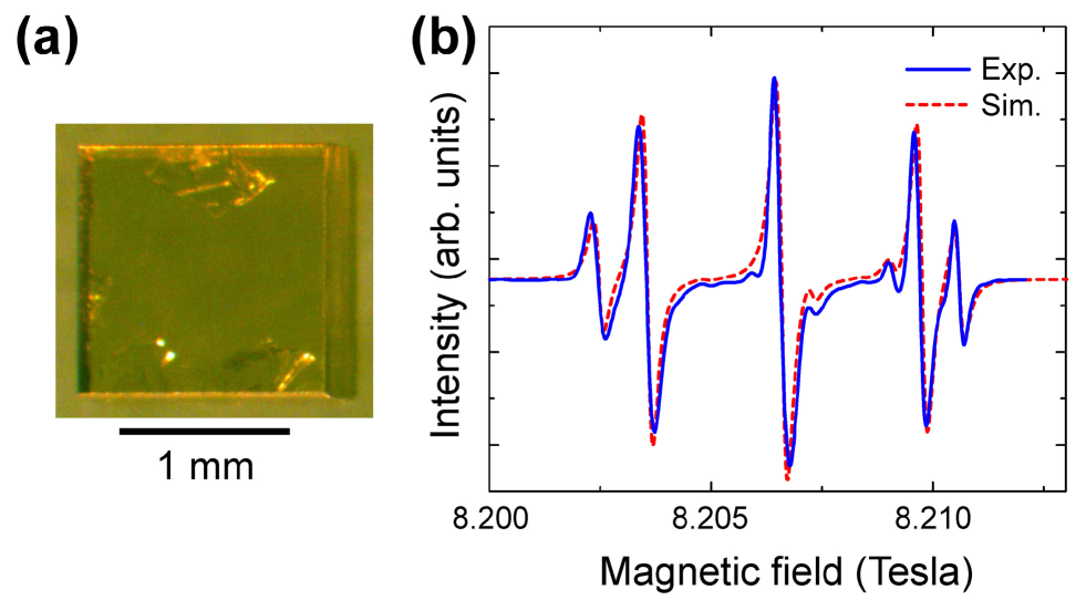
We studied a single crystal of high-temperature high-pressure type-Ib diamond, which is commercially available from Sumitomo electric industries. The size of the diamond crystal is mm3 (see Fig. 1(a) inset). The concentration of N spins is 10 to 100 ppm, corresponding to to N spins existing in diamond. First, using a 230 GHz ESR spectrometer, Cho, Stepanov, and Takahashi (2014) we measured ensemble ESR of the sample diamond crystal at room temperature to characterize its bulk properties where the magnetic field was applied along the 111-direction of the single crystal diamond in the measurement. As shown in Fig. 1(b), continuous-wave (cw) ESR spectroscopy revealed five-line ESR signals corresponding to the N spins. The ESR intensity of the N spins was drastically stronger than the remaining signals, which indicates that the number of N spins dominates the spin population in the sample. Moreover, no ESR signals from NV centers and other paramagnetic impurities were observed in the ESR measurement because of their low concentration in the sample crystal. The spin Hamiltonian of N spin is given by
| (1) |
where is the Bohr magneton, is the external magnetic field, and are the -values of the N electron spin, and and are the electronic and nuclear spin operators, respectively. is the anisotropic hyperfine coupling tensor to nuclear spin. The gyromagnetic ratio of nuclear spin () is 3.077 MHz where is the Planck constant. The last term of the Hamiltonian is the nuclear quadrupole couplings. The previous studies measured , , MHz, MHz and MHz. Loubser and Vanwyk (1978); Smith et al. (1959); Takahashi et al. (2008) As shown in Fig. 1(b), the experimental data agree well with simulated ESR spectrum using Eq. (1) and the previously determined parameters.
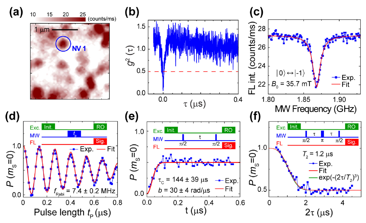
Figure 2 shows ODMR measurements of a single NV center in the diamond crystal. The ODMR experiment was performed using a home-built confocal microscope system. Abeywardana et al. (2014) For microwave excitations, two microwave synthesizers, a power combiner, and a 10 watt amplifier were connected to a 20 m-thin gold wire placed on a surface of the diamond sample. First a FL image of the diamond was recorded in order to map out FL signals in the diamond crystal (see Fig. 2(a)). After choosing an isolated FL spot, we carried out the autocorrelation and cw ODMR measurements in order to identify FL signals from a single NV center. As shown in Fig. 2(b), the autocorrelation measurement of the chosen FL spot revealed the dip at zero delay which confirmed the FL signals originated from a single quantum emitter. In addition, cw ODMR measurement of the selected single NV center was performed with application of the external magnetic field () of 35.7 mT along the 111 axis. As shown in Fig. 2(c), the reduction of the FL intensity was observed at the microwave frequency of 1.868 GHz corresponding to the ODMR signal of the transition of the NV center. Thus, the observations of the autocorrelation and cw ODMR signals confirmed the successful identification of the single NV center (denoted as NV 1).
Next, we performed pulsed ODMR measurements of NV 1. In the pulsed measurements, a NV center was first prepared in the state by applying an initialization laser pulse, and the microwave pulse sequence was applied for the desired manipulation of the spin state of the NV center, then the final spin state was determined by applying a read-out laser pulse and measuring the FL intensity. In addition, the FL signal intensity was mapped into the population of the NV’s state () using two references (the maximum and minimum FL intensities corresponding to the and states, respectively). de Lange et al. (2010) Moreover, the pulse sequence was averaged on the order of - times to obtain a single data point. First, the Rabi oscillation measurement was performed at mT and 1.868 GHz, which corresponds to the transition of NV 1. As the microwave pulse length () was varied in the measurement, pronounced oscillations of was observed as shown in Fig. 2(c). By fitting the observed Rabi oscillations to the sinusoidal function with the Gaussian decay envelope, Hanson et al. (2008) the lengths of - and -pulses for NV 1 were determined to be 34 and 68 ns, respectively. Second, FID was measured using the Ramsey fringes. The pulse sequence are shown in the inset of Fig. 2(e). As seen in Fig. 2(e), the FL intensity of NV 1 was recorded as a function of free evolution time () and FID was observed in the range of ns. Third, we carried out the SE measurement. Figure 2(f) shows the FL intensity as a function of free evolution time (2). As shown in the inset of Fig. 2(f), the applied microwave pulse sequence consists of the conventional spin echo sequence, widely used in ESR spectroscopy, Schweiger and Jeschke (2001) and an additional -pulse at the end of the sequence to convert the resultant coherence of a NV center into the population of the state.Jelezko et al. (2004) The FID and SE decay in electron spin baths have been successfully described by treating the bath as a classical noise field () where was modeled by the Ornstein-Uhlenbeck (O-U) process with the correlation function , where the spin-bath coupling constant () and the rate of the spin flip-flop process between the bath spins (). Klauder and Anderson (1962); Hanson et al. (2008) The FID and SE decay due to the O-U process are given by,
| (2) |
and
| (3) |
where = 2.3 MHz is the hyperfine coupling of NV center. Loubser and Vanwyk (1978) In the quasi-static limit () indicating slow bath dynamics, where is the spin decoherence time. Klauder and Anderson (1962); Hanson et al. (2008); Wang and Takahashi (2013) By fitting both FID and SE data (Fig. 2(e) and (f)) simultaneously with Eqs.(2) and (3), we obtained and to be 30 4 (rad/) and 144 39 s, respectively. The result indicates that the surrounding spin bath is in the quasistatic limit (), therefore, () of NV 1 is 1.2 s. Using the previous study, Wang and Takahashi (2013) the local concentration of the bath spins around NV 1 is estimated to be 20 ppm.
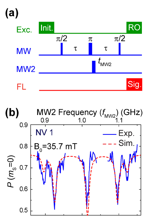
Furthermore, we performed NV-based ESR using DEER spectroscopy at mT (1.868 GHz corresponding to the transition). Figure 3(a) shows the pulse sequence used in the DEER measurements,de Lange et al. (2012); Mamin, Sherwood, and Rugar (2012); Laraoui, Hodges, and Meriles (2012) which was adopted from the field of ESR. Schweiger and Jeschke (2001) The DEER sequence consists of the spin echo sequence for a NV center and an additional -pulse at different microwave frequency (denoted as MW2 in Fig. 3(a)). When the additional -pulse is resonant with surrounding electron spins near the NV center, the magnetic moments of the surrounding spins are flipped, and this alters the magnetic dipole field experienced by the NV center from the surrounding spins during the second half of the spin echo sequence. The alteration causes a shift in the Larmor frequency of the NV center, which leads to different phase accumulation of the Larmor precession during the second half of the sequence from the first half. As a result, the NV center suffers phase-shift in the echo signal and reduction of FL intensity from the original spin echo signal is observed. As shown in Fig. 3(b), we monitored the spin echo intensity of NV 1 at a fixed as a function of , and observed clear intensity reductions at five frequencies ( 0.90, 0.92, 1.01, 1.10, and 1.12 GHz). In the measurement, ns and ns were chosen to maximize the NV-based ESR signals. As shown in Fig. 3(b), the resonant frequencies of the observed NV-based ESR signals were in a good agreement with the ESR of N spins calculated from Eq. (1), which confirms the observation of N spin ESR spectrum. The DEER intensity () represents the change of the SE intensity given by the change in the effective dipolar field (). Assuming that -flip of the N spins is instantaneous (i.e. the effect of a finite width of the pulse was not considered), = where is the -value of the NV center, Loubser and Vanwyk (1978) is the reduced Planck constant, and ns in the present case. In addition, including the effects of decay, the NV-based ESR signal in is given by,
| (4) |
Using Eq. (4), we obtained that the intensity of the NV-based ESR at GHz () corresponds to 6 T. This magnetic field is equivalent to the dipole magnetic field from a single spin with the NV-spin distance () of 7 nm ( with , , = 2 and = 1/2).
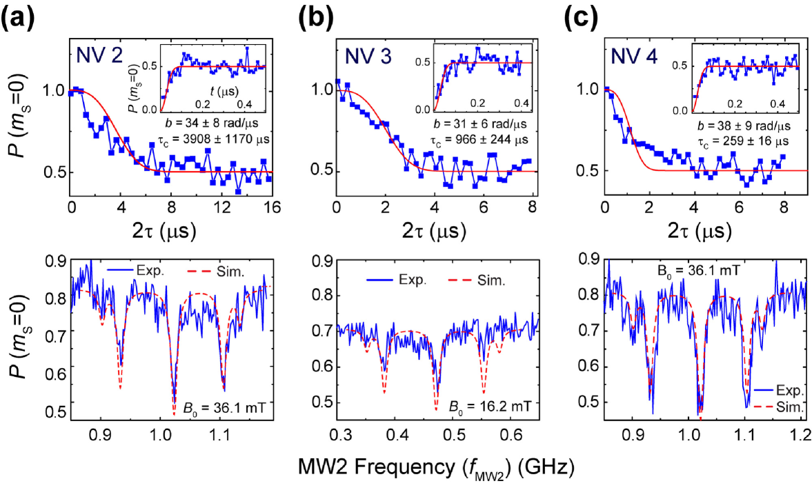
In addition to the investigation of NV 1, we have studies other NVs in the same diamond crystal. Figure 4 shows the set of FID, SE and DEER data from other three NV centers (labeled as NV 2-4). The results from NV 1-4 were different because of their heterogeneous nanoscale local environments. As shown in Fig. 4(a)-(c), we found that the obtained values were varied widely from 144 s to 3908 s. On the other hand, the variation of = 30-38 rad/ is much smaller than . As the result, of NV 1-4 ranges from 1.2 to 3.4 s. We also noticed that all NV 1-4 are in the quasistatic limit (). As shown in Fig. 3(b) and Fig. 4, the NV-based ESR spectra of NV 1-4 were also quite different. The NV-based ESR spectra from NV 1, 2 and 4 displays five-line ESR signals (Fig. 3(b) and Fig. 4(a)(c)) whereas NV 3 only shows three visible signals at 0.381 0.474 and 0.553 GHz (Fig. 4(b)). Possible reasons of the difference are heterogeneity of the number and the spatial configuration of N spins around the NV centers, and an uneven distribution of the N spin orientations due to a small number of N bath spins.
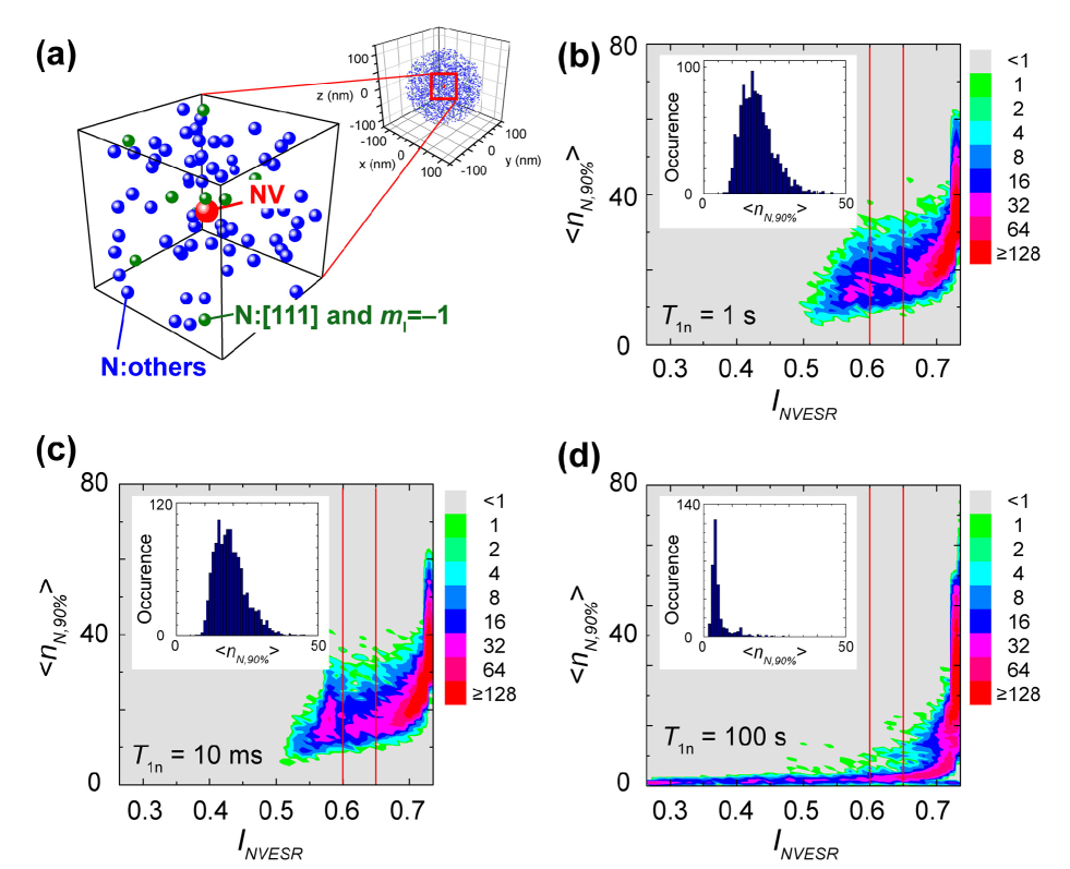
Finally, we analyze the intensity of the observed NV-based ESR signal to estimate the number of the detected N spins. Our analysis here focuses on the signal at GHz corresponds to the transition of N spins oriented along the 111 direction (Fig. 3(b)). In the analysis, we simulate DEER intensities by calculating the effective magnetic dipole field at the NV center from the surrounding N spins (). First step of the simulation was to generate a model configuration of the NV center and N spins in a diamond lattice, and this was done by placing the NV center at the origin of the diamond lattice and assigning the positions of N spins randomly in the lattice sites (see Fig. 5(a)). Based on the measurement ( = 1.2 s 20 ppm), 18,000 N spins were placed in the simulated diamond lattice with a diameter of 200 nm. Next, we randomly chose the orientation of N spins where only a quarter of N spins were assigned along the 111 direction and the rest of N spins were assigned along the other three directions, i.e., , , and . We then assigned the nuclear spin value () of either , , or to all N spins with equal probability. For the simulation, we only considered the contribution coming from the N spins oriented along the 111 direction with (The signal at GHz in Fig. 3(b)). Thus, was computed from only -th of all N spins in the simulated lattice on average (1500 N spins). Finally we assigned the electron spin value () of either or with equal probability to the N spins.
is given by the sum of individual dipolar field from each N spin as,
| (5) |
where is the dipolar field strength of -th N spin at the NV center, is the number of the N spins oriented along the 111 direction with , is the vacuum permeability, and are the magnitude and polar angle of the vector that connects the NV center and -th N spin, respectively, and is the electron spin value of -th N spin. The mutual flip-flops within N electron spins was also not considered because of a low rate of the spin flip-flop process during the measurement, i.e. (see Fig. 2(e)). We then calculated the number of N spins () out of to obtain more than 90 of the by successively adding individual dipolar field term from each N spin in descending order of magnitude (i.e., when ). In addition, we took into account for the electron and nuclear spin relaxations of N spins during the DEER measurement time ( s with averaging) by statistically re-assigning the electron and nuclear spin values ( and ) according to the electron and nuclear longitudinal relaxation times ( and ), respectively. Although has been investigated previously (10 ms),Reynhardt, High, and Vanwyk (1998); Takahashi et al. (2008) has not been reported before to the best of our knowledge. In the simulation, we used ms and considered to be 10 ms, 1 s and 100 s, therefore the assignment of happens times for s ( and 1 times for ms and 100 s, respectively) and a total of iterations (100 s/) occurs during the simulation. Then, what we finally computed were the average of values of and (i.e., and ), therefore, by rewriting Eq. (4), the simulated NV-based ESR signal is given by,
| (6) |
In addition, in order to see the spatial configuration dependence on and , we repeated the procedure described above for spatial configurations and calculated values of and .
Figure 5(b)-(d) shows the simulated result of as a function of (Eq. (6)) for s, 10 ms, and 100 s, respectively, from spatial configurations. As shown in Fig. 5(b), the number of the N spins that contribute to the NV-based ESR signal () depends on the detected . We first noted that, for all configurations we simulated, only a small portion (60) out of 1500 N spins contributes to more than 90 of on average. In the case of homogeneously distributed N spins, the 60 spins are located in a sphere with 70 nm diameter. Moreover, when the NV-based ESR intensity is large (), is smaller because in such spatial configurations is only dominated by a smaller ensemble of the N spin located in the vicinity of the NV center. In addition, there was little observation of (i.e., because a small probability exists for the NV center to be coupled with a single or a few N spins with the 20 ppm N concentration and the resultant is a weighted sum of many oscillatory functions with different frequencies. On the other hand, when the NV-based ESR intensity is small () (i.e. 0.73), is larger because the N spins in such spatial configurations spread uniformly and the N spins located farther away from the NV also contribute to . The experimentally observed NV-based ESR intensity was (see Fig. 3(b)). The inset of Fig. 5(b) shows a histogram of the occurrence of from the simulation that yielded -0.65. The occurrence was in the range of for s. Moreover, as shown in Fig. 5(c), with ms was similar to the result with s (The occurrence was in the range of ). On the other hand, in the case of s, the distribution was slightly different and the occurrence was in as shown in Fig. 5(d). Thus, from the simulation, the number of N spins in the present NV-based ESR measurement is estimated to be 50 spins.
III Summary
In summary, we presented ESR spectroscopy using a single NV center in diamond. First, we demonstrated the identification of microscopic spin baths surrounding a single NV center and the investigation of static and dynamic properties of the bath spins using Rabi, FID, SE measurements as well as NV-based ESR spectroscopy. We also performed the investigation with several other single NV centers in the diamond sample and found that the properties of the bath spins are unique to the NV centers. Finally, by analyzing the intensity of the NV-based ESR signal using the computer simulation, we estimated the detected spins in the DEER measurement to be 50 spins.
IV Acknowledgements
This work was supported by the National Science Foundation (DMR-1508661), the USC Anton B. Burg Foundation and the Searle scholars program (S.T.).
References
- Gruber et al. (1997) A. Gruber, A. Dräbenstedt, C. Tietz, L. Fleury, J. Wrachtrup, and C. von Borczyskowski, Science 276, 2012 (1997).
- Kennedy et al. (2003) T. A. Kennedy, J. S. Colton, J. E. Butler, R. C. Linares, and P. J. Doering, Appl. Phys. Lett. 83, 4190 (2003).
- Gaebel et al. (2006) T. Gaebel, M. Domhan, I. Popa, C. Wittmann, P. Neumann, F. Jelezko, J. R. Rabeau, N. Stavrias, A. D. Greentree, S. Prawer, J. Meijer, J. Twamley, P. R. Hemmer, and J. Wrachtrup, Nat. Phys. 2, 408 (2006).
- Childress et al. (2006) L. Childress, M. V. G. Dutt, J. M. Taylor, A. S. Zibrov, F. Jelezko, J. Wrachtrup, P. R. Hemmer, and M. D. Lukin, Science 314, 281 (2006).
- Balasubramanian et al. (2009) G. Balasubramanian, P. Neumann, D. Twitchen, M. Markham, R. Kolesov, N. Mizuochi, J. Isoya, J. Achard, J. Beck, J. Tissler, V. Jacques, P. R. Hemmer, F. Jelezko, and J. Wrachtrup, Nat. Mater. 8, 383 (2009).
- Takahashi et al. (2008) S. Takahashi, R. Hanson, J. van Tol, M. S. Sherwin, and D. D. Awschalom, Phys. Rev. Lett. 101, 047601 (2008).
- Jelezko et al. (2004) F. Jelezko, T. Gaebel, I. Popa, A. Gruber, and J. Wrachtrup, Phys. Rev. Lett. 92, 076401 (2004).
- Degen (2008) C. L. Degen, Appl. Phys. Lett. 92, 243111 (2008).
- Balasubramanian et al. (2008) G. Balasubramanian, I. Y. Chan, R. Kolesov, M. Al-Hmoud, J. Tisler, C. Shin, C. Kim, A. Wojcik, P. R. Hemmer, A. Krueger, T. Hanke, A. Leitenstorfer, R. Bratschitsch, F. Jelezko, and J. Wrachtrup, Nature 455, 648 (2008).
- Maze et al. (2008) J. R. Maze, P. L. Stanwix, J. S. Hodges, S. Hong, J. M. Taylor, P. Cappellaro, L. Jiang, M. V. G. Dutt, E. Togan, A. S. Zibrov, A. Yacoby, R. L. Walsworth, and M. D. Lukin, Nature 455, 644 (2008).
- Taylor et al. (2008) J. M. Taylor, P. Cappellaro, L. Childress, L. Jiang, D. Budker, P. R. Hemmer, A. Yacoby, R. Walsworth, and M. D. Lukin, Nat. Phys. 4, 810 (2008).
- Steinert et al. (2013) S. Steinert, F. Ziem, L. T. Hall, A. Zappe, M. Schweikert, N. Götz, A. Aird, G. Balasubramanian, L. Hollenberg, and J. Wrachtrup, Nat. Comm. 4, 1607 (2013).
- Kaufmann et al. (2013) S. Kaufmann, D. A. Simpson, L. T. Hall, V. Perunicic, P. Senn, S. Steinert, L. P. McGuinness, B. C. Johnson, T. Ohshima, F. Caruso, J. Wrachtrup, R. E. Scholten, P. Mulvaney, and L. Hollenberg, Proc. Natl. Acad. Sci. USA 110, 10894 (2013).
- Mamin et al. (2013) H. J. Mamin, M. Kim, M. H. Sherwood, C. T. Rettner, K. Ohno, D. D. Awschalom, and D. Rugar, Science 339, 557 (2013).
- Staudacher et al. (2013) T. Staudacher, F. Shi, S. Pezzagna, J. Meijer, J. Du, C. A. Meriles, F. Reinhard, and J. Wrachtrup, Science 339, 561 (2013).
- Ohashi et al. (2013) K. Ohashi, T. Rosskopf, H. Watanabe, M. Loretz, Y. Tao, R. Hauert, S. Tomizawa, T. Ishikawa, J. Ishi-Hayase, S. Shikata, C. L. Degen, and K. M. Itoh, Nano Lett. 13, 4733 (2013).
- Müller et al. (2014) C. Müller, X. Kong, J.-M. Cai, K. Melentijević, A. Stacey, M. Markham, D. Twitchen, J. Isoya, S. Pezzagna, J. Meijer, J. F. Du, M. B. Plenio, B. Naydenov, L. P. McGuinness, and F. Jelezko, Nat. Comm. 5, 4703 (2014).
- Maletinsky et al. (2012) P. Maletinsky, S. Hong, M. S. Grinolds, B. Hausmann, M. D. Lukin, R. L. Walsworth, M. Loncar, and A. Yacoby, Nat. Nanotechnol. 7, 320 (2012).
- Hanson, Gywat, and Awschalom (2006) R. Hanson, O. Gywat, and D. D. Awschalom, Phys. Rev. B 74, 161203R (2006).
- Hanson et al. (2008) R. Hanson, V. V. Dobrovitski, A. E. Feiguin, O. Gywat, and D. D. Awschalom, Science 320, 352 (2008).
- de Lange et al. (2012) G. de Lange, T. van der Sar, M. Blok, Z.-H. Wang, V. Dobrovitski, and R. Hanson, Sci. Rep. 2, 382 (2012).
- Mamin, Sherwood, and Rugar (2012) H. J. Mamin, M. H. Sherwood, and D. Rugar, Phys. Rev. B 86, 195422 (2012).
- Laraoui, Hodges, and Meriles (2012) A. Laraoui, J. S. Hodges, and C. A. Meriles, Nano Lett. 12, 3477 (2012).
- Knowles, Kara, and Atatüre (2014) H. S. Knowles, D. M. Kara, and M. Atatüre, Nat. Mater. 13, 21 (2014).
- Grinolds et al. (2013) M. S. Grinolds, S. Hong, P. Maletinsky, L. Luan, M. D. Lukin, R. L.Walsworth, and A. Yacoby, Nat. Phys. 9, 215 (2013).
- Sushkov et al. (2014) A. Sushkov, I. Lovchinsky, N. Chisholm, R. Walsworth, H. Park, and M. Lukin, Phys. Rev. Lett 114, 197601 (2014).
- Shi et al. (2015) F. Shi, Q. Zhang, P. Wang, H. Sun, J. Wang, X. Rong, M. Chen, C. Ju, F. Reinhard, H. Chen, J. Wrachtrup, J. Wang, and J. Du, Science 348, 1135 (2015).
- Hall et al. (2000) L. T. Hall, C. D. Hill, J. H. Cole, B. Stadler, F. Caruso, P. Mulvaney, J. Wrachtrup, and L. C. L. Hollenberg, Proc. Natl. Acad. Sci. USA 107, 18777 (2000).
- McGuinness et al. (2011) L. P. McGuinness, Y. Yan, A. Stacey, D. A. Simpson, L. T. Hall, D. Maclaurin, S. Prawer, P. Mulvaney, J. Wrachtrup, F. Caruso, R. E. Scholten, and L. C. L. Hollenberg, Nat. Nanotechnol. 6, 358 (2011).
- Le Sage et al. (2013) L. Le Sage, K. Arai, D. R. Glenn, S. J. DeVience, L. M. Pham, L. Rahn-Lee, M. D. Lukin, A. Yacoby, A. Komeili, and R. L. Walsworth, Nature 496, 486 (2013).
- Cho, Stepanov, and Takahashi (2014) F. H. Cho, V. Stepanov, and S. Takahashi, Rev. Sci. Instrum. 85, 075110 (2014).
- Loubser and Vanwyk (1978) J. H. N. Loubser and J. A. Vanwyk, Rep. Prog. Phys. 41, 1201 (1978).
- Smith et al. (1959) W. V. Smith, P. P. Sorokin, I. L. Gelles, and G. J. Lasher, Phys. Rev. 115, 1546 (1959).
- Abeywardana et al. (2014) C. Abeywardana, V. Stepanov, F. H. Cho, and S. Takahashi, SPIE Proc. 9269, 92690K (2014).
- de Lange et al. (2010) G. de Lange, Z. H. Wang, D. Ristè, V. V. Dobrovitski, and R. Hanson, Science 330, 60 (2010).
- Schweiger and Jeschke (2001) A. Schweiger and G. Jeschke, Principles of pulse electron paramagnetic resonance (Oxford Univeristy Press, New York, 2001).
- Klauder and Anderson (1962) J. R. Klauder and P. W. Anderson, Phys. Rev. 125, 912 (1962).
- Wang and Takahashi (2013) Z.-H. Wang and S. Takahashi, Phys. Rev. B 87, 115122 (2013).
- Reynhardt, High, and Vanwyk (1998) E. C. Reynhardt, G. L. High, and J. A. van Wyk, J. Chem. Phys. 109, 8471 (1998).