Electronic structure of semiconductor nanostructures: A modified localization landscape theory
Abstract
In this paper we present a modified localization landscape theory to calculate localized/confined electron and hole states and the corresponding energy eigenvalues without solving a (large) eigenvalue problem. We motivate and demonstrate the benefit of solving in the modified localization landscape theory in comparison to , solved in the localization landscape theory. We detail the advantages by fully analytic considerations before targeting the numerical calculation of electron and hole states and energies in III-N heterostructures. We further discuss how the solution of is used to extract an effective potential that is comparable to the effective potential obtained from , ensuring that it can for instance be used to introduce quantum corrections to drift-diffusion transport calculations. Overall, we show that the proposed modified localization landscape theory keeps all the benefits of the recently introduced localization landscape theory but further improves factors such as convergence of the calculated energies and the robustness of the method against the chosen integration region for to obtain the corresponding energies. We find that this becomes especially important for here studied -plane InGaN/GaN quantum wells with higher In contents. All these features make the proposed approach very attractive for calculation of localized states in highly disordered systems, where partitioning the systems into different subregions can be difficult.
I Introduction
Over the past two decades the calculation of the electronic structure of semiconductor nanostructures such as quantum wells (QWs) and quantum dots (QDs) has attracted enormous attention. Dierks and Czycholl (1998); Stier et al. (1999); Fry et al. (2000); Baer et al. (2004); Christmas et al. (2005); Winkelnkemper et al. (2006); Schliwa et al. (2007); Marquardt et al. (2008); Singh and Bester (2009); Schulz et al. (2015) This stems on the one hand from understanding and tailoring their fundamental electronic and optical properties. On the other hand, insight gained into the fundamental properties are also key for optimizing or designing devices with new or improved characteristics and capabilities. Energy efficient light emitting diodes (LEDs) are amongst such devices. Andreev et al. (2012); Piccardo et al. (2017); Piprek (2017) However, from an atomistic standpoint, to model the single-particle states of QDs, multi-QW (MQWs) or even full LED structures, the (time-independent) Schrödinger equation (SE) has to be solved for systems that can easily contain up to several million atoms. Bester et al. (2003); Schulz et al. (2015) Given the large number of atoms, standard density functional theory cannot be applied and empirical models have been widely used. Schliwa et al. (2007); Marquardt et al. (2008); Singh and Bester (2009); Schulz et al. (2015) Even when employing these more empirical models, in general, large eigenvalue problems have to be solved, which can numerically still be demanding. The numerical effort is even further amplified when calculations have to be performed self-consistently, as for instance when describing transport properties of LED structures. Li et al. (2017)
Recently, and originally used to describe Anderson localization in disordered systems, a new approach has been introduced in the literature, which circumvents solving a large eigenvalue problem to obtain (ground state) wave functions and energies of, for instance, a QW. This approach is the so-called localization landscape theory (LLT). Filoche and Mayboroda (2012); Arnold et al. (2016); Filoche et al. (2017) Here, instead of solving the time-independent SE, , and thus a (large) eigenvalue problem, the idea is to solve
| (1) |
The benefit of this approach is that only a set of linear equations needs to be evaluated, which reduces the computational load significantly, while giving results in very good agreement with the solution of the time-independent SE. Filoche et al. (2017) A detailed analysis of the computational benefit of LLT can be found in Ref. Li et al., 2017, where “standard” self-consistent SE-Poisson calculations for transport properties in InGaN/GaN-based LEDs are compared to the results of a model that utilizes drift-diffusion in combination with LLT. A speed up by a factor of order 50 has been reported in Ref. Li et al., 2017 by the use of the LLT based framework.
However, LLT is not only attractive from a numerical point of view, it allows also to predict and capture physics that may be missing in, for instance, semi-classical approaches. An example that was mentioned already above and will be discussed in more detail below is that it allows to establish quantum corrections to drift diffusion models. Li et al. (2017) Furthermore, LLT can be used to describe Urbach tail energies observed in absorption spectra of InGaN/GaN QW systems. Piccardo et al. (2017) Recently it has also been applied to study localized vibrational modes in enzymes. Chalopin et al. (2019) Finally, a recent development is also to apply it to the Dirac equation for studying properties of graphene or topological insulators. Lemut et al. (2019)
Taking all this together, LLT has several attractive advantages and can give good agreement with the direct solution of the SE. However care must be taken when calculating energies and eigenfunctions from . As described in Ref. Filoche et al., 2017, the zero of energy (reference energy) has to be carefully chosen to obtain good agreement between energies calculated via LLT and SE. Additionally, the region over which is integrated to obtain has to be selected carefully, as also demonstrated in Ref. Filoche et al., 2017 for a single -plane GaN/AlGaN QW. From this, complications may arise in highly disordered systems, such as InGaN wells with local variations in In content, where the system has to be partitioned into “appropriate” regions to obtain energies and wave functions that match closely the results obtained by solving the SE.
Keeping all this in mind, here we describe a modified LLT (MLLT), which keeps the benefits of the LLT, but has several advantages as we will discuss and demonstrate below. Our starting point for the MLLT is:
| (2) |
Obviously the MLLT keeps the advantage of the LLT that instead of solving a (large) eigenvalue problem, one is left with evaluating a system of linear equations. Additionally, we will show that when compared to LLT, the MLLT provides in general a better description/faster convergence of the ground state energy with respect to the SE results. This is especially true for higher In contents. Also, we will demonstrate, by solving the SE, LLT and MLLT numerically for electron and hole ground state energies in -plane InGaN/GaN QWs that the results of the MLLT are less sensitive to the choice of the region over which is integrated to obtain these energies. Finally, we will discuss how to extract an effective potential from MLLT that reflects and possesses similar features as the effective potential obtained from LLT. This is important, given that is for instance used in drift-diffusion studies of InGaN/GaN QW-based LEDs, to account for quantum corrections in the transport calculation frame. Li et al. (2017) All this makes the MLLT approach very attractive for studying for instance Anderson localization or carrier transport in III-N based LEDs where partitioning of the potential landscape in these highly disordered systems might be difficult. We note that the MLLT approach was discussed briefly in Ref. Filoche and Mayboroda, 2012 but no detailed study has yet been presented comparing the two approaches.
The manuscript is organized as follows. In Sec. II we briefly summarize aspects of the theoretical background of the LLT which helps us to motivate the idea underlying the MLLT. In Sec. III we apply LLT and MLLT to a particle-in-a-box problem, since this allows us to flesh out fundamental aspects of the LLT and MLLT approach. To further investigate fundamental aspects and differences of LLT and MLLT, in an Appendix we briefly investigate the solution of an infinite triangular well. This analysis reveals that LLT diverges for this problem while MLLT converges, but to a ground state energy that is noticeably different from the SE solution. To apply LLT, MLLT along with the SE to systems with a triangular but finite potential profile, we study -plane InxGa1-xN/GaN single QWs. To do so, we first introduce basic properties of III-N heterostructures in Sec. IV. In Sec. V the results from LLT and MLLT for -plane InxGa1-xN/GaN single QWs are presented and compared to the solutions from the SE. We conclude and summarize our work in Sec. VI.
II Localization landscape theory: Theoretical Background
In this section we present the theoretical background of our studies. As already discussed in the introduction, the “standard” approach to calculate the electronic states and energies of semiconductor heterostructures is based on solving the time-independent SE:
| (3) |
Here, is the Hamilton operator, the wave function of state and the corresponding energy eigenvalue. To calculate and for a system described by , Eq. (3) can be treated as an eigenvalue problem. To do so, the Hamiltonian matrix, corresponding to the Hamilton operator in Eq. (3), has to be constructed. The exact form of this matrix depends on the choice of the underlying electronic structure theory, Schulz and O’Reilly (2017) which for semiconductor heterostructures usually ranges from empirical pseudo-potential methods (EPM), Singh and Bester (2009) to empirical tight-binding models (ETBM), Caro et al. (2013) over to Stier et al. (1999) or single-band effective mass approximations (EMA) Wojs et al. (1996). The dimension of the Hamiltonian matrix depends on several factors; in an atomistic framework, such as EPM or ETBM, for instance on the number of atoms in the system. Taking a Stranski-Krastanov grown QD as an example, where both the dot and also the barrier material region have to be taken into account in the theoretical modeling of its electronic structure, several millions of atoms have to be considered. Bester (2009) As a consequence, one is left with a large scale eigenvalue problem. Even though efficient numerical routines are available, calculating the eigenstates and energies is still demanding. The numerical burden further increases if self-consistent calculations for optical properties, such as self-consistent Hartree or Hartree-Fock calculations, are required. Kindel et al. (2010); Patra and Schulz (2017)
To circumvent solving large eigenvalue problems, but at the same time to gain insight into wave functions and corresponding energies of a quantum system, the LLT was introduced in 2012, especially focusing on Anderson localization in highly disordered systems. Filoche and Mayboroda (2012) Recently this approach gained strong interest for calculating the electronic structure of nitride-based QW systems. Filoche et al. (2017); Piccardo et al. (2017); Li et al. (2017) Instead of evaluating the SE, Eq. (3), LLT targets solving Eq. (1), where is again the Hamiltonian operator of the system under consideration. As shown by Filoche et al., Filoche et al. (2017) and as we will briefly outline below, the function can be used to calculate the ground state energy and wave functions of the system described by . This summary of the LLT allows us also to motivate the MLLT.
As discussed in Ref. Filoche et al., 2017, the function/state can be expressed in the basis formed by the eigenfunctions of :
| (4) |
with
| (5) |
Due to the self-adjointness of , can be obtained via
| (6) |
From Eq. (6) one can see that contributions from energetically higher lying states to , Eq. (4), depend on the factor . Therefore, if the energy separation between state and is small, for example between the ground state () and the first excited state (), several states may contribute significantly to the expansion in Eq. (4). This is obviously undesirable when should approximate for instance the ground state wave function obtained from the SE.
Furthermore, assuming as an example a QW system, so that electron and hole wave functions are localized in a subregion of the full well-barrier system, the energetically lowest states contributing to in Eq. (4) are basically the fundamental, local quantum states in this subregion. In many cases, for example when looking at radiative recombination of carriers, these are the states one is interested in. Therefore, in each localization subregion , can be estimated from Filoche et al. (2017)
| (7) |
where is the local fundamental state in the subregion . Following Ref. Filoche et al., 2017, can be assumed to be proportional to in subregion :
| (8) |
Finally, using Eq. (8) one can approximate the fundamental/ground state energy in subregion from:
| (9) | |||||
Thus, from this equation it is clear that the function provides a direct estimate of the (ground state) energy.
However, is not only connected to the ground state energy and wave function, it also defines an “effective confining potential”, which is given by . Filoche and Mayboroda (2012); Filoche et al. (2017) One can show that is related to the exponential decay of localized states away from their (main) localization subregion. This decay of the wave function is then connected to tunneling effects, as shown for instance by the Wenzel-Kramers-Brillouin (WKB) approximation. Therefore, the effective confining potential has attracted interest for drift-diffusion calculations, given that then introduces quantum corrections into these semi-classical transport models. Li et al. (2017)
Taking all this together, several points can be concluded from the above. First, to obtain and for instance , the system has to be partitioned into subregions so that Eq. (8) is a good approximation. Secondly, the reference energy or zero of energy should be chosen so that the expansion of , Eqs. (4) and (6), respectively, is dominated by the expansion coefficient . In other words contributions from energetically higher lying states to are then of secondary importance.
The last aspect motivates the modified LLT (MLLT), Eq. (2), and is triggered by two factors. First, when calculating eigenvalues and eigenfunctions of for instance semiconductor QDs, very often the so-called folded spectrum method (FSM) is applied to turn an interior eigenvalue problem into finding the lowest energy eigenvalue. Wang and Zunger (1994) More precisely, in the FSM, instead of solving the eigenvalue problem , one evaluates . Here, is the unit operator and is the so-called reference energy around which the spectrum is folded. In case of , . Working with for the LLT, thus resulting in MLLT, has now the following advantages for the expansion of in terms of . Using Eq. (4) the expansion coefficients are given by:
| (10) |
Therefore:
| (11) |
As one can see from this equation, the contributions from higher lying energy states come in with instead of as in the “standard” LLT. Therefore, the here proposed MLLT should lead to an even better approximation of the fundamental wave function in a subregion and therefore a better approximation of the corresponding energy.
While this clearly shows the benefit of using MLLT in calculating wave functions and energies, the question is how to obtain the effective potential from MLLT? Here, care must be taken since itself has now the dimension inverse energy squared. To obtain from MLLT one can define , where is for example the ground state energy of the systems under consideration. However, as we see from Eq. (11), several different energies may contribute to the expansion of . Another option is for instance to define the effective potential via . Given the importance of the effective potential for describing localized states and also tunneling effects, it is therefore important to analyze the effective potential in more detail and compare it to obtained from“standard” LLT.
To highlight and demonstrate the benefits of the MLLT further for wave functions and energies, but also to gain insight into , we first study a simple particle-in-a-box problem with infinitely high barriers in the next section. This calculation can be done fully analytically and offers therefore a very transparent test case for the two methods and to compare the results directly with the results from solving the SE.
III Localization landscape theory and modified localization landscape theory: Application to a square well with infinitely high barriers
In this section, we apply both LLT and MLLT to the simple particle-in-a-box problem with infinitely high barriers, since here fully analytic solutions can be derived. The benefit of this is twofold: (i) it sheds light onto general features of the LLT and (ii) it demonstrates the advantages of the proposed MLLT. We compare the results obtained from LLT and MLLT with those from the SE.
We start with the SE and its solution for this problem. Assuming the well boundaries to be at and , and choosing the potential energy to be zero for , the SE in this region reads:
| (12) |
For and the potential energy is infinitely large. Due to the boundary conditions and , the eigenvalues and the normalized eigenstates are given by: Nolting (2017)
| (13) |
and
| (14) |
The ground state energy eigenvalue will now serve as a reference for our calculations using LLT and MLLT, respectively.
III.1 LLT solution
Following Eq. (4), can be expressed as a linear combination of the eigenfunctions , Eq. (14), which form a complete basis set for the Hilbert space:
| (15) |
Now, exploiting the LLT equation and using Eq. (14), from Eq. (15) we obtain:
| (16) |
Here, we recall that the constant function 1 can be represented by Fogiel (1991)
| (17) |
Thus, combining Eq. (16) and (17), the coefficients are zero for even and for the odd values of they read:
| (18) |
Using this expression for , Eq. (18), , Eq. (15), is therefore given by:
| (19) |
where . From this equation it follows that the series expansion of converges as with significantly lesser contributions from the higher order terms. Furthermore, only every second basis state of the infinite square well eigenstates contributes. Thus, for this problem, the LLT gives a very good approximation of the ground state wave function , but, since for instance is missing in the expansion, the first excited state cannot be described by in general. However, we highlight here that when applying LLT to disordered systems where several minima/subregions can be defined, LLT can be applied to the different and one can find the fundamental state for each subregion. While locally this is the ground state, globally these states will be excited states. Arnold et al. (2019) In addition, an analysis based on Weyl’s Law has shown that the LLT can give a very good estimate of the integrated density of states over a significant energy range, despite that it cannot be used to estimate individual higher state energies in a given local minimum. Arnold et al. (2019) Turning back to our problem here, gives a very good description of the fundamental state in the subregion . It is important to remember that the convergence resulted directly from . So the MLLT approach, utilizing should lead to an even faster convergence of the series expansion of in terms of the eigenstates in the subregion . Before discussing this in more detail we turn and calculate the ground state energy of the one-dimensional (1-D) infinite square well potential problem within LLT.
Using Eq. (9), and keeping in mind , the energy is given by:
| (20) |
Substituting the value of into Eq. (20) one is left with
| (21) |
Thus, the ground state or fundamental energy in the subregion is in excellent agreement with the result obtained directly from the SE; is just over 1% larger than the ground state energy eigenvalue . However, as we will discuss below and in an appendix, it is not guaranteed that always such a good agreement is achieved and that LLT might even fail for certain confinement potentials.
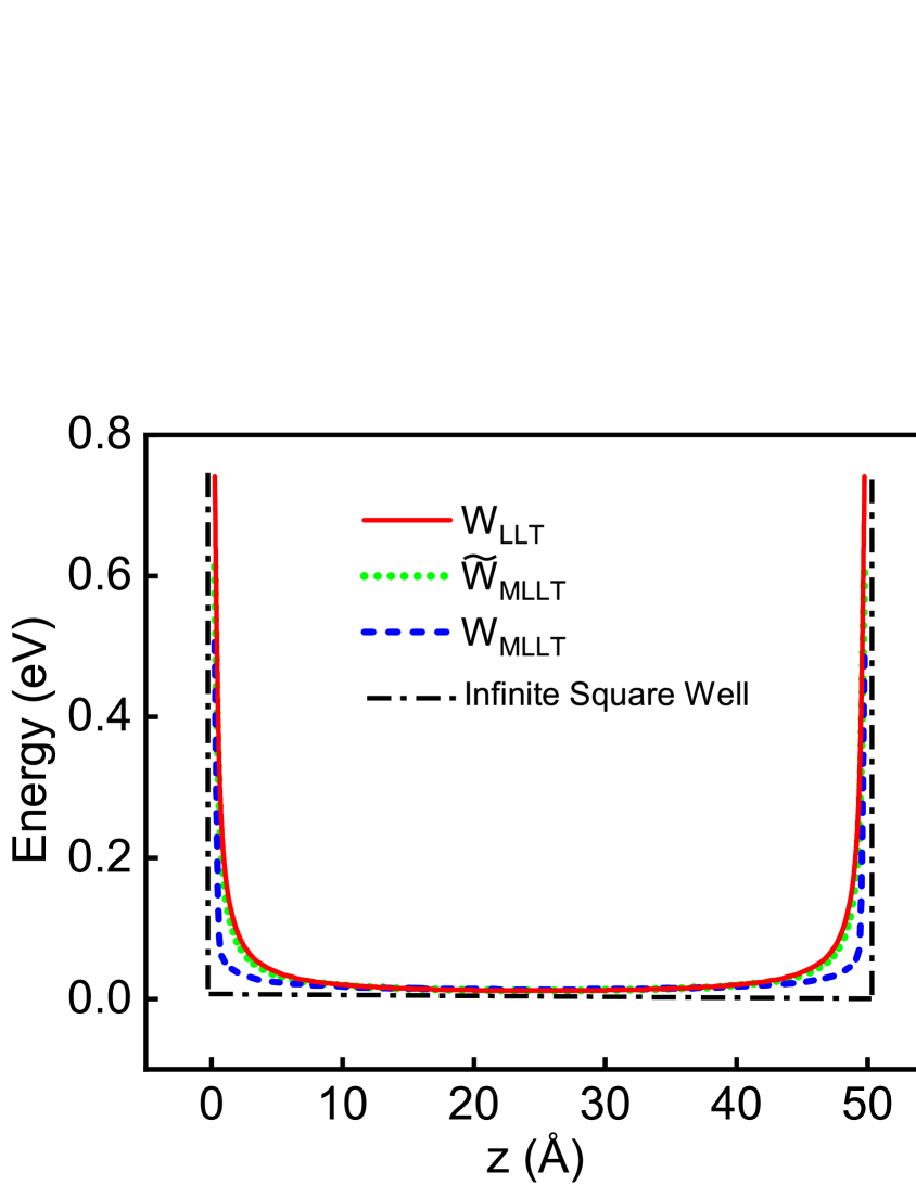
Having discussed energy eigenvalues, we turn now to consider the effective potential resulting from the LLT. This is given by and shown in Fig. 1 by the red solid line along with the potential of a square well (black dashed dotted line) of width 50 Å and with infinitely high barriers. Figure 1 shows that softens the potential near the boundaries. As we will discuss further below, this effect is also seen in a well with finite barriers, where it provides the above discussed quantum corrections to transport simulation. Li et al. (2017) Therefore, it is important that the MLLT captures these pertinent aspects as well, to be of use for such simulations. In the following section we discuss the MLLT for a square well with infinitely high barriers.
III.2 MLLT
Having solved the particle-in-a-box problem within the SE and LLT, we target it now within MLLT by employing:
| (22) |
Using Eq. (4), in the case of the MLLT one is left with
Following the steps outlined above for the LLT, the expansions coefficients , again taking only odd values, are given by
| (23) |
Comparing the above equation with Eq. (18), we find here already that scales as instead of . With this reads:
| (24) |
with . When comparing this result with the expansion of in the LLT frame, Eq. (19), it is evident that the MLLT yields an even faster/better convergence/approximation of with respect to the ground state/fundamental state . Thus, within the MLLT approach the approximation , Eq. (8), should be even better justified.
The square of the energy eigenvalue is given by:
| (25) | ||||
Therefore, yields an even better approximation of the true ground state energy, when compared to the LLT result discussed above (). Again, the reason for this improvement can be traced back to the series expansion of where the expansion coefficients decrease rapidly in magnitude with increasing .
Having seen the improved ground state energy convergence in MLLT, we now turn our attention to the calculation of the effective confining potential within MLLT. In the previous section we have already discussed two approaches to obtain from , namely or . From Eq. (24), it is clear that with will give an effective potential that will be in excellent agreement with , given that . This is confirmed in Fig. 1, where (green dashed line) matches almost perfectly , thus keeping the feature of softening the potential at the infinitely high barriers. Also the second approach, gives a reasonable description of the potential, however, with a less pronounced softening near the barrier.
Overall, we see for the infinite square well potential that gives an effective potential that matches closely , reflecting that each expansion coefficient , cf. Eq. (23), only depends on the ground state energy . However, as indicated already in Sec. II, Eq. (10), this might not be the case for other potentials. We discuss this further briefly in the appendix, where we apply the MLLT to a triangular shaped well with infinitely high barriers. For such a potential we find that LLT does not converge to give a finite estimate of the ground state energy ; MLLT does converge but to an energy that is noticeably different from the solution of the SE. Given that both LLT and MLLT have difficulties in dealing with a triangular shaped potential with infinite barriers, we investigate a triangular shaped well with finite barriers in the following. Such a system is relevant for studying electronic and optical properties of III-N-based QW systems, as we describe in the next section.
| Parameters | GaN | InN | ||
| (eV) | 3.44 | 0.64 | ||
| (Å) | 3.189 | 3.545 | ||
| (Å) | 5.185 | 5.703 | ||
| (C/) | -0.034 | -0.042 | ||
| (C/) | -0.45 | -0.52 | ||
| (C/) | 0.83 | 0.92 | ||
| (GPa) | 106 | 92 | ||
| (GPa) | 398 | 224 | ||
| 0.209 | 0.068 | |||
| 1.876 | 1.811 |
IV Background on nitride-based heterostructures and InGaN Quantum Well
III-N materials, such as InN, GaN and AlN have attracted considerable interest for optoelectronic devices, since their alloys are in principle able to cover emission wavelengths from infrared to deep ultra-violet. Humphreys (2008) InGaN heterostructures, such as QWs, are of particular interest for emission in the visible spectral range. Humphreys (2008) When compared to other III-V materials, such as InAs or GaAs, III-N materials preferentially crystallize in the wurtzite crystal phase while InAs and GaAs crystallize in the zinc blende phase. The wurtzite crystal structure, due to its lack of inversion symmetry, allows for a strain-induced piezoelectric polarization vector field but also a spontaneous polarization vector field, which is even present in the absence of any strain effects. Bernardini et al. (1997) Discontinuities in the polarization vector fields lead to very strong electrostatic built-in fields (MV/cm) in InGaN/GaN QW systems grown along the wurtzite -axis, which is the standard growth direction for these systems. Schwarz and Kneissl (2007); Patra and Schulz (2017) Often these systems, especially when dealing with transport properties of InGaN/GaN MQW-based LED structures, are treated as 1-D systems in which the conduction and valence band profiles are modified by the presence of the intrinsic electrostatic built-in potentials. Schwarz and Kneissl (2007); Caro et al. (2011) It should be noted that this is a simplified description of these systems; more recently it has been shown that the alloy microstructure of InGaN QWs significantly affects the electronic structure, so that local potential fluctuations play an important role. Watson-Parris et al. (2011); Schulz et al. (2015) However, for the analysis here, a simplified 1-D model is a good starting point for comparing LLT and MLLT and to highlight the benefits of the MLLT in terms of convergence and “robustness” of the solution against, for instance, the choice of the sub-region over which is being evaluated to obtain the ground state energy in the given region. Since the methodology of the MLLT is the same as that of the LLT, MLLT can directly be applied to a landscape with energy fluctuations due to alloy fluctuations. However, as discussed already above, further consideration must then be given as to how best to calculate within MLLT, which we will do below. To flesh out the benefits of the MLLT, we focus on the often used 1-D description of the electronic structure of -plane InxGa1-xN/GaN QWs with different In contents . As mentioned above, due to the underlying wurtzite crystal structure and growth along the -axis, -plane InGaN/GaN QW systems exhibit very strong electrostatic built-in fields. This electrostatic field arises from discontinuities in spontaneous and piezoelectric polarization vector fields. The corresponding total built-in potential , assuming that the wurtzite -axis is parallel to the -axis of the coordinate system, can be expressed as: Caro et al. (2011)
| (26) |
Here, is the height/width of the QW with well barrier interfaces at =0 and = . The dielectric constant of the QW material is denoted by and () is the spontaneous polarization in the well (barrier). Assuming that the barrier material is strain-free, a strain field is only present in the InGaN QW, since InGaN has a larger lattice constant than GaN. Vurgaftman and Meyer (2003) Thus one is left with a piezoelectric polarization component in the well , which in the 1-D case can be written as: Schulz et al. (2011)
| (27) |
Here, and are the (well) piezoelectric coefficients and the strain tensor components. The strain tensor components are given by and ; () is the in-plane lattice constant of the well (barrier) material and are the elastic constants of the well material. The material parameters used in this study are summarized in Tab. 1. When calculating the electrostatic built-in potential of InxGa1-xN/GaN QWs as a function of the In content , a linear interpolation of the involved material parameters is applied. We neglect contributions from second-order piezoelectric effects. Patra and Schulz (2017) Using Eq. (IV) and the material parameters from Tab. 1, the resulting built-in potential is similar to that of a capacitor. Caro et al. (2011)
Since we are interested in a general comparison between LLT and MLLT results, we calculate the electronic structure of the above discussed InxGa1-xN/GaN QW systems in the framework of a single-band effective mass approximation for electrons and holes. The confining potential for electrons and holes is then given by the conduction band (CB) and valence band (VB) edge alignment between GaN and InGaN. In Eq. (28) below we assume that the VB edge of bulk GaN (no built-in field) denotes the zero of energy in our system; the GaN CB edge, in the absence of the built-in field, is at the band gap energy of bulk GaN. The InxGa1-xN CB edge, , and the VB edge, , are calculated as a function of the In content as follows: Caro et al. (2013)
| (28) |
Here, is the natural VB offset between pure InN and GaN, which has been taken from HSE-DFT calculations. Moses et al. (2011) The (composition dependent) CB and VB edge bowing parameters are denoted by and . Caro et al. (2013) In combination with the built-in potential from above, the band edge profile shows the well known triangular-shaped profile, leading to the situation that electrons and holes are spatially separated along the growth direction (-axis/-axis). This situation is also know as the quantum confined Stark effect (QCSE). Im et al. (1998)
Building on this potential profile we use a single-band effective mass approximation to construct the Hamiltonian matrix of this system. Here, we use different effective masses for electrons and holes, with the values given in Table 1. A linear interpolation between the effective masses of InN and GaN has been applied to obtain the corresponding masses for InGaN. However, differences in the effective mass inside and outside the well are not considered. Given that we are interested in ground state energies and more generally in a comparison between results obtained from the SE, LLT and MLLT, applying a constant effective mass should be sufficient for our purposes here. To numerically solve , and we use the finite difference method and assume a well of width of Å with a barrier width of Å on each side of the well; the discretization step size is Å.
V Results for -plane N/GaN quantum wells
In this section we compare and discuss ground state energies, wave functions and the effective potential of -plane InxGa1-xN/GaN QWs obtained by solving SE, LLT and MLLT in the numerical framework discussed above. Special attention is paid to the impact of the In content on the results, given that with increasing In content the piezoelectric contribution to the built-in potential, and thus the “tilt” in the band edge profiles, increases. More specifically, we study here In contents ranging from 5% up to 50%, even though the very high In contents () are experimentally very difficult to achieve for fully strained -plane wells. Such an analysis will help us to compare the impact of strong asymmetries in the potential landscape on the results of the LLT and MLLT, respectively. Strong fluctuations in the potential landscape may occur locally in InGaN QWs with higher In contents (e.g. 25% In) due to random alloy fluctuations.
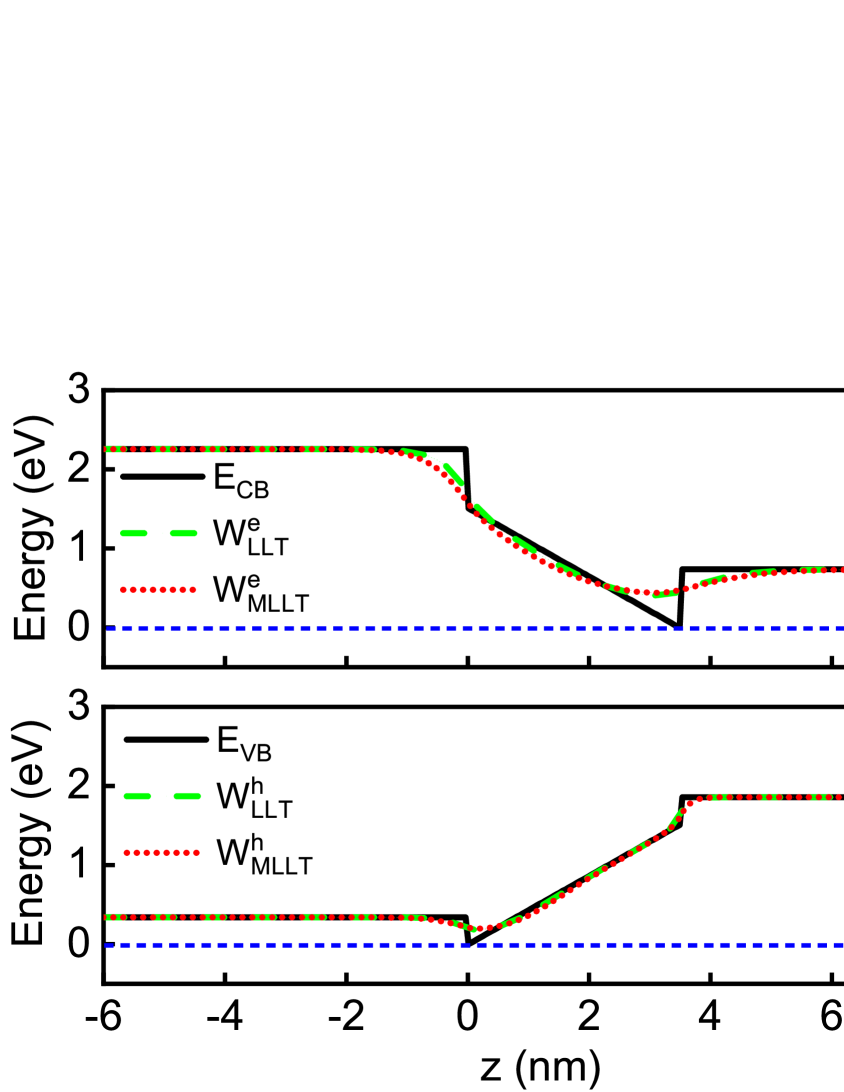
Several aspects of the following analysis are to be noted. Firstly, the solution of the SE represents the reference/benchmark for the results of LLT and MLLT. Secondly, since we are using a single-band effective mass approximation in the framework of a finite difference method, we treat electrons and holes separately. In doing so, especially for LLT and MLLT, care must be taken when defining the zero of energy. As discussed in Sec. II, the expansion coefficients for constructing from the eigenstates of the system are inversely proportional to the corresponding state energies. Ideally, the zero of energy should be chosen close to the “true” ground state energy of the system in a given subregion . By doing so, the expansion coefficient is then large as compared to higher order terms that have lesser contributions. As a consequence is then a very good approximation of the ground state wave function, resulting also in a good estimate of the corresponding energy. Here, we always choose the zero of energy as the minimum energy in the band edge profile of the confining potential for electrons and holes. An illustration of this situation is displayed in Fig. 2.
Finally, following Eq. (9), when calculating the ground state energy from , the subspace region over which is integrated has to be chosen. To illustrate the impact of on the results, three different subregions have been considered for electrons and holes. For electrons these are labeled as , and . The first electron subregion, , corresponds to the entire simulation cell (-10 nm to 13.5 nm). The subregion considers slightly more than the QW region, i.e. -1.5 nm 5 nm. For the last subregion, , we just consider it to be 0 nm 4.5 nm, meaning that this region starts at the well-barrier interface at and extends 1 nm into the barrier region above the upper QW interface at nm. This asymmetry in accounts for the tilt in the band edges and that therefore the electron wave function is expected to leak further into the barrier region on the -side of the well. For holes, the subregions one and two are identical to the first two electron cases. Only subregion is different from . For we have chosen -1 nm 3.5 nm, which reflects that the tilt in the band edges shifts electron and hole states in opposite directions.
The aim of using these three different subregions is twofold. First, as mentioned already above, it will allow us to analyze the impact of the subregion choice on the ground state energies obtained from LLT and MLLT in comparison to the result obtained from solving the SE. Secondly, this analysis also enables us to study if the choice of affects differently the results obtained from LLT and MLLT. This insight is for instance of interest when treating (random) potential fluctuations, where partitioning the system may be difficult. Thus, a method where results are less dependent on the choice is in general preferred.
V.1 Electron ground state energies, wave functions and effective potential
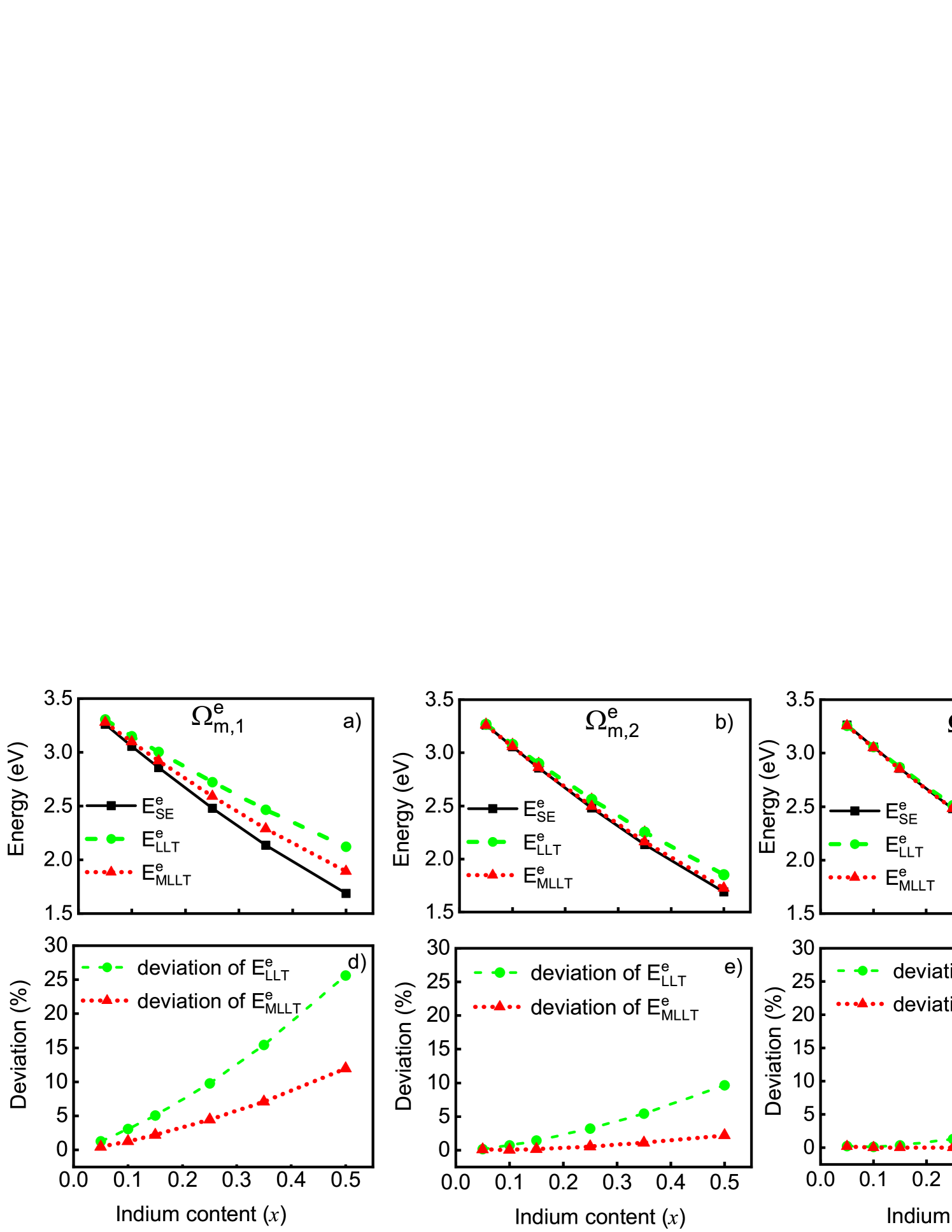
In a first step we focus on the results for the electron ground state energy as a function of the In content for the above discussed -plane InxGa1-xN/GaN QWs. The data are presented in Fig. 3, upper row, for the three different integration regions . The results obtained by solving the SE, , are given by the black squares. The green circles show the results from LLT, , while the red triangles denote MLLT data. Before looking at the results in detail, one can already infer from Fig. 3 that when using subregion , cf. Fig. 3 c), a very good agreement between LLT, MLLT and SE is achieved. Clearly larger deviations are observed for LLT and MLLT with respect to the SE result when using the full simulation cell, , cf. Fig. 3 a).
The lower row of Fig. 3 displays the deviations (in %) between LLT (MLLT) and the solution of the SE as a function of the In content for the three different subregions . The green circles show the data for the comparison between the SE and LLT, while the red triangles do so for the comparison between SE and MLLT. Starting with , Fig. 3 d), we observe that for both LLT and MLLT the deviations increase with increasing In content in the well. However, LLT shows noticeably larger deviations when compared to MLLT for In contents exceeding values of 15% (). Turning to , Fig. 3 e), deviations are in general strongly reduced. Nevertheless, still a noticeable difference between LLT and MLLT is observed. More specifically, while LLT produces errors of above 5%, the MLLT results are a good approximation of the true ground state energy, independent of the In content (errors below 2% are found). When restricting the integration region further (), Fig. 3 f), deviations in LLT are further reduced and only in the very high In content regime () more pronounced deviations are observed. The error in the MLLT result is below 1% over the range of In composition considered. This analysis shows that the MLLT produces a better approximation of the electron ground state energy, independent of the In content and chosen subregion . This makes it therefore very attractive for calculations of the fundamental state in subregion of an energy landscape which shows strong fluctuations so that the system cannot be easily partitioned into different subregions.
This begs the question why the energy obtained from MLLT is more robust against changes in . To address this point, Fig. 4 shows the (normalized) electron ground state wave function calculated from the SE (black solid line) and the (normalized) functions obtained from LLT (green dashed line) and MLLT (red dotted line) using the full simulation box . The results are displayed for the -plane In0.25Ga0.75N/GaN QW. The electron ground state wave function shows the expected behavior of having the highest value in the QW region, with the wave function amplitude then decaying rapidly in the GaN barrier region. Turning to the result from LLT (green dashed line) first, we find that has a maximum in the well, however, it has also a constant finite value in the GaN barrier region, especially for nm. Thus when changing the integration region , a strong impact on the obtained energy could be expected since contributions from in the barrier are removed when reducing the subregion . This is exactly the situation we observe in Fig. 3. More specifically changing the subregion from (full system) to (mainly QW region), the error in when compared to , reduces from 9.8% to 1.3% for the In0.25Ga0.75N/GaN QW.
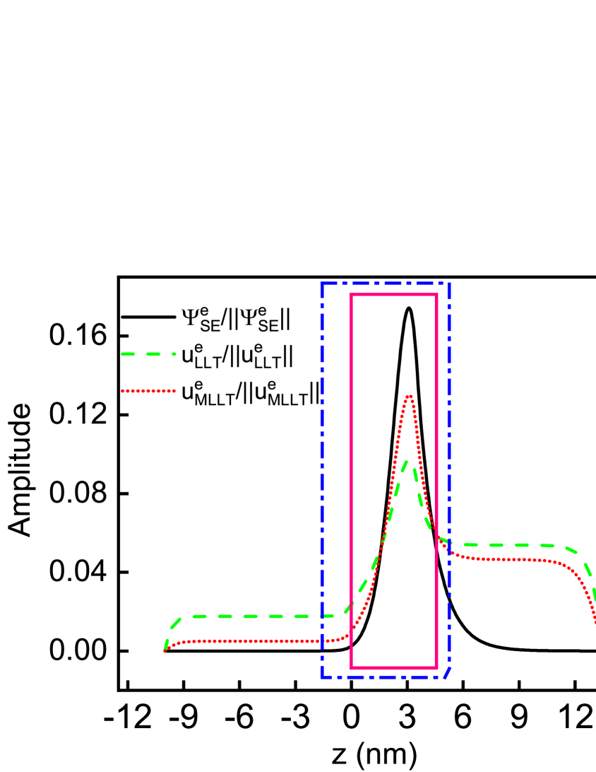
The situation is different in the MLLT approach. Here, , at least for nm, gives a better approximation of , with the magnitude of being very small, similar to but in contrast to . However, for nm the magnitude of is comparable to that of and therefore much larger than in this region. Thus, given that the magnitude of is small in the region nm and shows to be a good approximation of in the QW region, the analysis confirms the observation that is less dependent on than .
Finally, we discuss here the effective confining potential for electrons obtained both within LLT, , and MLLT, . In case of LLT it is obtained via , and given in Fig. 2 a) by the green dashed line for an InGaN/GaN QW with 25% In. The potential reveals a softening at the QW barrier interface, which, as discussed above, is an important feature for quantum corrections in drift-diffusion calculations using for the energy landscape. The here observed potential profile is consistent with the results reported previously. Filoche et al. (2017) To obtain the effective confining potential from MLLT that reflects the behavior of , we find that works here best, while results in a very different effective potential from (not shown). Figure 2 a) confirms that (red dotted line) is in very good agreement with (green dashed line). We note that this holds over the full In content range studied here.
V.2 Hole ground state energies, wave functions and effective potential
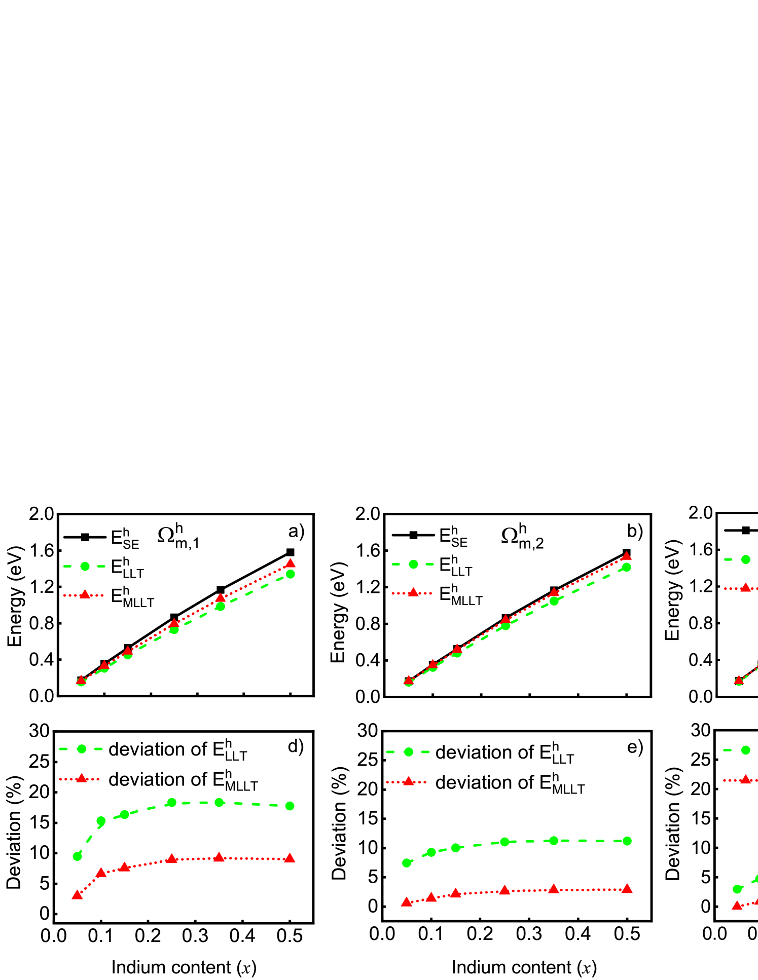
Having discussed the results for the electron ground state energies, wave functions and the effective confining potential, we now turn and present the results for holes, again as a function of the In content for the above discussed -plane InxGa1-xN/GaN QWs. The upper row of Fig. 5 presents the comparison between the energies obtained from SE, (, black squares), LLT, (, green circles) and MLLT, (, red triangles). The results are shown for the three different subregions over which is integrated to obtain the corresponding energy. The lower row of Fig. 5 depicts for the deviation (in %) of LLT (green circles) and MLLT (red triangles) from the SE solution. Looking at Fig. 5 a) first, one can clearly see that when integrating over the full simulation region (), both and deviate from with increasing In content . However, deviations are larger for LLT than for MLLT. A similar behavior was also observed for the electron ground state energies when the full simulation box is considered, cf. Fig. 3. But, trends for electrons and holes are quite different. For electrons, the deviation in the ground state energies with respect to the SE solution increase with increasing In content , cf. Fig. 3 d). For the holes, deviations in the ground state energy also start to increase with increasing In content but deviations saturate at around 18% and 8% for LLT and MLLT, respectively, when the In content exceeds 15% (). This analysis shows, similar to the results for the electrons, that when using the full simulation cell (), MLLT provides a better description of when comparing errors with LLT. When adjusting/reducing the subregion , cf. Figs. 5 b) and c), to calculate and , the agreement with clearly improves. This is in particular true for , as Fig. 5 e) and f) show; deviations from close to 3% or less are observed over the full In content range . More specifically, for a well with 25% In, the error in reduces from 8% to 1.8% (see Figs. 5 d) and f)) when changing from to . Looking at for the same situation, we observe that the deviations are reduced from 18.4% () to 8% (). However, the values are still noticeably higher when compared to . This also shows that MLLT results are robust against changes in the In content , while LLT exhibits larger deviations from the SE data, especially for higher In contents.
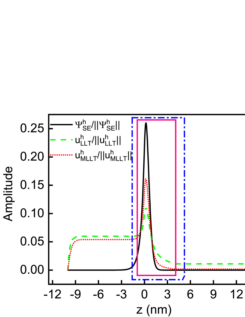
Following our investigations on the electron ground state energies and wave functions, we study here also the hole ground state wave functions. Again we use as a test system the -plane In0.25Ga0.75N/GaN QW. The wave functions calculated from SE (black solid line), LLT (green dashed line) and MLLT (red dotted line) are shown in Fig. 6. Before looking at the fine details, independent of the model used, the wave functions are localized inside the well and “decay” in the GaN barrier region. However, how the wave functions decay in the barrier region strongly depends on the model. While the hole ground state wave function rapidly decays in the barrier material, this situation is only true for and along the -direction. Even though in the -direction and are similar, there are also differences. While is very close to 0 in the barrier region, is small, but has a noticeable finite constant value in the GaN barrier for nm. This effect is amplified for nm. Again and similar to the electrons, we attribute differences in the hole ground state energies to differences in calculated from MLLT and LLT, given that deviations in the ground state energy increase as integration region is increased.
In the last step we turn attention to the effective potential for holes, , calculated within LLT and MLLT. The results are shown in Fig. 2 b). The confining potential from LLT, , is given by the green dashed line and shows again a softening of the potential near the well barrier interface. Also for holes we have tested calculating the effective potential from MLLT via and . The conclusion that is drawn from this is similar to that for electrons, meaning that gives a potential profile very different from (not shown), while is in good agreement with . This is confirmed by Fig. 2 b), showing that the confining potential obtained from MLLT (red dotted line) captures the same effects as (green dashed line). Again this result holds over the full In content range investigated here.
VI Conclusions
In this work we have proposed, motivated and analyzed, a modified localization landscape theory (MLLT). In the MLLT approach we solve instead of , as in the LLT. We demonstrate the improvements resulting from using in predicting ground state energies for a particle-in-a-box (infinite square well) potential. Since this problem can be solved fully analytically in LLT and MLLT, the solution confirms that obtained from MLLT will in general give a better approximation of the true ground state wave function when compared to the result from LLT. We have also shown that this can be traced back to the energy dependence of the expansion coefficients of in terms of the particle-in-a-box eigenstates. Given that obtained from MLLT provides a very good description of the ground state wave function, it also provides an improved estimate of the ground state energy and therefore the error in this quantity is reduced in comparison to the LLT obtained value. Here, we also have provided insight into the calculation of the effective confining potential within MLLT. While this is straightforward in the case of a particle-in-a-box problem with infinitely high barriers, we highlight that care must be taken when extracting the effective confining from MLLT in general. We have discussed two strategies to obtain from MLLT that lead to results similar to those obtained from LLT, which is important when applying MLLT for instance in drift-diffusion transport calculations to account for quantum corrections.
The particle-in-a-box problem provided the ideal testbed to study the basic properties of the LLT and MLLT. However, further analysis is required to consider more realistic potentials. LLT has recently been used to evaluate the electronic structure of III-N heterostructures, where the confining potential is triangular shaped with barriers of finite height. Motivated by this, we have studied and compared ground state energies from the Schrödinger equation (SE), LLT and MLLT for -plane InxGaxN/GaN QWs as a function of the In content . Special attention was paid to the impact of the choice of the integration region of when evaluating the ground state energies. Our calculations reveal that for both electron and hole ground states, MLLT always gives a better description of the “true” ground state energy when compared to the LLT result. We also find that the subregion over which is being integrated to obtain this energy is less important for MLLT than it is for LLT. Over the composition range from 5% to 50% In in the well and when integrating over a region close to the QW, errors in the ground state energy from MLLT never exceeds 4%. While similar numbers are obtained for LLT in the lower In content range (15% In) and when choosing appropriate subregions, especially for holes at higher In contents (25% In), errors in the range of 5% to 10% are observed. Looking at the calculated effective potential for electrons and holes, and independent of the In content , we find that using gives in general results that match closely the effective potential obtained from LLT. Since plays an important role in quantum corrected drift-diffusion simulations, it is useful to see that MLLT produces an energy landscape similar to LLT, so that it can be used in such simulations.
Taking all this together the proposed MLLT keeps all the benefits of the LLT, such that only a system of linear equations has to be solved instead of a large eigenvalue problem to obtain ground state energies. At the same time the MLLT provides the following aspects: (i) “faster convergence” of the calculated ground state energies with integration region, (ii) a more “robust” behavior of the method against changes in the integration region, (iii) better agreement with results from SE, especially for higher In contents and (iv) an effective confining potential comparable to that of LLT. All these features make the MLLT method attractive for calculations of localized states in highly disordered systems, where for instance partitioning the systems into different subregions is not trivial.
Acknowledgements.
The authors acknowledge financial support from Science Foundation Ireland under Grant Nos. 17/CDA/4789, 15/IA/3082 and 12/RC/2276 P2.*
Appendix A Infinite Triangular Well
Having discussed in the main text the fully analytic solution of the particle-in-a-box problem with infinitely high barriers, we study here another problem that can be investigated fully analytically, which is a triangular well with infinitely high barrier at ; the potential increases from at with a slope in the +-direction. The aim of this study is twofold: it will illustrate (i) that in contrast to the particle-in-a-box problem, discussed in Sec. III, the expansion coefficients of can depend on multiple energies and (ii) that there are potentials where LLT and MLLT could fail to give a good approximation of (ground state) energies or even diverge. Regarding (i), this finding is important for calculating the effective confining potential, showing that it might not always be guaranteed that calculating will give a good approximation of obtained from the “standard” LLT approach.
For the infinite triangular potential, the SE reads:
| (29) |
Setting and using , one is left with
| (30) |
The general solution to the above differential equation can be obtained as a linear combination of the Airy functions and . These functions are defined as the improper Riemann integrals Vallee and Soares (2004)
| (31) |
| (32) |
For , the function shows exponential decay whereas diverges to infinity. Given that the confined wave functions have to decay as , the function has to be discarded. Thus, the solutions of the SE for a triangular-shaped potential with infinitely high barriers, cf. Eq. (29), are given by:
| (33) |
The fact that the wave function has to go to zero at the infinitely high barrier at can be used to determine the energy eigenvalues . To do so, the th zero of the Airy function is approximated and the corresponding eigenvalue then reads:
| (34) |
Equipped with this solution we turn now and discuss the infinite triangular well firstly in the framework of LLT and then of MLLT. To find a series expansion for , we first need an expansion for the constant function 1 in terms of the eigenfunctions, over the interval [0, ): Abramowitz and Stegun (2004)
| (35) |
We recall here that , Eq. (4), so that when using LLT, , one is left with
| (36) |
Due to the orthonormality of the wave functions, we can thus express the expansion coefficients as
| (37) |
Thus, within LLT, can be expressed as:
| (38) |
In contrast to the infinite square-well potential, one can show that the sum of the ’s does not converge for the triangular well considered and thus the energy ,Eq. (9), does not converged. First, we note that the energies , Eq. (34), increase with increasing as ; numerical analysis we have undertaken indicates that decays approximately as , where ; hence in LLT decays approximately as , where , which results in a divergent series for , Eq. (4).
Turning to the MLLT, and following the same procedure as for the LLT, we find here that the coefficients are given by
| (39) |
Successive terms in the series Eq. (39) decay as . Therefore, higher order term contributions are reduced in the MLLT case. Numerical studies confirm that MLLT converges with increasing system size, in contrast to the LLT. However, MLLT converges to a ground state energy that is noticeably larger than the ground state energy obtained from SE. All this highlights benefits but also potential shortcomings or problems in both LLT and MLLT for certain potentials.
References
- Dierks and Czycholl (1998) H. Dierks and G. Czycholl, J. Cryst. Growth 185, 877 (1998).
- Stier et al. (1999) O. Stier, M. Grundmann, and D. Bimberg, Phys. Rev. B 59, 5688 (1999).
- Fry et al. (2000) P. W. Fry, I. E. Itskevich, D. J. Mowbray, M. S. Skolnick, J. J. Finley, J. A. Barker, E. P. O’Reilly, L. R. Wilson, I. A. Larkin, P. A. Maksym, et al., Phys. Rev. Lett. 84, 733 (2000).
- Baer et al. (2004) N. Baer, P. Gartner, and F. Jahnke, Eur. Phys. J. B 42, 231 (2004).
- Christmas et al. (2005) U. M. E. Christmas, A. D. Andreev, and D. A. Faux, J. Appl. Phys. 98, 073522 (2005).
- Winkelnkemper et al. (2006) M. Winkelnkemper, A. Schliwa, and D. Bimberg, Phys. Rev. B 74, 155322 (2006).
- Schliwa et al. (2007) A. Schliwa, M. Winkelnkemper, and D. Bimberg, Phys. Rev. B 76, 205324 (2007).
- Marquardt et al. (2008) O. Marquardt, D. Mourad, S. Schulz, T. Hickel, G. Czycholl, and J. Neugebauer, Phys. Rev. B 78, 235302 (2008).
- Singh and Bester (2009) R. Singh and G. Bester, Phys. Rev. Lett. 103, 063601 (2009).
- Schulz et al. (2015) S. Schulz, M. A. Caro, C. Coughlan, and E. P. O’Reilly, Phys. Rev. B 91, 035439 (2015).
- Andreev et al. (2012) Z. Andreev, F. Römer, and B. Witzigmann, Phys. Stat. Solidi A 209, 487 (2012).
- Piccardo et al. (2017) M. Piccardo, C.-K. Li, Y.-R. Wu, J. S. Speck, B. Bonef, R. M. Farrell, M. Filoche, L. Martinelli, J. Peretti, and C. Weisbuch, Phys. Rev. B 95, 144205 (2017).
- Piprek (2017) J. Piprek, ed., Handbook of Optoelectronic Device Modeling & Simulation, Series in Optics and Optoelectronic (CRC Press, Taylor & Francis Group, Boca Raton, 2017).
- Bester et al. (2003) G. Bester, S. Nair, and A. Zunger, Phys. Rev. B 67, 161306(R) (2003).
- Li et al. (2017) C.-K. Li, M. Piccardo, L.-S. Lu, S. Mayboroda, L. Martinelli, J. Peretti, J. S. Speck, C. Weisbuch, M. Filoche, and Y.-R. Wu, Phys. Rev. B 95, 144206 (2017).
- Filoche and Mayboroda (2012) M. Filoche and S. Mayboroda, PNAS 109, 14761 (2012).
- Arnold et al. (2016) D. N. Arnold, G. David, D. Jerison, S. Mayboroda, and M. Filoche, Phys. Rev. Lett. 116, 056602 (2016).
- Filoche et al. (2017) M. Filoche, M. Piccardo, Y.-R. Wu, C.-K. Li, C. Weisbuch, and S. Mayboroda, Phys. Rev. B 95, 144204 (2017).
- Chalopin et al. (2019) Y. Chalopin, F. Piazza, S. Mayboroda, C. Weisbuch, and M. Filoche, Sci. Rep. 9, 12835 (2019).
- Lemut et al. (2019) G. Lemut, M. J. Pacholski, O. Ovdat, A. Grabsch, J. Tworzydlo, and C. W. J. Beenakker, arXiv:1911.04919 [cond-mat.mes-hall] (2019).
- Schulz and O’Reilly (2017) S. Schulz and E. P. O’Reilly, Chapter 1: Electronic band structure, Handbook of optoelectronic devices modeling and simulation, Vol. 1, Series in Optics and Optoelectronic (CRC Press, 2017).
- Caro et al. (2013) M. A. Caro, S. Schulz, and E. P. O’Reilly, Phys. Rev. B 88, 214103 (2013).
- Wojs et al. (1996) A. Wojs, P. Hawrylak, S. Fafard, and L. Jacak, Phys. Rev. B 54, 5604 (1996).
- Bester (2009) G. Bester, J. Phys.: Condens. Matter 21, 023202 (2009).
- Kindel et al. (2010) C. Kindel, S. Kako, T. Kawano, H. Oishi, Y. Arakawa, G. H nig, M. Winkelnkemper, A. Schliwa, A. Hoffmann, and D. Bimberg, Phys. Rev. B 81, 241309 (2010).
- Patra and Schulz (2017) S. K. Patra and S. Schulz, Phys. Rev. B 96, 155307 (2017).
- Wang and Zunger (1994) L.-W. Wang and A. Zunger, J. Chem. Phys. 100, 2394 (1994).
- Nolting (2017) W. Nolting, Theoretical Physics 6 – Quantum Mechanics – Basics (Springer International Publishing, Cham, Switzerland, 2017).
- Fogiel (1991) M. Fogiel, The Advanced Calculus Problem Solver (Research and Education Association, New Jersey, 1991).
- Arnold et al. (2019) D. Arnold, G. David, M. Filoche, D. Jerison, and S. Mayboroda, SIAM J. Sci. Comput. 41, B69 (2019).
- Caro et al. (2011) M. A. Caro, S. Schulz, S. B. Healy, and E. P. O’Reilly, J. Appl. Phys. 109, 084110 (2011).
- Rinke et al. (2008) P. Rinke, M. Winkelnkemper, A. Qteish, D. Bimberg, J. Neugebauer, and M. Scheffler, Phys. Rev. B 77, 075202 (2008).
- Schulz et al. (2010) S. Schulz, T. J. Badcock, M. A. Moram, P. Dawson, M. J. Kappers, C. J. Humphreys, and E. P. O’Reilly, Phys. Rev. B 82, 125318 (2010).
- Humphreys (2008) C. J. Humphreys, MRS Bulletin 33, 459 (2008).
- Bernardini et al. (1997) F. Bernardini, V. Fiorentini, and D. Vanderbilt, Phys. Rev. B 56, R10024 (1997).
- Schwarz and Kneissl (2007) U. T. Schwarz and M. Kneissl, Phys. Stat. Sol. (RRL) 1, A44 (2007).
- Watson-Parris et al. (2011) D. Watson-Parris, M. J. Godfrey, P. Dawson, R. A. Oliver, M. J. Galtrey, M. J. Kappers, and C. J. Humphreys, Phys. Rev. B 83, 115321 (2011).
- Vurgaftman and Meyer (2003) I. Vurgaftman and J. R. Meyer, J. Appl. Phys. 94, 3675 (2003).
- Schulz et al. (2011) S. Schulz, M. A. Caro, E. P. O’Reilly, and O. Marquardt, Phys. Rev. B 84, 125312 (2011).
- Moses et al. (2011) P. G. Moses, M. Miao, Q. Yan, and C. G. Van de Walle, J. Chem. Phys. 134, 084703 (2011).
- Im et al. (1998) J. S. Im, H. Kollmer, J. Off, A. Sohmer, F. Scholz, and A. Hangleiter, Phys. Rev. B 57, R9435 (1998).
- Vallee and Soares (2004) O. Vallee and M. Soares, Airy functions and applications to physics (Imperial College Press, London, 2004).
- Abramowitz and Stegun (2004) M. Abramowitz and I. Stegun, Handbook of Mathematical Functions, Applied Mathematics Series (National Bureau of Standards, Washington, D. C., 2004).