Elucidating Flow Matching ODE Dynamics with Respect to Data Geometries

Zhengchao Wan Co-first author. zwan@missouri.edu Department of Mathematics, University of Missouri Qingsong Wang Co-first author. qswang92@gmail.com Halıcıoğlu Data Science Institute, University of California San Diego Gal Mishne gmishne@ucsd.edu Halıcıoğlu Data Science Institute, University of California San Diego Yusu Wang yusuwang@ucsd.edu Halıcıoğlu Data Science Institute, University of California San Diego

Abstract

Diffusion-based generative models have become the standard for image generation. ODE-based samplers and flow matching models improve efficiency, in comparison to diffusion models, by reducing sampling steps through learned vector fields. However, the theoretical foundations of flow matching models remain limited, particularly regarding the convergence of individual sample trajectories at terminal time—a critical property that impacts sample quality and being critical assumption for models like the consistency model. In this paper, we advance the theory of flow matching models through a comprehensive analysis of sample trajectories, centered on the denoiser that drives ODE dynamics. We establish the existence, uniqueness and convergence of ODE trajectories at terminal time, ensuring stable sampling outcomes under minimal assumptions. Our analysis reveals how trajectories evolve from capturing global data features to local structures, providing the geometric characterization of per-sample behavior in flow matching models. We also explain the memorization phenomenon in diffusion-based training through our terminal time analysis. These findings bridge critical gaps in understanding flow matching models, with practical implications for sampling stability and model design.

1 Introduction

Diffusion-based generative models have become the de facto standard for the task of image generation [SDWMG15, HJA20, SE19]. Compared to previous generative models (e.g., GANs [GPAM⁺14]), diffusion models are easier to train but suffer from long sampling times due to the sequential nature of the sampling process. To address this limitation, (deterministic) ODE-based samplers were introduced, where the sampling process is done by integrating an ODE trajectory. This approach has been shown to be more efficient than traditional sampling with a significantly reduced number of sampling steps needed [SME21, LZB⁺22, KAAL22]. Recently, a new class of models, known as flow matching models [LCBH⁺22, LGL23] has been developed to use an ODE flow map to interpolate between a prior and a target data distribution—generalizing diffusion models with ODE samplers. By learning a vector field $u_{t}$ a new sample $x_{1}$ can be generated by integrating over the ODE below from some initial random sample $x_{0}$ :

\frac{dx_{t}}{dt}=u_{t}(x_{t}),\,t\in[0,1].

Various versions of the flow matching model have gained popularity, such as the rectified flow model [LGL23], which is used in recent commercial image generation software [EKB⁺24]. Furthermore, the succinct and deterministic formulation of the flow matching model also makes theoretical analysis potentially easier.

However, despite their empirical success, the theoretical understanding of flow models remains incomplete, even for the well-posedness of the ODE trajectories, i.e., existence, uniqueness, as well as convergence as $t\to 1$ of the ODE trajectories. These are not thoroughly addressed in the pioneering papers [LCBH⁺22, LGL23], and only partially tackled in recent studies [GHJ24, LHH⁺24]. Specifically, in [LHH⁺24], well-posedness is established only on the open interval $[0,1)$ . Recent work [GHJ24] extend well-posedness to $[0,1]$ but under restrictive assumptions on the data distribution, excluding cases where data is supported on low-dimensional manifolds—an arguably crucial scenario in generative modeling [LGRH⁺24]. In both works, the challenge arises from the singularity in the vector field $u_{t}$ as the terminal time $t=1$ is approached, influenced by both the ODE formulation and the data geometry. The convergence of the ODE trajectories lies in a broader context of sample trajectory analysis, which is less explored in the literature as most work focuses on distribution level analysis [BDD23, LC24].

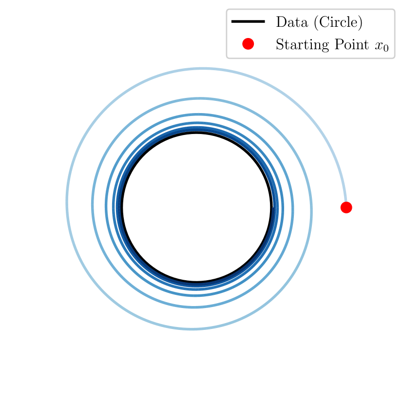
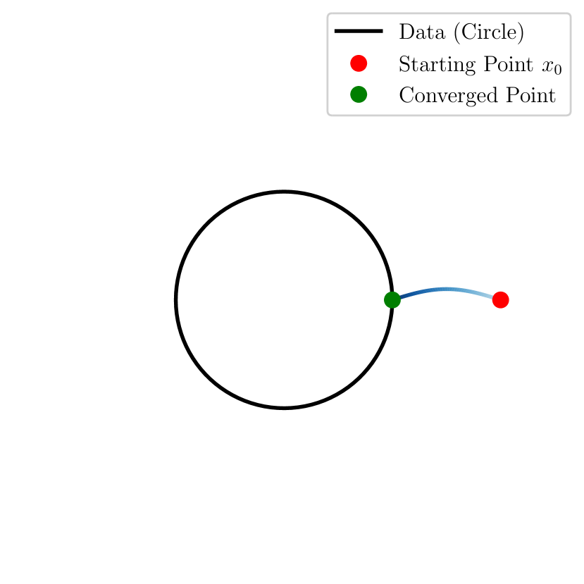
Refer to caption — (a) An ODE trajectory that winds towards the data distribution without convergence as $t\to 1$ .

We also highlight that pushing the well-posedness to $t=1$ and performing sample trajectory analysis is not only theoretically interesting but also of practical importance. Suppose we know that the ODE trajectory exists in $[0,1)$ , and the intermediate distribution following the ODE flow is getting closer to the data distribution as $t$ increases. However, if the ODE trajectory does not converge at $t=1$ , the final sampling following a single ODE trajectory can be very sensitive to the chosen ODE discretization scheme, i.e., a slight change in sampling schedule will result in a drastically different outcome. This could happen if the individual ODE trajectories are winding towards the data distribution but never converge at $t=1$ as shown in Figure 1(a). A more desirable behavior is as in Figure 1(b), where the ODE trajectory converges to the data distribution as $t\to 1$ . Empirical studies find the ODE trajectories tend to stabilize as $t\to 1$ and hence be more aligned with that of Figure 1(b), and this observation is utilized to guide the choice of the ODE discretization scheme [KAAL22, EKB⁺24]. Furthermore, the convergence of the ODE trajectories at $t=1$ is a critical assumption for the consistency model [SDCS23], which utilizes the limit of the ODE trajectory to design a one-step diffusion model. These considerations motivate us to investigate the convergence of the ODE trajectories at $t=1$ and per sample trajectory analysis.

In this paper, our approach focuses on the denoiser, a key component of flow matching models. The denoiser, defined as the mean of the posterior distribution of the data given a noisy observation, governs the evolution of ODE trajectories. Initially, the posterior distribution is broad, and the denoiser approximates the global mean of the data. As time progresses, the posterior measure becomes more concentrated around nearby data points, and the denoiser captures finer details of the data distribution.

We show that when approaching the terminal time, the posterior distribution concentrates on the nearest data, and the denoiser converges to the projection of the current sample onto the data support. This extends previous partial results [PY24, SBDS24] to a general setting beyond a small neighborhood of the data support. By carefully leveraging this denoiser convergence and integrating it with the analysis of the ODE dynamics, we find that near the terminal time, the ODE trajectories will stay in a region away from the singularity and converge to the data support. As a result, we establish the convergence of the entire sampling process with minimal assumptions and validate that the ODE trajectories in flow matching models are well-behaved (as in Figure 1(b)).

Notably, the terminal time analysis of the denoiser provides a new perspective on the memorization phenomenon observed in diffusion-based training where models only repeat the training samples [CHN⁺23, WLCL24], rather than generate new unseen data points. We identify that the denoiser’s terminal time convergence to the data support precisely leads to this memorization behavior. In particular, if a neural network trained denoiser is asymptotically trained optimally with empirical data, it can only sample memorized training data.

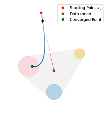
Finally, our analysis significantly strengthens the understanding of flow matching ODE dynamics, extending beyond the terminal time. By carefully examining the progressive concentration of the posterior distribution, we derive comprehensive insights into the behavior of ODE trajectories. Specifically, we establish a unified result demonstrating that trajectories are systematically attracted to, and ultimately absorbed by, sets associated with the data distribution. Initially, sample trajectories move towards the mean of the data distribution and will be absorbed into the convex hull of overall data distribution, capturing the global structure. As the process evolves, they are increasingly drawn towards local clusters within the data, reflecting a transition from global to local convergence. Ultimately, the trajectories converge to the data support at the terminal time, providing a geometric characterization of how samples naturally focus on local features; see Figure 2 for an illustration. In this way, we provide per sample trajectory analysis that complements the empirical, or distribution level discussion regarding the flow matching/diffusion model dynamics [BBDBM24, LC24].

Figure 3: Illustration of main theoretical results. Our findings are divided into two main parts: the first focuses on the theoretical foundations of flow matching ODEs, emphasizing properties of denoisers and posterior distributions; the second builds on these insights to characterize the three stages of flow matching ODE trajectories. In the first part, we highlight that the well-posedness result serves as the cornerstone for understanding the absorbing and attracting properties of denoisers. Furthermore, leveraging the well-posedness at

t=1

, we establish the existence of the flow map

\Psi_{t}

t=1

, which enables us to derive key properties of flow maps.

Contributions and Organization.

In summary, we provide a comprehensive theoretical analysis of flow matching models by examining the behavior of denoisers and posterior distributions. We establish the convergence of ODE trajectories and characterize their geometric evolution, bridging key gaps in the theoretical understanding of these models. Our results address critical challenges related to terminal time singularities and offer new insights into the memorization phenomenon in diffusion-based training. The geometric perspective we develop—showing how trajectories evolve from global to local features—provides a unified framework for understanding flow matching dynamics, laying a foundation for future theoretical developments. The paper is structured as follows, and Figure 3 provides an illustration of the main theoretical results and their inter-dependencies.

•

In Section 2, we introduce the background on flow matching models, their training objectives, and the unification of different scheduling functions via the noise-to-signal ratio $\sigma$ .
•

In Section 3, we discuss key properties of the denoiser and highlight its role as the guiding component in the flow matching model ODE dynamics, illustrating terminal time singularity and general attracting and absorbing properties. These will be fundamental tools for our theoretical analysis.
•

In Section 4, we study the concentration and convergence of the posterior distribution, establishing its initial closeness to the data distribution and its convergence to the data support at the terminal time. We also derive specific convergence rates under different data geometries.
•

In Section 5, we present the well-posedness of ODE trajectories fisrt in $[0,1)$ and then extend to $[0,1]$ with minimal assumptions on the data distribution. We then obtain refined convergence results based on data geometry. Lastly, with the existence of flow maps, we analyze its equivariance property under data transformation.
•

In Section 6, we analyze the ODE trajectories across different stages, demonstrating their initial attraction to the data mean and eventual absorption into the convex hull of the data distribution. Later, these trajectories are attracted to local clusters. We also provides quantitative results on the terminal time behavior for discrete data distributions and showcase the importance of terminal time behavior on the memorization phenomenon.

All technical proofs are deferred to the appendix.

2 Background on Flow Matching Models

In this section, we provide a brief overview of flow matching models and their training objectives and how the noise-to-signal ratio $\sigma$ can be used to unify different scheduling functions.

2.1 Preliminaries and notations

We use $\mathbb{R}^{d}$ to denote the $d$ -dimensional Euclidean space, and $\|\cdot\|$ to denote the Euclidean norm. We use $\Omega$ to denote a general closed subset $\Omega\subset\mathbb{R}^{d}$ and usually use $M$ to denote a manifold in $\mathbb{R}^{d}$ . We let $d_{\Omega}:\mathbb{R}^{d}\to\mathbb{R}$ denote the distance function to $\Omega$ , i.e.,

d_{\Omega}(x):=\min_{y\in\Omega}d_{\Omega}(x,y)

The medial axis of $\Omega$ is defined as

\Sigma_{\Omega}:=\left\{x\in\mathbb{R}^{d}:\#\left\{\mathrm{argmin}_{y\in\Omega}\|x-y\|\right\}>1\right\}

The reach of $\Omega$ is defined as $\tau_{\Omega}:=\inf_{x\in\Omega}\mathrm{dist}(x,\Sigma_{\Omega})$ . For any $x\in\mathbb{R}^{d}\backslash\Sigma_{\Omega}$ , the nearest point on $\Omega$ is unique and we denote it by $\mathrm{proj}_{\Omega}(x):=\arg\min_{y\in\Omega}\|x-y\|$ . We let $\mathrm{diam}(\Omega)$ denote the diameter of $\Omega$ , i.e., $\mathrm{diam}(\Omega):=\sup_{x,y\in\Omega}\|x-y\|$ . A set $K$ is said to be convex if for any $x,y\in K$ and $t\in[0,1]$ , we have $tx+(1-t)y\in K$ . For any set $\Omega$ , we let $\mathrm{conv}(\Omega)$ denote the convex hull of $\Omega$ which is the smallest convex set containing $\Omega$ .

For any $x\in\mathbb{R}^{d}$ and $r>0$ , we use $B_{r}(x)$ to denote the open ball centered at $x$ with radius $r$ , i.e., $B_{r}(x):=\{y\in\mathbb{R}^{d}:\|x-y\|<r\}$ . More generally, for any set $\Omega$ , we use $B_{r}(\Omega)$ to denote the open $r$ -neighborhood of $\Omega$ , i.e., $B_{r}(\Omega):=\{x\in\mathbb{R}^{d}:\exists y\in\Omega,\|x-y\|<r\}$ .

We let $p$ denote the target data distribution in $\mathbb{R}^{d}$ , $p_{\mathrm{prior}}$ denote the prior, which is often chosen to be the standard Gaussian ${\mathcal{N}}(0,I)$ . We say $p$ has a finite 2-moment, denoted by $\mathsf{M}_{2}(p)$ , if $\mathsf{M}_{2}(p):=\int_{\mathbb{R}^{d}}\|x\|^{2}p(dx)<\infty$ . We use a capitalized bold letter $\bm{X}\sim p$ to denote a random variable with $p$ representing its law.

For any two probability measures $\mu$ and $\nu$ , the $q$ -Wasserstein distance for $q\geq 1$ as

d_{\mathrm{W},q}(\mu,\nu):=\inf_{\gamma\in\mathcal{C}(\mu,\nu)}\left(\int_{\mathbb{R}^{d}\times\mathbb{R}^{d}}\|x-y\|^{q}\gamma(dx\times dy)\right)^{1/q},

where $\mathcal{C}(\mu,\nu)$ denotes the set of all couplings of $\mu$ and $\nu$ , i.e. the set of all probability measures on $\mathbb{R}^{d}\times\mathbb{R}^{d}$ with marginals $\mu$ and $\nu$ . The distance will be finite if $\mu$ and $\nu$ have finite $q$ -moments, i.e. $\int_{\mathbb{R}^{d}}\|x\|^{q}\mu(dx)<\infty$ and $\int_{\mathbb{R}^{d}}\|x\|^{q}\nu(dx)<\infty$ .

For any probability measures $\mu$ and $\nu$ on $\mathbb{R}^{d}$ , we use $\mu*\nu$ to denote their convolution.

2.2 Conditional flow matching

Conditional flow matching models [LCBH⁺22, LGL23] are a class of generative models whose training process consists of learning a vector field $u_{t}$ that generates a probability path $(p_{t})_{t\in[0,1]}$ interpolating a prior $p_{\mathrm{prior}}$ and a target data distribution $p$ and whose sampling process consists of integrating an ODE trajectory from an initial point $\bm{Z}\sim p_{\mathrm{prior}}$ to a terminal point $\bm{X}\sim p$ . For simplicity, we will call these models flow models.

More specifically, the flow model assumes a probability path $(p_{t})_{t\in[0,1]}$ interpolating $p_{0}=p_{\mathrm{prior}}$ and $p_{1}=p$ , and aims at finding a time-dependent vector field $(u_{t}:\mathbb{R}^{d}\to\mathbb{R}^{d})_{t\in[0,1)}$ whose corresponding ODE

\frac{dx_{t}}{dt}=u_{t}(x_{t})

(1)

has an integration flow map $\Psi_{t}$ that sends any initial point $x_{0}$ to $x_{t}$ along the ODE trajectory, satisfying $p_{t}=(\Psi_{t})_{\#}p_{0}$ . Within the framework, the probability path $(p_{t})_{t\in[0,1]}$ is constructed conditionally as

p_{t}(dx_{t}):=\int p_{t}(dx_{t}|\bm{X}=x)p(dx),

where the conditional distribution $p_{t}(\cdot|\bm{X}=x)$ satisfies $p_{0}(\cdot|\bm{X}=x)=p_{\mathrm{prior}}$ and $p_{1}(\cdot|\bm{X}=x)=\delta_{x}$ , the Dirac delta measure at $x$ . When the prior $p_{\mathrm{prior}}$ is the standard Gaussian ${\mathcal{N}}(0,I)$ , the conditional distribution $p_{t}(\cdot|\bm{X}=x)$ are often specified as $p_{t}(\cdot|\bm{X}=x):={\mathcal{N}}(\alpha_{t}x,\beta_{t}^{2}I)$ , where $\alpha_{t}$ and $\beta_{t}$ are scheduling functions satisfying $\alpha_{0}=\beta_{1}=0$ and $\alpha_{1}=\beta_{0}=1$ and often being monotonic. Common choices include linear scheduling $\alpha_{t}=t$ and $\beta_{t}=1-t$ used in the rectified flow model [LGL23, EKB⁺24], as well as those arising from the original diffusion model, like DDPM [HJA20].

It turns out that the vector field $u_{t}$ satisfying the above properties can be explicitly expressed as follows using the data distribution $p$ . We first define the conditional vector field $u_{t}(x|x_{1})$ which enjoys a closed-form

u_{t}(x|x_{1})=\frac{\dot{\beta}_{t}}{\beta_{t}}x+\frac{\dot{\alpha}_{t}\beta_{t}-\alpha_{t}\dot{\beta}_{t}}{\beta_{t}}x_{1},

where the dot represents the derivative with respect to $t$ . Then the desired vector field $u_{t}$ satisfies the following equation for any $t\in[0,1)$

u_{t}(x)=\int u_{t}(x|x_{1})p(dx_{1}|\bm{X}_{t}=x)

(2)

where $\bm{X}_{t}\sim p_{t}$ (we will use similar notation later) and $p(\cdot|\bm{X}_{t}=x)$ denotes the posterior distribution (which is different from the conditional distribution $p_{t}(\cdot|\bm{X}=x)$ defined earlier):

p(dx_{1}|\bm{X}_{t}=x)=\frac{\exp\left(-\frac{\|x-\alpha_{t}x_{1}\|^{2}}{2\beta_{t}^{2}}\right)}{\int\exp\left(-\frac{\|x-\alpha_{t}x_{1}^{\prime}\|^{2}}{2\beta_{t}^{2}}\right)p(dx_{1}^{\prime})}p(dx_{1}).

The guarantee that the vector field $u_{t}$ generates the probability path $p_{t}$ is stated in [LGL23, Theorem 3.3] and [LCBH⁺22, Theorem 1] under the explicit or implicit assumption that the ODE trajectory exists on $[0,1]$ . This result was further rigorously proved in [GHJ24] under some specific assumptions. We point out that the assumptions are very restrictive and cannot include the case when $p$ is supported on a low-dimensional manifold. See our results in Section 5 for a more general statement.

Ultimately, specifying the conditional distribution $p_{t}(\cdot|\bm{X}=x)$ as Gaussian distributions allows one to train a neural network to learn the vector field $u_{t}$ by minimizing the following loss function whose unique minimizer is $u_{t}(x)$ [LCBH⁺22]:

	$\displaystyle\mathcal{L}_{v}$	$\displaystyle=\mathbb{E}_{t\in[0,1),\bm{Z}\sim p_{\mathrm{prior}},\bm{X}\sim p}\left\\|u_{t}^{\theta}(\alpha_{t}\bm{X}+\beta_{t}\bm{Z})-u_{t}(\alpha_{t}\bm{X}+\beta_{t}\bm{Z}\|\bm{X})\right\\|^{2}$
		$\displaystyle=\mathbb{E}_{t\in[0,1),\bm{Z}\sim p_{\mathrm{prior}},\bm{X}\sim p}\left\\|u_{t}^{\theta}(\alpha_{t}\bm{X}+\beta_{t}\bm{Z})-\dot{\alpha}_{t}\bm{X}-\dot{\beta}_{t}\bm{Z}\right\\|^{2}$		(3)

2.3 Unifying scheduling functions through noise-to-signal ratio

In this section, we describe a formulation that can unify different scheduling functions $\alpha_{t}$ and $\beta_{t}$ . This is done by introducing the noise-to-signal ratio, which has been discussed in [SPC⁺24, CZW⁺24, KG24]. We find it useful in our analysis as it simplifies the ODE dynamics and allows us to present our results more cleanly.

When the scheduling functions $\alpha_{t}$ and $\beta_{t}$ are assumed to be strictly monotonic, then the noise-to-signal ratio is defined as

\sigma_{t}:=\frac{\beta_{t}}{\alpha_{t}},\quad\text{for }t\in(0,1].

By monotonicity, $\sigma$ as a function of $t$ is invertible and we let $t(\sigma)$ denote the inverse function of $\sigma_{t}$ . As $t$ goes from $0$ to $1$ , the noise-to-signal ratio $\sigma_{t}$ goes from $\infty$ to $0$ . For any $\sigma\in(0,\infty)$ , we define $q_{\sigma}$ as the convolution of $p$ and a Gaussian kernel with variance $\sigma^{2}I$ :

q_{\sigma}:=p*\mathcal{N}(0,\sigma^{2}I)=\int{\mathcal{N}}(\cdot|y,\sigma^{2}I)p(dy).

(4)

We also let $q_{0}:=p$ . Then, we have the following result.

Proposition 2.1.

For any $t\in(0,1]$ , define $A_{t}:\mathbb{R}^{d}\to\mathbb{R}^{d}$ by sending $x$ to $x/\alpha_{t}$ . Then, $q_{\sigma_{t}}=(A_{t})_{\#}p_{t}$ .

Under the map $A_{t}$ , the probability path $q_{\sigma_{t}}$ satisfies an ODE with respect to $\sigma$ .

Proposition 2.2.

For any $[a,b)\subset(0,1]$ , let $(x_{t})_{t\in[a,b)}$ denote an ODE trajectory of Equation 1. Then, $(x_{\sigma}:=x_{t(\sigma)}/\alpha_{t(\sigma)})_{\sigma\in(\sigma_{b},\sigma_{b}]}$ satisfies the following ODE:

\frac{dx_{\sigma}}{d\sigma}=-\sigma\nabla\log q_{\sigma}(x_{\sigma}),

(5)

where $q_{\sigma}(x)$ denotes the probability density of $q_{\sigma}$ .

During sampling, the ODE with respect to $\sigma$ integrates backwards, that is, for any $\sigma_{T}\in(0,\infty)$ and any $x\in\mathbb{R}^{d}$ , the corresponding ODE trajectory $x_{\sigma}$ is the solution of Equation 5 from $x_{\sigma}$ with $\sigma\in[0,\sigma_{T}]$ that satisfies $x_{\sigma_{T}}=x$ . So now, we have an ODE model depicted in Equation 5 generating a probability path $q_{\sigma}$ for $\sigma\in(0,\infty)$ . This way of parametrizing the ODE and its variants have been studied extensively in the literature of diffusion models [SME21, KAAL22].

The above transition from the parameter $t$ to the parameter $\sigma$ works for any (monotonic) scheduling functions $\alpha_{t}$ and $\beta_{t}$ . As a consequence, different choices of scheduling functions are equivalent up to a reparametrization. This is also discussed to some extent in [SPC⁺24] for creating a sampling schedule different from the ones used in the training process.

Remark 2.3 (Subtlety at the endpoints).

When $t=0$ , $\alpha_{0}=0$ and there is an issue of division by zero which prevents the above transition from being valid. Furthermore, as $\sigma$ goes to $\infty$ , the corresponding probability measure $q_{\sigma}$ does not have a well-defined limit. Hence, one often uses a large $\sigma_{T}$ instead of $\infty$ as the starting time of Equation 5, i.e., one samples $z\sim{\mathcal{N}}(0,\sigma_{T}^{2}I)$ with $\sigma_{T}$ as the initial point for the backward ODE. This may introduce an extra error term in the sampling process since at $\sigma_{T}$ , one should have sampled from $q_{\sigma_{T}}$ which may deviate from ${\mathcal{N}}(0,\sigma_{T}^{2}I)$ . Indeed, it is empirically observed in [ZYLX24b] that this error is related to the average brightness issue in the generated images. The validity of the above transition property suggests an easy correction though: first sample $z\sim{\mathcal{N}}(0,I)$ and then perform an ODE step in $t$ to obtain $z_{t_{\epsilon}}$ , scale it by $\sigma_{t_{\epsilon}}$ and then continue the noise-to-signal ratio backward ODE using $\sigma$ . This is termed as SingDiffusion in [ZYLX24b].

In this paper, it is much cleaner and easier to state / prove most theoretical results using the noise-to-signal ratio $\sigma$ rather than $t$ . Therefore, we will present these results in terms of $\sigma$ (or alternatively $\lambda:=-\log(\sigma)$ ). However, note the equivalence between the two models and hence the results stated in terms of $\sigma$ can be translated to the flow matching model in a straightforward manner. For results regarding flow maps $\Psi_{t}$ , we will use parameter $t$ due to the inherent obstacles of defining a flow map as discussed in Remark 2.3 as well as the reverse process from $\infty$ to $0$ in Equation 5.

3 Denoiser: the Guiding Component in Flow Matching Models

At the core of the flow matching model is the vector field $u_{t}$ that generates the probability path $p_{t}$ . It turns out that the vector field $u_{t}$ is fully determined by the denoiser, i.e. the mean of the posterior distribution $p(\cdot|\bm{X}_{t}=x)$ [KAAL22]. In this section, we will first talk about some basic properties of the denoiser, then mention certain difficulties in handling the denoiser and will eventually showcase how the ODE dynamics are guided by the denoiser and its implications in the flow model.

3.1 Basics of the denoiser

Recall that the vector field $u_{t}$ is given by $u_{t}(x)=\int u_{t}(x|x_{1})p(dx_{1}|\bm{X}_{t}=x)$ , and by plugging in the explicit formula of $u_{t}(x|x_{1})=\frac{\dot{\beta}_{t}}{\beta_{t}}x+\frac{\dot{\alpha}_{t}\beta_{t}-\alpha_{t}\dot{\beta}_{t}}{\beta_{t}}x_{1}$ , we have that

u_{t}(x)=\frac{\dot{\beta}_{t}}{\beta_{t}}x+\frac{\dot{\alpha}_{t}\beta_{t}-\alpha_{t}\dot{\beta}_{t}}{\beta_{t}}\,\mathbb{E}[\bm{X}|\bm{X}_{t}=x],\text{ where }\bm{X}\sim p

(6)

a formulation that is also given in [GHJ24, Equation (3.7)]. Here $\mathbb{E}[\bm{X}|\bm{X}_{t}=x]$ can be explicitly written as follows:

\mathbb{E}[\bm{X}|\bm{X}_{t}=x]=\int\frac{\exp\left(-\frac{\|x-\alpha_{t}y\|^{2}}{2\beta_{t}^{2}}\right)y}{\int\exp\left(-\frac{\|x-\alpha_{t}y^{\prime}\|^{2}}{2\beta_{t}^{2}}\right)p(dy^{\prime})}p(dy).

(7)

Remark 3.1 (Well-definedness of the denoiser).

In order for the above integral to converge, one only needs a mild condition that $p$ has a finite 1-moment. In this case, it follows that for any $t\in[0,1)$ , the posterior distribution $p(\cdot|\bm{X}_{t}=x)$ has a finite 1-moment and hence the denoiser $m_{t}$ is well-defined. The same conclusion holds for $\bm{X}_{\sigma}$ defined later.

Notice that the denoiser $\mathbb{E}[\bm{X}|\bm{X}_{t}=x]$ is the only part of $u_{t}$ dependent on the data distribution $p$ and hence fully determines the vector field $u_{t}$ . For simplicity, we use the notation $m_{t}(x):=\mathbb{E}[\bm{X}|\bm{X}_{t}=x]$ to emphasize that it is the mean of the posterior distribution $p(\cdot|\bm{X}_{t}=x)$ .

Noise-to-signal ratio formulation.

Likewise, the ODE in $\sigma$ can also be expressed in terms of the denoiser $m_{\sigma}(x):=\mathbb{E}[\bm{X}|\bm{X}_{\sigma}=x]$ as follows from Tweedie’s formula:

\frac{dx_{\sigma}}{d\sigma}=-\sigma\nabla\log q_{\sigma}(x_{\sigma})=-{\frac{1}{\sigma}}\left(m_{\sigma}(x_{\sigma})-x_{\sigma}\right).

(8)

Notably, the ODE in $\sigma$ can be simply interpreted as moving towards the denoiser $m_{\sigma}(x)$ at a speed inversely proportional to $\sigma$ . Similarly, one can explicitly write $m_{\sigma}(x)$ as follows.

m_{\sigma}(x)=\int\frac{\exp\left(-\frac{\|x-y\|^{2}}{2\sigma^{2}}\right)y}{\int\exp\left(-\frac{\|x-y^{\prime}\|^{2}}{2\sigma^{2}}\right)p(dy^{\prime})}p(dy).

(9)

An alternative parametrization for $\sigma$ .

This backward integration in $\sigma$ might be cumbersome in analysis and we alternatively use the parameter $\lambda=-\log(\sigma)$ . We similarly let $\sigma(\lambda)$ define the inverse function. Then, when $\sigma$ changes from $\infty$ to $0$ , $\lambda$ changes from $-\infty$ to $\infty$ . For an ODE trajectory $(x_{\sigma})_{\sigma\in(0,\infty)}$ , we define $(x_{\lambda}:=x_{\sigma(\lambda)})_{\lambda\in(-\infty,\infty)}$ . For any $x\in\mathbb{R}^{d}$ , we define $m_{\lambda}(x):=m_{\sigma(\lambda)}(x)$ . Then, the ODE in $\lambda$ has a concise form:

\frac{dx_{\lambda}}{d\lambda}=m_{\lambda}(x_{\lambda})-x_{\lambda}.

(10)

Jacobians of the denoiser and data covariance.

We point out that the denoiser, under some mild condition on the data distribution $p$ , is differentiable and its Jacobian is inherently connected with the covariance matrix of the posterior distribution $p(\cdot|\bm{X}_{t}=x)$ (or $p(\cdot|\bm{X}_{\sigma}=x)$ ). Similar formulas for computing the Jacobian have been utilized before for various purposes; see, for example, [ZYLX24a, Lemma B.2.1] and [GHJ24, Lemma 4.1]. Moreover, the covariance formula in Proposition 3.2 is a direct consequence of higher order generalization of Tweedie’s formula, which has been studied in previous works (see, e.g., [Efr11], [MSLE21]).

Proposition 3.2.

Assume that $p$ has a finite 2-moment. For any $t\in[0,1)$ , we have that $m_{t}$ is differentiable. In particular, the Jacobian $\nabla_{x}m_{t}$ can be explicitly expressed as follows for any $x\in\mathbb{R}^{d}$ :

	$\displaystyle\nabla_{x}m_{t}(x)$	$\displaystyle=\frac{\alpha_{t}}{2\beta_{t}^{2}}\iint(z-z^{\prime})(z-z^{\prime})^{T}p(dz\|\bm{X}_{t}=x)p(dz^{\prime}\|\bm{X}_{t}=x)$
		$\displaystyle=\frac{\alpha_{t}}{\beta_{t}^{2}}\mathrm{Cov}[\bm{X}\|\bm{X}_{t}=x].$

Furthermore, if we let $\sigma=\sigma_{t}$ , then

	$\displaystyle\nabla_{x}m_{\sigma}(x)$	$\displaystyle=\frac{1}{2\sigma^{2}}\iint(z-z^{\prime})(z-z^{\prime})^{T}p(dz\|\bm{X}_{\sigma}=x)p(dz^{\prime}\|\bm{X}_{\sigma}=x)$
		$\displaystyle=\frac{1}{\sigma^{2}}\mathrm{Cov}[\bm{X}\|\bm{X}_{\sigma}=x].$

A note on the training process.

As $m_{t}$ is the only part in $u_{t}$ dependent on $p$ , instead of training the vector field $u_{t}$ directly, one can train a neural network $m_{t}^{\theta}$ to learn the denoiser $m_{t}$ directly. By plugging Equation 6 into Section 2.2, we obtain the following training loss for $m_{t}$ which turns out to be equivalent to the training loss for the vector field Section 2.2:

\mathcal{L}_{m}=\mathbb{E}_{t\in[0,1),\bm{Z}\sim p_{\mathrm{prior}},\bm{X}\sim p}\left\|m_{t}^{\theta}(\alpha_{t}\bm{X}+\beta_{t}\bm{Z})-\bm{X}\right\|^{2}.

(11)

The mean $m_{t}$ will always be bounded, which is opposite to the fact that the vector field $u_{t}$ can blow up when $t\to 1$ as discussed in Proposition 3.4. This makes the denoiser $m_{t}(x)$ much easier to train than the vector field $u_{t}(x)$ . Meanwhile, training of the denoiser, an alternative to the vector field, is also utilized in the diffusion model literature [KAAL22] (with $\sigma$ ) and shows promising results.

Remark 3.3.

In the literature on diffusion models, the main object is the score function, which is the gradient of the log density of the probability distribution $p_{t}$ . The score function view or the denoiser view are equivalent to each other by applying Tweedie’s formula [Efr11], see e.g., [GHJ24][Remark 3.5]. As the mean of the posterior distribution, the denoiser $m_{t}(x)$ is more interpretable and we will show its importance in the remainder of the paper.

3.2 Denoiser and ODE dynamics: terminal time singularity

The terminal time is referred to as the time $t=1$ (or $\sigma=0$ , $\lambda\to\infty$ ) in the flow model. The convergence of the ODE trajectory at the terminal time relies on the terminal time regularity of the vector field. We now elucidate two types of singularities of the vector field that arise at the terminal time in the flow model, one due to the ODE formulation and the other due to the data geometry.

Singularity due to the ODE formulation.

Recall that the vector field $u_{t}$ is given by $u_{t}(x)=\frac{\dot{\beta}_{t}}{\beta_{t}}x+\frac{\dot{\alpha}_{t}\beta_{t}-\alpha_{t}\dot{\beta}_{t}}{\beta_{t}}\,\mathbb{E}[\bm{X}|\bm{X}_{t}=x]$ . Since the denominator $\beta_{t}$ approaches $0$ as $t\to 1$ , the vector field $u_{t}$ faces an issue of division by zero when approaching the terminal time. This singularity is intrinsic to the flow matching ODE formulation. In the following proposition, we show that when the data distribution is not fully supported, the limit $\lim_{t\to 1}\|u_{t}(x)\|$ goes to infinity for almost all $x$ while it is bounded when the data distribution is fully supported.

Proposition 3.4.

Assume that $\alpha,\beta:[0,1]\to\mathbb{R}$ are smooth, and $\dot{\alpha}_{1},\dot{\beta}_{1}$ exist and are non zero. Let $\Omega:=\mathrm{supp}(p)$ and let $\Sigma_{\Omega}$ denote its medial axis. Then, we have the following properties:

•

If $p$ is fully supported, i.e., $\Omega=\mathbb{R}^{d}$ , and has a Lipschitz density, then for any $x\in\mathbb{R}^{d}$ , the vector field $u_{t}(x)$ is uniformly bounded for all $t\in[0,1)$ .
•

If $p$ is not fully supported, i.e., $\Omega\neq\mathbb{R}^{d}$ , then for any $x\notin\Omega\cup\Sigma_{\Omega}$ , $\lim_{t\to 1}\|u_{t}(x)\|=\infty$ .

The deciding factor on whether the vector field $u_{t}$ blows up for a given $x$ is if $\lim_{t\to 1}m_{t}(x)=x$ or not. We will show in Corollary 4.4 that $\lim_{t\to 1}m_{t}(x)=\mathrm{proj}_{\Omega}(x)$ for any $x\notin\Sigma_{\Omega}$ , and thus when $x\notin\Omega\cup\Sigma_{\Omega}$ , $\lim_{t\to 1}m_{t}(x)\neq x$ and hence the vector field $u_{t}$ blows up. Another way to interpret the singularity of the ODE formulation is by considering the transformation of the ODE in $\sigma$ in Equation 10 where the singularity corresponds to the $1/\sigma$ term. This singularity can be addressed by using the parameter $\lambda$ as in Equation 10 which results in the ODE:

\frac{dx_{\lambda}}{d\lambda}=m_{\lambda}(x_{\lambda})-x_{\lambda},\quad\lambda\in(-\infty,\infty),

with the trade-off of turning a finite-time ODE into an infinite-time ODE.

Singularity due to the data geometry.

When the data is not fully supported, the medial axis $\Sigma_{\Omega}$ of the data support plays a crucial role in the singularity of the denoiser $m_{\sigma}$ which may result in discontinuity of the limit $\lim_{\sigma\to 0}m_{\sigma}(x)$ . In this case, when the ODE is transformed into the $\lambda$ , the vector field $u_{\lambda}$ does not have a uniform Lipschitz bound for all $\lambda\in(a,\infty)$ and hence the typical ODE theory such as Picard-Lindelöf theorem can not be directly applied to analyze the flow matching ODEs.

The discontinuity behavior can be illustrated by the following simple example of a two-point data distribution which can be easily extended to higher dimensions. We specifically use the $\sigma=e^{-\lambda}$ and consider $\lim_{\sigma\to 0}m_{\sigma}(x)$ for illustration as the sampling process is often done in $\sigma$ , e.g., as in [SME21, KAAL22] and the $\sigma$ values are more interpretable.

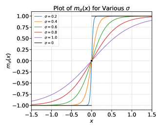
Example 3.5.

Let $p=\frac{1}{2}\delta_{-1}+\frac{1}{2}\delta_{1}$ be a probability measure on $\mathbb{R}^{1}$ . Then, the support $\Omega:=\mathrm{supp}(p)=\{-1,1\}$ is just a two-point set. The medial axis is the singleton $\Sigma_{\Omega}=\{0\}$ whose distance to either point is $1$ . Now, we can explicitly write down the denoiser $m_{\sigma}$ as follows:

m_{\sigma}(x)=\frac{-\exp\left(-\frac{(x+1)^{2}}{2\sigma^{2}}\right)+\exp\left(-\frac{(x-1)^{2}}{2\sigma^{2}}\right)}{\exp\left(-\frac{(x+1)^{2}}{2\sigma^{2}}\right)+\exp\left(-\frac{(x-1)^{2}}{2\sigma^{2}}\right)}.

(12)

Notice that when $\sigma$ approaches $0$ ,

•

The denoiser $m_{\sigma}$ is converging to a function $f:\mathbb{R}^{1}\to\{-1,0,1\}$ with $f(x)=1$ for $x>0$ , $f(x)=-1$ for $x<0$ and $f(0)=0$ .
•

Certain singularity of $m_{\sigma}$ is emerging at $\Sigma_{\Omega}=\{0\}$ : the derivative (Jacobian if in high dimensions) $\frac{dm_{\sigma}(0)}{dx}$ is blowing up when $\sigma\to 0$ .

A full characterization of the limit $\lim_{\sigma\to 0}m_{\sigma}(x)$ for discrete data distribution will be given in Corollary 4.12 where the discontinuity often arises at the medial axis of the data support. All these singularities pose challenges in theoretical analysis of the flow matching ODEs and particularly in the convergence of the ODE trajectory when approaching the terminal time. The data geometry singularity is more challenging to handle, especially the discontinuity behavior of the limit of the denoiser near the medial axis.

We will address these challenges in the convergence analysis of the flow matching ODEs in Section 5 by showing that even if the geometric singularities exist, the ODE trajectory will avoid the singularities and converge to the data support. This is done by identifying an absorbing and attracting property of the ODE dynamics, which will be discussed in the next section.

3.3 Denoiser and ODE dynamics: attracting and absorbing

Assume that the ODE trajectory exists and unique up to the terminal time—on $[0,1)$ for $t$ , and on $(0,\infty)$ (resp. $(-\infty,\infty)$ ) for $\sigma$ (resp. $\lambda$ ). In Section 5.1, we rigorously establish this well-posedness for any data distribution $p$ with finite second moments. The Equation 8 suggests that the sample simply moves towards the denoiser $m_{\sigma}$ from its current position $x_{\sigma}$ . However, the main challenge is that the denoiser $m_{\sigma}$ itself evolves along the trajectory.

Nevertheless, when certain coarse geometric information is available, one can provide preliminary insights into the ODE dynamics. Intuitively, as discussed in the introduction, the flow matching ODE initially points towards the data mean and later towards local clusters. These concepts can be described in terms of distance to certain set. Specifically, the flow matching ODE exhibits two key properties when the denoiser $m_{\sigma}$ meets certain conditions that we will elaborate later.

•

Attracting Property: Trajectories are drawn towards specific closed set, i.e, the distance to the set decreases along the trajectory.
•

Absorbing Property: Trajectories remain confined within neighborhoods of certain closed set.

The closed sets that we work with can be a point (e.g. the data mean or a single training data), a convex set (e.g. certain convex hull of data), or a more general set (e.g. the data support). These properties are formalized in the following two meta-theorems. We describe them with respect to $\sigma$ , but they can be translated to $t$ or $\lambda$ in a straightforward manner.

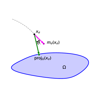
Attracting towards sets.

Let $\Omega$ be a closed set in $\mathbb{R}^{d}$ . We want to examine the distance to $\Omega$ along the ODE trajectory $(x_{\sigma})_{\sigma\in(\sigma_{2},\sigma_{1}]}$ with some $\sigma_{1}>\sigma_{2}$ . Assume that the trajectory avoids the medial axis of $\Omega$ then the distance of $x_{\sigma}$ to $\Omega$ will decrease as $\sigma$ decreases if the trajectory direction $\frac{1}{\sigma}\left(m_{\sigma}(x_{\sigma})-x_{\sigma}\right)$ forms an acute angle with the direction pointing towards $\Omega$ , that is

\langle m_{\sigma}(x_{\sigma})-x_{\sigma},\mathrm{proj}_{\Omega}(x_{\sigma})-x_{\sigma}\rangle>0;

see Figure 5 for an illustration.

Notice that whenever $x_{\sigma}\notin\Omega$ , one has

\langle m_{\sigma}(x_{\sigma})-x_{\sigma},\mathrm{proj}_{\Omega}(x_{\sigma})-x_{\sigma}\rangle=\langle m_{\sigma}(x_{\sigma})-\mathrm{proj}_{\Omega}(x_{\sigma}),\mathrm{proj}_{\Omega}(x_{\sigma})-x_{\sigma}\rangle+\|\mathrm{proj}_{\Omega}(x_{\sigma})-x_{\sigma}\|^{2}.

(13)

Hence, as long as the term $\langle m_{\sigma}(x_{\sigma})-\mathrm{proj}_{\Omega}(x_{\sigma}),\mathrm{proj}_{\Omega}(x_{\sigma})-x_{\sigma}\rangle$ is small enough, one would guarantee that the acute angle condition is satisfied and then the distance to $\Omega$ will decrease along the trajectory. This intuition is formalized in the following theorem.

Theorem 3.6 (Attracting towards sets).

Let $(x_{\sigma})_{\sigma\in(\sigma_{2},\sigma_{1}]}$ be an ODE trajectory of Equation 8 starting from some $x_{\sigma_{1}}$ . Assume that the trajectory avoids the medial axis of a closed $\Omega$ then we have the following results.

1.

If $\langle m_{\sigma}(x_{\sigma})-\mathrm{proj}_{\Omega}(x_{\sigma}),\mathrm{proj}_{\Omega}(x_{\sigma})-x_{\sigma}\rangle\leq\zeta\|x_{\sigma}-\mathrm{proj}_{\Omega}(x_{\sigma})\|^{2}$ for some $0\leq\zeta<1$ along the trajectory, then $d_{\Omega}(x_{\sigma})$ decreases along the trajectory with rate:

$d_{\Omega}(x_{\sigma})\leq\frac{\sigma^{1-\zeta}}{\sigma_{1}^{1-\zeta}}d_{\Omega}(x_{\sigma_{1}}),$

In particular, if $\sigma_{2}=0$ , then $d_{\Omega}(x_{\sigma})$ decreases to zero as $\sigma\to 0$ .
2.

If $\sigma_{2}=0$ and $|\langle m_{\sigma}(x_{\sigma})-\mathrm{proj}_{\Omega}(x_{\sigma}),\mathrm{proj}_{\Omega}(x_{\sigma})-x_{\sigma}\rangle|\leq\phi(\sigma)$ for some function $\phi(\sigma)$ along the trajectory with $\lim_{\sigma\to 0}\phi(\sigma)=0$ , then

$\lim_{\sigma\to 0}d_{\Omega}(x_{\sigma})=0.$

Remark 3.7.

In fact, when considering the parameter $\lambda=-\log(\sigma)$ and the trajectory $z_{\lambda}:=x_{\sigma(\lambda)}$ , we obtain the following convergence rate for Item 2 in the above theorem:

d_{\Omega}(z_{\lambda})\leq e^{-(\lambda-\lambda_{1})}d_{\Omega}(z_{\lambda_{1}})+e^{-\lambda}\sqrt{\int_{\lambda_{1}}^{\lambda}2e^{2t}\phi(t)dt}.

The above theorems require the trajectory to avoid the medial axis of $\Omega$ . We will find two situations that this condition is satisfied: (1) when $\Omega$ is a convex set as its medial axis is empty. It turns out one can identify specific convex sets in different stages of the flow matching ODE dynamics where the denoiser satisfies the above estimates and hence the ODE trajectory is attracted towards these convex sets. We will discuss these in Sections 6.1 and 6.2. (2) when we can show that the trajectory will confined in a region outside the medial axis of $\Omega$ . This is in particular related to the terminal behavior of the flow model sampling process which includes the convergence of the flow matching ODE to the data support which will be discussed in Section 5.2 and Section 6.3. Furthermore, the estimates in the conditions of the above theorem is related with the concentration properties of the posterior distribution $p(\cdot|\bm{X}_{\sigma}=x)$ which we will discuss in Section 4.

We now describe a general absorbing property in the next paragraph.

Absorbing by sets.

Let $\Omega$ be any set in $\mathbb{R}^{d}$ . For any $0\leq\sigma_{2}<\sigma_{1}$ , we say $\Omega$ is absorbing for the flow matching ODE in $(\sigma_{2},\sigma_{1}]$ , if for any $x\in\Omega$ , the ODE trajectory $(x_{\sigma})_{\sigma\in(\sigma_{2},\sigma_{1}]}$ for Equation 8 starting at $x_{\sigma_{1}}=x$ will remain in $\Omega$ for all $\sigma\in(\sigma_{2},\sigma_{1}]$ .

Now, we assume that $\Omega$ is closed. It turns out that the acute angel condition

\langle m_{\sigma}(x)-x,\mathrm{proj}_{\Omega}(x)-x\rangle>0

will also guarantee that the trajectory will remain confined within a neighborhood of $\Omega$ . This is formalized in the following theorem.

Theorem 3.8 (Absorbing by sets).

For any closed set $\Omega$ and $r>0$ , we consider the open neighborhood $B_{r}(\Omega)$ .

1.

If $\overline{B_{r}(\Omega)}\cap\Sigma_{\Omega}=\emptyset$ and for any $x\in\partial B_{r}(\Omega)$ and any $\sigma\in(\sigma_{2},\sigma_{1})$ , one has

$\langle m_{\sigma}(x)-x,\mathrm{proj}_{\Omega}(x)-x\rangle>0,$

then $B_{r}(\Omega)$ is absorbing in $(\sigma_{2},\sigma_{1}]$ .
2.

If there exists some $r_{0}>0$ such that $B_{r}(\Omega)$ is absorbing in $(\sigma_{2},\sigma_{1}]$ for all $r\in(0,r_{0})$ , then $\Omega$ is absorbing in $(\sigma_{2},\sigma_{1}]$ as well.

Note that the absorbing property only requires the denoiser information in some fixed region rather than a priori knowledge of how the denoiser evolves along the trajectory. This versatility makes the absorbing property to be utilized as a first step of controlling the ODE dynamics in many of our analysis.

We now describe how will we use the above absorbing property for convex sets which will be used often in Section 6, and how its generalization will be used to analyze the convergence of the flow matching ODEs in Section 5.2.

For a convex set $K$ , its the medial axis $\Sigma_{K}$ is empty and if we assume that the denoiser $m_{\sigma}$ lies in $K$ for any $x\in\partial B_{r}(K)$ then any neighborhood of $K$ will be absorbing for the ODE trajectory. We also obtain an stronger result regarding when the set $K$ itself is absorbing.

Proposition 3.9 (Absorbing of convex sets).

Let $K$ be a closed convex set in $\mathbb{R}^{d}$ . Let $(x_{\sigma})_{\sigma\in(\sigma_{2},\sigma_{1}]}$ be an ODE trajectory of Equation 8. Then, we have the following results.

1.

For any $r>0$ , if $m_{\sigma}(x)\in K$ for any $x\in\partial B_{r}(K)$ and any $\sigma\in(\sigma_{2},\sigma_{1}]$ , then $B_{r}(K)$ is absorbing for $(x_{\sigma})_{\sigma\in(\sigma_{2},\sigma_{1}]}$ .
2.

If the interior $K^{\circ}$ of $K$ is not empty and $m_{\sigma}(x)\in K^{\circ}$ for any $x\in\partial K$ and any $\sigma\in(\sigma_{2},\sigma_{1}]$ , then $K$ is absorbing for $(x_{\sigma})_{\sigma\in(\sigma_{2},\sigma_{1}]}$ .

Remark 3.10.

When $\Omega$ is not convex, a typical way to show the acute angle condition is by requiring $\|m_{\sigma}(x)-\mathrm{proj}_{\Omega}(x)\|$ to be small enough on $\partial B_{r}(\Omega)$ for all $\sigma\in(\sigma_{2},\sigma_{1}]$ . This can be seen by the following computation:

	$\displaystyle\langle m_{\sigma}(x_{\sigma})-x_{\sigma},\mathrm{proj}_{\Omega}(x_{\sigma})-x_{\sigma}\rangle$	$\displaystyle=\langle m_{\sigma}(x_{\sigma})-\mathrm{proj}_{\Omega}(x_{\sigma}),\mathrm{proj}_{\Omega}(x_{\sigma})-x_{\sigma}\rangle+\\|\mathrm{proj}_{\Omega}(x_{\sigma})-x_{\sigma}\\|^{2}$
		$\displaystyle\geq-\\|m_{\sigma}(x_{\sigma})-\mathrm{proj}_{\Omega}(x_{\sigma})\\|\\|\mathrm{proj}_{\Omega}(x_{\sigma})-x_{\sigma}\\|+\\|\mathrm{proj}_{\Omega}(x_{\sigma})-x_{\sigma}\\|^{2}.$

Furthermore, once the absorbing property is established, it guarantees that $d_{\Omega}(x_{\sigma})=\|\mathrm{proj}_{\Omega}(x_{\sigma})-x_{\sigma}\|$ to be bounded for a trajectory in consideration. In this case, the condition in Item 2 of the attracting theorem Theorem 3.6 can be derived from the decay of $\|m_{\sigma}(x_{\sigma})-\mathrm{proj}_{\Omega}(x_{\sigma})\|$ as

|\langle m_{\sigma}(x_{\sigma})-\mathrm{proj}_{\Omega}(x_{\sigma}),\mathrm{proj}_{\Omega}(x_{\sigma})-x_{\sigma}\rangle|\leq\|m_{\sigma}(x_{\sigma})-\mathrm{proj}_{\Omega}(x_{\sigma})\|\|\mathrm{proj}_{\Omega}(x_{\sigma})-x_{\sigma}\|.

These type of arguments will be utilize in Section 6.2 and Section 6.3 when discussing the ODE dynamics of the flow matching ODEs.

When $\Omega$ is unbounded, e.g the support of a general distribution, it would require much more assumptions for us to control the term $\|m_{\sigma}(x_{\sigma})-\mathrm{proj}_{\Omega}(x_{\sigma})\|$ uniformly on the boundary. As one way to circumvent this issue, we consider the intersection of $B_{r}(\Omega)$ with a bounded set and establish the absorbing property of the bounded subset. This is formalized in the following result.

Theorem 3.11 (Absorbing of data support).

Fix any small $0<\delta<\tau_{\Omega}/4$ and any $0<\zeta<1$ . Assume that there exists a constant $\sigma_{\Omega}>0$ such that for any $R>\frac{1}{2}\tau_{\Omega}$ and for any $z\in B_{R}(0)\cap B_{\tau_{\Omega}/2}(\Omega)$ , one has that

\|m_{\sigma}(z)-\mathrm{proj}_{\Omega}(z)\|\leq C_{\zeta,\tau,R}\cdot\sigma^{\zeta},\text{ for all }0<\sigma<\sigma_{\Omega}.

where $C_{\zeta,\tau,R}$ is a constant depending only on $\zeta$ and $\tau$ and $R$ .

Then, there exists $\sigma_{\delta}\leq\sigma_{\Omega}$ dependent on $\delta,\zeta$ and $C_{\zeta,\tau,R}$ satisfying the following property for any $R>2\delta$ : The trajectory $(x_{\sigma})_{\sigma\in(0,\sigma_{\delta}]}$ starting at any initial point $x_{\sigma_{\delta}}\in B_{R}(0)\cap B_{\delta}(\Omega)$ of the ODE in Equation 8 will be absorbed in a slightly larger space: for any $\sigma\leq\sigma_{\delta}$ : $x_{\sigma}\in B_{2R}(0)\cap B_{2\delta}(\Omega)$ .

Note that this absorbing result is slightly different from Theorem 3.8, where the neighborhood of the data support $\Omega$ must be enlarged from $\delta$ to $2\delta$ (and $R$ to $2R$ ) to guarantee the absorbing property. This subtle difference arises from the additional treatment in the proof to account for the bounded ball $B_{R}(0)$ in the above theorem.

We will then be able to show in Section 5.2 that near the terminal time, an ODE trajectory that starts from a point $x$ near the data support $\Omega$ will never leave a neighborhood of the $\Omega$ , which avoids the geometric singularities (cf. Section 3.2), and will eventually be attracted to the $\Omega$ .

4 Concentration and Convergence of the Posterior Distribution

In the previous section, we established how the properties of denoisers influence the behavior of flow matching ODEs. Since denoisers are defined as expectations of posterior distributions, this section provides a detailed analysis of the concentration and convergence of the posterior distribution for a general data distribution $p$ . Such an analysis not only validates the assumptions on denoisers made in the meta-theorems on attraction (Theorem 3.6) and absorption (Theorem 3.8) but also forms the foundation for the ODE analysis in Section 5 and Section 6. Additionally, we discuss the cases when $p$ is supported either on a low-dimensional manifold or on a discrete set to explore the impact of different data geometries. As a natural consequence of the convergence of the posterior distribution, we also establish the convergence of the denoisers.

4.1 Concentration and convergence of the posterior distribution

Intuitively, for the posterior distribution $p(\cdot|\bm{X}_{t}=x)$ , as $t$ goes to $1$ , the noise level $\beta_{t}$ goes to $0$ and hence the posterior distribution should concentrate around data points near $x$ . We will establish this rigorously utilizing the parameter $\sigma$ .

Initially, the posterior distribution $p(\cdot|\bm{X}_{\sigma}=x)$ for large $\sigma$ is close to the data distribution $p$ and hence the ODE trajectory $x_{\sigma}$ will move towards the mean of the data distribution. The following proposition quantifies the initial stability of the posterior distribution.

Proposition 4.1 (Initial stability of posterior measure).

Let $p$ be a probability measure on $\mathbb{R}^{d}$ with bounded support which is denoted as $\Omega:=\mathrm{supp}(p)$ . Let $x$ be a point and consider the posterior measure $p(\cdot|\bm{X}_{\sigma}=x)$ . We then have the following Wasserstein distance bound:

d_{W,1}(p(\cdot|\bm{X}_{\sigma}=x),p)<\left(\exp\left(\frac{2\|x-\mathbb{E}[\bm{X}]\|\mathrm{diam}(\Omega)}{\sigma^{2}}\right)-1\right)\mathrm{diam}(\Omega).

Note that the bound above will only be meaningful when $\sigma$ is large and will blow up to infinity as $\sigma$ decreases to $0$ . This makes sense as the posterior distribution $p(\cdot|\bm{X}_{\sigma}=x)$ will gradually depart from $p$ and concentrate around the data points near $x$ and eventually converge to the delta distribution located at the nearest data point. The following theorem quantifies the concentration and convergence of the posterior distribution.

Theorem 4.2.

Let $\Omega:=\mathrm{supp}(p)$ . Assume that $p$ has finite 2-moment, i.e., $\mathsf{M}_{2}(p):=\int_{\mathbb{R}^{d}}\|x\|^{2}p(dx)<\infty$ . For all $x\in\mathbb{R}^{d}\backslash\Sigma_{\Omega}$ , we let $x_{\Omega}:=\mathrm{proj}_{\Omega}(x)$ . Then, we have that

\lim_{\sigma\to 0}d_{\mathrm{W},2}\left(p(\cdot|\bm{X}_{\sigma}=x),\delta_{x_{\Omega}}\right)=0.

Remark 4.3.

The proof strategy of Theorem 4.2 is similar to that used in [SBDS24, Theorem 4.1], where the integral under consideration is split into two parts to analyze the concentration. However, it is important to note that our result is more general than that in [SBDS24] in two aspects. First, we do not require the data distribution to be supported on a manifold. Second, we do not require the points to be sufficiently close to the data support.

As a direct consequence of the convergence of the posterior distribution, we have the following convergence of the denoiser.

Corollary 4.4.

Under the same assumptions as in Theorem 4.2, we have that for any $x\in\mathbb{R}^{d}\backslash\Sigma_{\Omega}$ , we have that

\lim_{\sigma\to 0}m_{\sigma}(x)=\mathrm{proj}_{\Omega}(x).

When we turn back to the parameter $t$ , we have the following corollary. The proof turns out to be rather technical instead of being a direct consequence of the above theorem. The main difficulty lies in the scaling $\alpha_{t}$ within the exponential term. This is another example that the parameter $\sigma$ is more convenient for theoretical analysis.

Corollary 4.5.

Let $\Omega:=\mathrm{supp}(p)$ . Assume that $p$ has finite 2-moment. For all $x\in\mathbb{R}^{d}\backslash\Sigma_{\Omega}$ , we let $x_{\Omega}:=\mathrm{proj}_{\Omega}(x)$ . Then, we have that

\lim_{t\to 1}m_{t}(x)=\mathrm{proj}_{\Omega}(x).

Finally, we establish the following convergence rate for the posterior distribution when more assumptions are made on the data distribution $p$ .

Theorem 4.6.

Assume that the reach $\tau=\tau_{\Omega}>0$ is positive. Consider any $x\in\mathbb{R}^{d}$ . We assume that $d_{\Omega}(x)<\frac{1}{2}\tau$ and that there exists $g\geq 0$ such that there exist constants $C,c>0$ so that for any small radius $0<r<c$ , one has $p(B_{r}(x_{\Omega}))\geq Cr^{k}$ . Then, for any $0<\zeta<1$ we have the following convergence rate for any $0<\sigma<c^{1/\zeta}$ :

d_{\mathrm{W},2}\left(p(\cdot|\bm{X}_{\sigma}=x),\delta_{x_{\Omega}}\right)\leq\sqrt{\sigma^{2\zeta}+\frac{10^{k}(2\mathsf{M}_{2}(p)+\|x_{\Omega}\|^{2})\max\{\tau^{k},\sigma^{k\zeta}\}}{C\sigma^{2k\zeta}}\exp\left(-\frac{1}{8}\sigma^{2(\zeta-1)}\right)}\leq C_{\zeta,\tau}\sigma^{\zeta},

where $C_{\zeta,\tau}$ is a constant depending only on $\zeta$ and $\tau_{\Omega}$ .

This convergence rate result plays a central role in the subsequent analysis of the convergence of flow matching ODE trajectories (cf. Theorem 5.3). The assumptions underlying this theorem serve as a primary basis for the assumptions outlined in 1, which are critical for our analysis of ODEs. Consequently, any refinement or improvement of this theorem could potentially enhance the subsequent analysis of ODEs.

4.2 Distinct behaviors for posterior convergence rates under data geometry

In this subsection, we will revisit Theorem 4.2 under different data geometries. In particular, we focus on two cases: (1) $p$ is supported on a low-dimensional manifold $M\subset\mathbb{R}^{d}$ with smooth density with respect to the Hausdorff measure (note that we do not exclude the case when $M=\mathbb{R}^{d}$ ); (2) $p$ is a discrete distribution supported on a finite set.

The first case is motivated by the fact that many real-world data distributions are supported on low-dimensional manifolds. However, in practice, one usually has no access to the manifold $M$ but only to some samples drawn from $p$ . Let $M_{N}=\{x^{(1)},\ldots,x^{(N)}\}$ denote $N$ independent samples drawn from $p$ , and let $p^{N}$ denote the corresponding empirical probability measure. When training the objective function in Section 2.2 with the empirical $p_{1}^{N}$ , one unfortunately will obtain the unique empirical optimal solution $u_{t}^{N}(x)$ with closed form:

\displaystyle u_{t}^{N}(x)

\displaystyle=\frac{\dot{\beta}_{t}}{\beta_{t}}x+\frac{\dot{\alpha}_{t}\beta_{t}-\alpha_{t}\dot{\beta}_{t}}{\beta_{t}}\underbrace{\sum_{i=1}^{N}\frac{\exp\left(-\frac{\|x-\alpha_{t}x^{(i)}\|^{2}}{2\beta_{t}^{2}}\right)x_{i}}{\sum_{j=1}^{N}\exp\left(-\frac{\|x-\alpha_{t}x^{(j)}\|^{2}}{2\beta_{t}^{2}}\right)}}_{m_{t}^{N}(x)}.

(14)

Solving the ODE $\frac{dx_{t}}{dt}=u_{t}^{N}(x_{t})$ with $x_{0}\sim p_{0}$ will almost surely result in $x_{1}\in M_{N}$ . This is an extremely undesired effect as no new samples can be generated from the model. To avoid this issue, we believe certain modification of the training objective must be made. In order to achieve this goal, we first need to theoretically contrast the solution $u_{t}(x)$ with the empirical solution $u_{t}^{N}(x)$ under the manifold hypothesis mentioned above. This is why we focus on the convergence rates of the posterior distribution in these two geometries in this section. We also point out that the comparison of posterior distributions is necessary as one can hardly tell the difference between the empirical solution and the ground truth solution at the level of the overall distributions.

Proposition 4.7.

Assume that $M_{N}$ is a good sample of $M$ such that $d_{\mathrm{W},2}(p^{N},p)=\epsilon$ . Then, for any $t\in[0,1]$ , one has that $d_{\mathrm{W},2}(p_{t},p_{t}^{N})\leq\epsilon$ .

This result follows trivially from the fact that convolution will decrease the Wasserstein distance. We point out that, however, there is no simple way of bounding the difference between the posterior distributions $d_{\mathrm{W},2}\left(p(\cdot|\bm{X}_{t}=x),p^{N}(\cdot|\bm{X}_{t}=x)\right)$ using $d_{\mathrm{W},2}(p^{N},p)$ . See Theorem 4.3 and Remark 4.4 in [MSW19] for some relevant results along this line.

In this section, we first tackle the convergence rates for the posterior distributions and will complete the convergence analysis for ODEs in Section 5.3.

An intuitive observation regarding the convergence rates.

We start with an observation regarding the Jacobian of the denoisers $m_{\sigma}(x)$ and $m_{\sigma}^{N}(x)$ . By Corollary 4.4 we have that $\lim_{\sigma\to 0}m_{\sigma}(x)=\mathrm{proj}_{M}(x)$ and $\lim_{\sigma\to 0}m_{\sigma}^{N}(x)=\mathrm{proj}_{M_{N}}(x)$ . Now, we consider the Jacobians of the two projection maps.

Proposition 4.8.

For almost everywhere $x\in\mathbb{R}^{d}$ , we have that

1.

$\nabla\mathrm{proj}_{M}(x)=\Pi_{T_{x_{M}}M}$ where $x_{M}:=\mathrm{proj}_{M}(x)$ and $\Pi_{T_{x_{M}}M}$ is the orthogonal projection onto the tangent space $T_{x_{M}}M$ ;
2.

$\nabla\mathrm{proj}_{M^{N}}(x)=0$ .

Then, Proposition 3.2 and Proposition 4.8 imply the following results: if we assume that the convergence of $m_{\sigma}$ to $\mathrm{proj}_{M}$ (resp. $m_{\sigma}^{N}$ to $\mathrm{proj}_{M^{N}}$ ) holds up to the 1st order derivatives as $t\to 1$ (this assumption is made for illustrative purposes only and is not rigorously justified here, serving instead to motivate the later results), then one has the following convergence as $\sigma\to 0$ :

•

$\frac{1}{2\sigma^{2}}\iint(z-z^{\prime})(z-z^{\prime})^{T}p(dz|\bm{X}_{\sigma}=x)p(dz^{\prime}|\bm{X}_{\sigma}=x)\to\Pi_{T_{x_{M}}M}$
•

$\frac{1}{2\sigma^{2}}\iint(z-z^{\prime})(z-z^{\prime})^{T}p^{N}(dz|\bm{X}_{\sigma}=x)p^{N}(dz^{\prime}|\bm{X}_{\sigma}=x)\to 0$ .

Note the $1/\sigma^{2}$ term in front of the integrals above. That the limits above exist immediately implies the following rate estimates (otherwise, the $1/\sigma^{2}$ term will result in a blowup behaviour instead of the convergence above):

•

$\iint(z-z^{\prime})(z-z^{\prime})^{T}p(dz|\bm{X}_{\sigma}=x)p(dz^{\prime}|\bm{X}_{\sigma}=x)=O(\sigma^{2})$
•

$\iint(z-z^{\prime})(z-z^{\prime})^{T}p^{N}(dz|\bm{X}_{\sigma}=x)p^{N}(dz^{\prime}|\bm{X}_{\sigma}=x)=o(\sigma^{2})$ .

From this, we see that the convergence rate of the posterior must be significantly different when $p$ is supported on a manifold or on discrete points. The illustrative calculation above suggests that (1) the convergence rate for the manifold case should be $O(\sigma)$ , (2) whereas the discrete case should be $o(\sigma)$ . These can be seen by roughly taking a square root for the integrals above as one can vaguely think of the above integrals as certain squares of the posteriors. Now, we establish our final rigorous results below.

Convergence rates for the manifold case.

We first consider the case when $p$ is supported on a submanifold $M\subset\mathbb{R}^{d}$ . Note that this does not exclude the case when $M=\mathbb{R}^{d}$ . Under some mild conditions, we have the following convergence rate for the posterior distribution.

Theorem 4.9.

Let $M\subset\mathbb{R}^{d}$ be a $m$ dimensional closed submanifold (without self-intersection) with a positive reach $\tau_{M}$ . Assume that $p(dx)=\rho(x)\mathrm{vol}_{M}(dx)$ has a smooth non-vanishing density $\rho:M\to\mathbb{R}$ . For any $x\in\mathbb{R}^{d}$ and $\sigma\in(0,\infty)$ , we let $x_{M}:=\mathrm{proj}_{M}(x)$ . If $x\in\mathbb{R}^{d}$ satisfies that $d_{M}(x)<\frac{1}{2}\tau_{M}$ , then we have that

d_{\mathrm{W},2}(p(\cdot|\bm{X}_{\sigma}=x),\delta_{x_{M}})=\sqrt{m}\sigma+O(\sigma^{2}).

Note that the first-order convergence rate depends solely on the dimension of the submanifold, while higher-order information, such as the second fundamental form, is encapsulated within the big O notation. Specifying these higher-order contributions in detail would be an interesting direction for future work.

As a direct consequence of the convergence of the posterior distribution, we have the following convergence of the denoiser.

Corollary 4.10.

Under the same assumptions as in Theorem 4.9, for any $x\in\mathbb{R}^{d}$ satisfying $d_{M}(x)<\frac{1}{2}\tau_{M}$ , we have that

\|m_{\sigma}(x)-x_{M}\|=O(\sigma).

Convergence rates for the discrete case.

Let the data distribution $p=\sum_{i=1}^{N}a_{i}\,\delta_{x_{i}}$ be a general discrete distribution with $x_{1},\ldots,x_{N}\in\mathbb{R}^{d}$ and $a_{1},\ldots,a_{N}>0$ . We use $\Omega=\{x_{1},\ldots,x_{N}\}$ to denote the support of $p$ . We study the concentration and convergence of the posterior measure $p(\cdot|\bm{X}_{\sigma}=x)$ for each $x\in\mathbb{R}^{d}$ , including those $x$ on $\Sigma_{\Omega}$ , the medial axis of $\Omega$ . To this end, we introduce the following notations.

For each point $x\in\mathbb{R}^{d}$ , we denote the set of distance values from $x$ to each point in $\Omega$ as follows:

\mathrm{DV}_{\Omega}(x):=\{\|x-x_{i}\|:x_{i}\in\Omega\}.

(15)

We use $d_{\Omega}(x;i)$ to denote the $i$ -th smallest distance value in $\mathrm{DV}_{\Omega}(x)$ . A useful geometric notion will be the gap between the squares of the two smallest distances which we denote by

\Delta_{\Omega}(x):=d_{\Omega}^{2}(x;2)-d_{\Omega}^{2}(x;1).

(16)

We further let

\mathrm{NN}_{\Omega}(x):=\mathrm{argmin}_{x_{i}\in\Omega}d_{\Omega}(x,x_{i})=\left\{x_{i}\in\Omega:\|x-x_{i}\|=d_{\Omega}(x;1)=\min_{x_{j}\in\Omega}\|x-x_{j}\|\right\}.

We use the notation $\widehat{p}_{\mathrm{NN}(x)}$ to denote the normalized measure restricted to the points in $\Omega$ that are closest to $x$ :

\widehat{p}_{\mathrm{NN}(x)}:=\frac{1}{\sum_{x_{i}\in\mathrm{NN}_{\Omega}(x)}a_{i}}\sum_{x_{i}\in\mathrm{NN}_{\Omega}(x)}a_{i}\,\delta_{x_{i}}.

(17)

Whenever $x$ is not on $\Sigma_{\Omega}$ , we have $\mathrm{NN}_{\Omega}(x)=\{\mathrm{proj}_{\Omega}(x)\}$ and $\widehat{p}_{\mathrm{NN}(x)}=\delta_{\mathrm{proj}_{\Omega}(x)}$ . With the above notation, we have the following convergence result for the posterior measure $p(\cdot|\bm{X}_{\sigma}=x)$ as $\sigma\to 0$ .

Theorem 4.11.

Let $p=\sum_{i=1}^{N}a_{i}\,\delta_{x_{i}}$ be a discrete distribution. For any $x\in\mathbb{R}^{d}$ , we have the following convergence of the posterior measure $p(\cdot|\bm{X}_{\sigma}=x)$ towards $\widehat{p}_{\mathrm{NN}(x)}$ :

d_{\mathrm{W},2}\left(p(\cdot|\bm{X}_{\sigma}=x),\widehat{p}_{\mathrm{NN}(x)}\right)\leq\mathrm{diam}(\Omega)\sqrt{\frac{1-p(\mathrm{NN}_{\Omega}(x))}{p(\mathrm{NN}_{\Omega}(x))}}\exp\left(-\frac{\Delta_{\Omega}(x)}{4\sigma^{2}}\right).

As a corollary, we have the following convergence of the denoiser.

Corollary 4.12.

Let $p=\sum_{i=1}^{N}a_{i}\,\delta_{x_{i}}$ be a discrete distribution. For any $x\in\mathbb{R}^{d}$ , we have the following convergence of the denoiser $m_{\sigma}(x)$ towards the mean of $\widehat{p}_{\mathrm{NN}(x)}$ :

\|m_{\sigma}(x)-\mathbb{E}(\widehat{p}_{\mathrm{NN}(x)})\|\leq\mathrm{diam}(\Omega)\sqrt{\frac{1-p(\mathrm{NN}_{\Omega}(x))}{p(\mathrm{NN}_{\Omega}(x))}}\exp\left(-\frac{\Delta_{\Omega}(x)}{4\sigma^{2}}\right).

In particular, when $x\notin\Sigma_{\Omega}$ , assume that $x_{i}=\mathrm{proj}_{\Omega}(x)$ we have that

\|m_{\sigma}(x)-x_{i}\|\leq\mathrm{diam}(\Omega)\sqrt{\frac{1-a_{i}}{a_{i}}}\exp\left(-\frac{\Delta_{\Omega}(x)}{4\sigma^{2}}\right).

Compared to the linear convergence rate in Corollary 4.10, the discrete setting exhibits an exponential convergence rate. Interestingly, this significant difference does not lead to any notable variation in the flow map convergence rate described in Theorem 5.4. Nevertheless, this discrepancy remains intriguing and could provide valuable insights into understanding the interplay between memorization and generalization in the future. Later in Section 6.3, we will utilize the above results to analyze memorization behavior.

5 Well-Posedness of Flow Matching ODEs

With the concentration and convergence of the posterior distribution established, we now establish the well-posedness of the flow matching ODEs within the interval $t\in[0,1)$ as well as the convergence property when $t\to 1$ , in a general setting, including when the target data distribution $p$ is not fully supported such as those concentrated on a submanifold. This is the first theoretical guarantee for such cases, addressing gaps in prior works [LHH⁺24, GHJ24] that impose restrictive assumptions excluding manifold-supported data.

5.1 Well-posedness of flow matching ODEs at $t\in[0,1)$

First of all, we establish the existence of the flow map $\Psi_{t}$ for $t\in[0,1)$ , i.e., the uniqueness and existence of the solution of Equation 1 for $t\in[0,1)$ . The following result was stated in the original flow matching paper [LCBH⁺22] under unspecified conditions and later on was proved in [GHJ24] in the case when $p$ satisfies many regularity assumptions such as absolute continuity w.r.t. the Lebesgue measure. In our case, we only require that $p$ has finite 2-moment, which significantly expands the applicability of the flow model.

Theorem 5.1.

As long as $p$ has finite 2-moment, for any initial point $x_{0}\in\mathbb{R}^{d}$ , there exists a unique solution $(x_{t})_{t\in[0,1)}$ for the ODE Equation 1. Furthermore, the corresponding flow map $\Psi_{t}$ is continuous and satisfies that $(\Psi_{t})_{\#}p_{\mathrm{prior}}=p_{t}$ for all $t\in[0,1)$ .

This proof involves carefully analyzing $\mathrm{Cov}[\bm{X}|\bm{X}_{t}=x]$ to establish the locally Lipschitz property of the vector field $u_{t}(x)$ as well as establishing the integrability of the vector field so that we can apply the classic mass concentration result (see [Vil09]).

5.2 Well-posedness of flow matching ODEs at $t=1$

Now, we establish the convergence of flow map $\Psi_{t}$ as $t\to 1$ under mild assumptions and hence rule out the potential risk of divergence which can be a disaster for the flow model as shown in Figure 1(a).

Assumption 1 (Regularity assumptions for the data distribution).

Let $p$ be a probability measure on $\mathbb{R}^{d}$ . We assume that $p$ satisfies the following properties:

1.

$p$ has a finite 2-moment, i.e., $\int_{\mathbb{R}^{d}}\|x\|^{2}p(dx)<\infty$ ;
2.

The support $\Omega:=\mathrm{supp}(p)$ has a positive reach $\tau_{\Omega}>0$ ¹¹1The support $\Omega$ can be the whole space $\mathbb{R}^{d}$ and in this case the reach $\tau=\infty$ .;
3.

There exists $k\geq 0$ and $c>0$ such that for any radius $R>0$ , there exist constants $C_{R}$ so that for any small radius $0\leq r<c$ and any $x\in B_{R}(0)\cap\Omega$ , one has $p(B_{r}(x))\geq C_{R}r^{k}$ for any $x\in\Omega$ .

Many common data distributions satisfy the above assumptions and we list some of them below:

Example 5.2.

1.

Any data distribution fully supported on $\mathbb{R}^{d}$ with finite 2 moment and non-vanishing density, e.g., normal distribution, satisfies all the assumptions with $k=d$ .
2.

Any data distribution supported on a $m$ -dimensional linear subspace with finite 2 moment and non-vanishing density, e.g., projected normal distribution, satisfies all the assumptions with $k=m$ .
3.

Any data distribution supported on a $m$ -dimensional compact submanifold $M$ with positive reach with a non-vanishing density with respect to the volume measure on $M$ satisfies all the assumptions with $k=m$ (cf. Lemma B.8).
4.

Any empirical data distribution with a finite number of samples satisfies all the assumptions with $k=0$ .

Now, we establish the main result of this section below. The major reason that we require the reach $\tau_{\Omega}$ to be positive is to handle the geometric singularity mentioned in Section 3.2 through the absorbing result in Theorem 3.11. In this way, we are able to ensure that an ODE trajectory will stay away from the medial axis and hence avoid the potential singularity issue. We need item 3 in 1 to ensure that at least locally, we can apply the posterior convergence rate result in Theorem 4.6 in a uniform way.

Theorem 5.3.

Let $p$ be a probability measure on $\mathbb{R}^{d}$ satisfying the regularity assumptions in 1. Then,

1.

The limit $\Psi_{1}(x):=\lim_{t\to 1}\Psi_{t}(x)$ exists almost everywhere with respect to the Lebesgue measure.
2.

$\Psi_{1}$ is a measurable map and $(\Psi_{1})_{\#}p_{\mathrm{prior}}=p$ .

Furthermore, we have the following estimate of the convergence rate of the flow map. Recall that $\sigma_{t}:=\beta_{t}/\alpha_{t}$ , then, we have that for any fixed $0<\zeta<1$ ,

\|\Psi_{1}(x)-\Psi_{t}(x)\|=O\left(\sigma_{t}^{{\zeta/2}}\right).

The $\zeta$ in the theorem above is inherited from Theorem 4.6. As such, we chose to retain the original formulation, avoiding the simplification of $\sigma_{t}^{{\zeta/2}}$ to $\sigma_{t}^{{\zeta}}$ , which would have required redefining $\zeta\in(0,1/2)$ .

Notice that the convergence rate is for very general data distribution $p$ . In fact, if we further assume that $p$ is supported on a compact manifold or a discrete set, then the convergence rate can be improved. See Section 5.3 below for more details.

5.3 Refined convergence rates for manifolds and discrete cases

Now, we go back to the manifold hypothesis and give a detailed convergence analysis for the manifold case and the sampling case. Based on the convergence rates we established in Section 4.2, we develop the following ODE convergence result which is a refined version of Theorem 5.3. Unlike the vast difference in posterior convergence and in denoiser convergence, the ODE convergence rates of the manifold case and the discrete case are rather similar. This is a bit surprising but we will explain intuitively why this should be the case at the end.

Theorem 5.4.

When $p$ is supported on a submanifold or a discrete set, we have the following convergence rates for the flow map $\Psi_{t}$ as $t\to 1$ .

•

Let $M$ be a $m$ dimensional closed submanifold (without self-intersection). Assume that $p$ has finite 2-moment, and $p(dx)=\rho(x)\mathrm{vol}_{M}(dx)$ has a smooth nonvanishing density $\rho:M\to\mathbb{R}$ and a positive reach $\tau_{M}$ . We further assume that the second fundamental form $\mathbf{I\!I}$ and its covariant derivative $\nabla\mathbf{I\!I}$ are bounded on $M$ . Then, for almost everywhere $x\in\mathbb{R}^{d}$ , we have that

$\|\Psi_{1}(x)-\Psi_{t}(x)\|=O(\sqrt{\sigma_{t}});$
•

If $p=\sum_{i=1}^{N}a_{i}x_{i}$ denotes a discrete probability measure, then for almost everywhere $x\in\mathbb{R}^{d}$ , we have that

$\|\Psi_{1}(x)-\Psi_{t}(x)\|=O(\sigma_{t}).$

Note that the geometric conditions for manifolds in the theorem are mild. These conditions only guarantee that the submanifold will not have “sharp turns” in the ambient space $\mathbb{R}^{d}$ . For example, it includes the case when $M=\mathbb{R}^{d}$ and $M$ is any low dimensional subspace or any compact submanifold, such as a sphere, torus, etc.

The rate for the discrete case is optimal as shown in the example below.

Example 5.5.

Consider the one point set $M_{1}=\{x_{1}\}$ with $p:=\delta_{x_{1}}$ . Then, when choosing $\alpha_{t}=t$ and $\beta_{t}=1-t$ , one has that starting with any $x_{0}\in\mathbb{R}^{d}$ , its ODE trajectory is given by $(x_{t}=(1-t)x_{0}+tx_{1})_{t\in[0,1)}$ . Therefore, $\|x_{1}-x_{t}\|=(1-t)\|x_{0}-x_{1}\|=\Theta(1-t)=\Theta(\sigma_{t})$ . Hence, the flow map $\Psi_{t}$ has a linear convergence rate.

However, we do not know whether the rate for the manifold case is optimal or not. In fact, we conjecture that the rate can be improved to the linear rate $\sigma_{t}$ for the manifold case as well and hence the ODE convergence rate does not differ between the manifold case and the discrete case. This conjecture is motivated from the fact that the distribution $q_{\sigma}\to p$ with linear rate $O(\sigma)$ (see the proposition below) and hence its associated ODE should intuitively converge with the same rate.

Proposition 5.6.

For any probability measure $p$ with finite 2-moment, we have that

d_{\mathrm{W},2}(q_{\sigma},p)=O(\sigma).

We note that the above proposition is relatively straightforward compared to the posterior convergence established in Theorem 4.2. This provides further evidence (in addition to Proposition 4.7 and the subsequent discussion) for the importance of focusing on analyzing the posterior rather than the entire data distribution.

5.4 Equivariance of the flow maps under data transformations

We have established in Theorem 5.3 the existence of the flow map $\Psi_{1}:\mathbb{R}^{d}\to\mathbb{R}^{d}$ sending directly any sampled point $x_{0}\sim p_{\mathrm{prior}}$ to a point $x_{1}$ following the target data distribution $p$ under 1. In this regard, it is of interest to establish theoretical properties of the flow map. In this subsection, we examine how the flow map $\Psi_{1}$ behaves under certain transformations $T:\mathbb{R}^{d}\to\mathbb{R}^{d}$ of the data distribution $p$ . More precisely, after certain transformation, one obtains a new data distribution $\widetilde{p}:=T_{\#}p$ . We then consider applying the flow model to the new data distribution $\widetilde{p}$ and examine the corresponding flow map. In this paper, we assume that $p$ satisfies 1 and focus on rigid transformations and scaling (which will preserve the assumptions), leaving the investigation of other transformations for future work.

Rigid transformations

Consider the rigid transformation $y={\bm{O}}x+b$ where ${\bm{O}}\in\mathbb{R}^{d\times d}$ is an orthogonal matrix and $b\in\mathbb{R}^{d}$ is any vector. It turns out that if we apply the flow model to such a transformed data distribution $\widetilde{p}$ with the same scheduling functions $\alpha_{t}$ and $\beta_{t}$ , the flow map $\widetilde{\Psi}_{1}$ is also a rigid transformation of the original flow map $\Psi_{1}$ , i.e.,

\widetilde{\Psi}_{1}({\bm{O}}x)={\bm{O}}\Psi_{1}(x)+b

In fact, if we let $\widetilde{m}_{t},\widetilde{u}_{t},\widetilde{\Psi}_{t}$ denote the corresponding denoiser, vector field, and flow map associated with $\widetilde{p}$ , we establish the following result.

Theorem 5.7 (Equivariance under rigid transformations).

For any $x\in\mathbb{R}^{d}$ and $t\in[0,1)$ , if we let $y={\bm{O}}x+\alpha_{t}b$ , then

\widetilde{m}_{t}(y)={\bm{O}}m_{t}(x)+b,\,\,\widetilde{u}_{t}(y)={\bm{O}}u_{t}(x)+\dot{\alpha}_{t}b

where $\dot{\alpha}_{t}$ represents the derivative of $\alpha_{t}$ with respect to $t$ . Then, we have that

\widetilde{\Psi}_{t}({\bm{O}}x)={\bm{O}}\Psi_{t}(x)+\alpha_{t}b,

in particular, by convergence of $\Psi_{t}$ as $t\to 1$ , we have that $\widetilde{\Psi}_{1}({\bm{O}}x)={\bm{O}}\Psi_{1}(x)+b$ .

Scaling

We now consider the effect on the flow map when the data is scaled by a factor $k>0$ , i.e., $y=kx$ . This case is more intricate than the previous two cases, as one needs to change the scheduling functions to obtain the invariance property of the flow map.

Assume that an initial flow model is applied to $p$ with scheduling functions $\alpha_{t}$ and $\beta_{t}$ . Let $s_{t}:[0,1]\to\mathbb{R}$ denote any positive smooth function so that $s_{0}=1$ and $s_{1}=k$ . Then, consider

\bar{\alpha}_{t}:=s_{t}\alpha_{t}/k\,\text{ and }\,\bar{\beta}_{t}:=s_{t}\beta_{t}.

These are still legitimate scheduling functions satisfying $\bar{\alpha}_{0}=\bar{\beta}_{1}=0$ and $\bar{\alpha}_{1}=\bar{\beta}_{0}=1$ . We let $\bar{m}_{t},\bar{u}_{t},\bar{\Psi}_{t}$ denote the corresponding denoiser, vector field, and flow map associated with the flow matching model with the scaled data distribution $k\cdot p$ and the new scheduling functions $\bar{\alpha}_{t}$ and $\bar{\beta}_{t}$ . We establish the following result.

Theorem 5.8 (Equivariance under scaling transformations).

For any $x\in\mathbb{R}^{d}$ and $t\in[0,1)$ , if we let $y=s_{t}x$ , then

\bar{m}_{t}(y)=k\cdot m_{t}(x).

Therefore,

\bar{\Psi}_{t}(x)=s_{t}\cdot\Psi_{t}(x)

and in particular, by convergence of $\bar{\Psi}_{t}$ as $t\to 1$ , we have that $\bar{\Psi}_{1}(x)=k\cdot\Psi_{1}(x)$ .

6 Attraction Dynamics of Flow Matching ODEs

In this section, we utilize the concentration and convergence results of the posterior distribution to analyze the attraction dynamics of the flow matching ODEs.

Following the flow matching ODE, when using $\sigma$ , the ODE trajectory can be simply interpreted as moving towards the denoiser at each time step. Intuitively, denoiser $m_{\sigma}(x)$ initially is close to the data mean and then progressively being close to nearby data points as the ODE trajectory evolves. Eventually, as $\sigma$ goes to zero, the denoisers will converge to the nearest data point almost surely. We will instantiate this intuition and provide rigorous results. We will first analyze the initial stage of the sampling process and then discuss the attraction dynamics towards a local cluster of data points in the intermediate stage. Finally, we will discuss the terminal behavior of the ODE trajectory under the discrete measure along with its connection with memorization.

6.1 Initial stage of the sampling process

We will first work with a data distribution $p$ with bounded support and then later extend to a more general setting where $p$ is a convolution of a bounded support distribution and a Gaussian distribution. We assume the data distribution $p$ has finite $2$ -moment and hence the ODE trajectories of the flow model are well-defined (cf. Section 5.1). We now analyze the initial stage of the sampling process in the flow model.

The initial stage of the sampling process corresponds with $\sigma$ being with a large value $T$ with which the initial sample $x_{\sigma=T}$ is transformed from $x_{t_{\sigma=T}}/\alpha_{t_{\sigma=T}}$ . As $T$ is large, $t_{\sigma=T}$ is close to $0$ , and hence $x_{t_{\sigma=T}}/\alpha_{t_{\sigma=T}}$ has an very large norm. In this case, $x_{\sigma=T}$ is likely outside the support of $p_{b}$ . Therefore, the above corollary describes the initial stage of the sampling process.

Attracting toward data mean

By the initial stability of the posterior distribution, the denoiser will be close to the mean of the data distribution which can be summarized in the following proposition.

Proposition 6.1.

Let $p$ be a probability measure on $\mathbb{R}^{d}$ with finite 2-moment and bounded support $\Omega:=\mathrm{supp}(p)$ . Fix any $\zeta\in(0,1)$ . Then, for any $x_{0}\in\mathbb{R}^{d}$ with initial distance $R_{0}:=\|x_{0}-\mathbb{E}[\bm{X}]\|$ where $\bm{X}\sim p$ , there exists a constant

\sigma_{\mathrm{init}}(\Omega,\zeta,R_{0}):=\sqrt{\frac{2R_{0}\mathrm{diam}(\Omega)}{\log\left(1+\frac{\zeta R_{0}}{\mathrm{diam}(\Omega)}\right)}}

such that for all $\sigma_{1}>\sigma_{\mathrm{init}}(\Omega,\zeta,R_{0})$ , the denoiser $m_{\sigma}(x)$ will be close to the mean of the data distribution $p$ with the following estimate:

\|m_{\sigma}(x)-\mathbb{E}[\bm{X}]\|<\zeta\|x-\mathbb{E}[\bm{X}]\|.

With the above proposition, we can then apply the meta absorbing result in Section 3.3 to show that the ODE trajectory will be absorbed in a ball centered at the mean of the data distribution.

Proposition 6.2.

Under the same assumptions as in Proposition 6.1, the closed neighborhood $\overline{B_{R_{0}}(\mathbb{E}[\bm{X}])}$ is an absorbing set for the ODE trajectory $(x_{\sigma})_{\sigma\in(\sigma_{\mathrm{init}}(\Omega,\zeta,R_{0}),\sigma_{1}]}$ .

The abosorbing property guarantees the trajectory will remain in $B_{R_{0}}(\mathbb{E}[\bm{X}])$ and hence the estimate in Proposition 6.1 holds for the trajectory as well. We can then apply the meta attracting result to show the ODE trajectory moves toward the mean of the data distribution in the initial stage.

Proposition 6.3 (Initial stage: Moving towards the data mean).

With the same assumptions as in Proposition 6.1, the ODE trajectory $(x_{\sigma})_{\sigma\in(\sqrt{\sigma_{\mathrm{init}}(\Omega,\zeta,R_{0})^{2}},\sigma_{1}]}$ starting from $x_{\sigma_{1}}=x_{0}$ will move towards the mean of the data distribution $p$ as shown in the following estimate:

\|x_{\sigma}-\mathbb{E}[\bm{X}]\|<\frac{\sigma^{{1-\zeta}}}{\sigma_{1}^{{1-\zeta}}}\|x_{\sigma_{1}}-\mathbb{E}[\bm{X}]\|,

where $\bm{X}\sim p$ .

Note that an $\zeta$ close to $1$ will make $\sigma_{\mathrm{init}}(\Omega,\zeta,R_{0})$ smaller and hence better convergence of the entire sampling process. However, the decay guarantee will be weaker as $\zeta$ approaches 1.

Attracting and abosorbing to the convex hull of data support

How close the trajectory will be to the mean of the data distribution depends on the initial distance and how fast the posterior distribution concentrates. However, the trajectory will necessarily reach the convex hull of the support of $p$ as $\sigma$ goes to zero as shown in the following proposition which is obtained by applying meta theorems of attracting and absorbing in Section 3.3 to the convex hull of the support of $p$ .

Proposition 6.4.

Given the data distribution $p$ defined above, for any $\sigma_{1}>0$ , let $(x_{\sigma})_{\sigma\in(0,\sigma_{1}]}$ be a flow matching ODE trajectory follows Equation 8. Then we have the following results.

1.

If $x_{\sigma_{1}}\in\mathrm{conv}(\mathrm{supp}(p))$ , then $x_{\sigma}\in\mathrm{conv}(\mathrm{supp}(p))$ for any $\sigma\in(0,\sigma_{1}]$ ;

If $x_{\sigma_{1}}\notin\mathrm{conv}(\mathrm{supp}(p))$ , then $x_{\sigma}$ moves towards $\mathrm{conv}(\mathrm{supp}(p))$ with the following decay guarantee:

d_{\mathrm{conv}(\mathrm{supp}(p))}(x_{\sigma})\leq\frac{\sigma}{\sigma_{1}}d_{\mathrm{conv}(\mathrm{supp}(p))}(x_{\sigma_{1}}),

for any $\sigma\in(0,\sigma_{1}]$ .

The above propositions requires the data distribution to have a bounded support. We now extend the above results to a more general setting where the data distribution is $p=p_{b}\ast\mathcal{N}(0,\delta^{2}I)$ , i.e., a convolution of a bounded support distribution and a Gaussian distribution. This is done by noting that the ODE trajectory with data distribution $p$ can be derived from the ODE trajectory with data distribution $p_{b}$ by a simple transformation.

Lemma 6.5.

Let $p_{b}$ be a distribution and let $p:=p_{b}\ast{\mathcal{N}}(0,\delta^{2}I)$ . Let $(y_{\sigma_{b}})_{\sigma_{b}\in(0,\infty)}$ be an ODE trajectory of Equation 5 with data distribution $p_{b}$ . We define $(x_{\sigma}:=y_{\sigma_{b}=\sqrt{\sigma^{2}+\delta^{2}}})_{\sigma\in(0,\infty)}$ . Then, $(x_{\sigma})$ is an ODE trajectory of Equation 5 with data distribution $p$ .

Corollary 6.6.

Let $p=p_{b}\ast\mathcal{N}(0,\delta^{2}I)$ be a probability measure on $\mathbb{R}^{d}$ with $p_{b}$ having a bounded support which is denoted as $\Omega:=\mathrm{supp}(p_{b})$ . Let $x_{0}$ be a point and denote $\|x_{0}-\mathbb{E}[\bm{X}]\|=R_{0}$ , where $\bm{X}\sim p$ . Let $\zeta$ be a parameter such that $0<\zeta<1$ . Then there exist a constant

\sigma_{\mathrm{init}}(\Omega,\zeta,R_{0}):=\sqrt{\frac{2R_{0}\mathrm{diam}(\Omega)}{\log\left(1+\frac{\zeta R_{0}}{\mathrm{diam}(\Omega)}\right)}}

such that for all $\sigma_{1}>\sqrt{\sigma_{\mathrm{init}}(\Omega,\zeta,R_{0})^{2}+\delta^{2}}$ , a trajectory $(x_{\sigma})_{\sigma\in(\sqrt{\sigma_{\mathrm{init}}(\Omega,\zeta,R_{0})^{2}+\delta^{2}},\sigma_{1}]}$ starting from $x_{\sigma_{1}}=x_{0}$ will move towards the mean of the data distribution $p$ . Additionally, we have the following decay result:

\|x_{\sigma}-\mathbb{E}[\bm{X}]\|<\frac{(\sigma^{2}+\delta^{2})^{\frac{1-\zeta}{2}}}{(\sigma_{1}^{2}+\delta^{2})^{\frac{1-\zeta}{2}}}R_{0}.

Corollary 6.7.

Given the data distribution $p$ defined above, for any $\sigma_{1}>0$ , let $x_{\sigma}$ be an ODE trajectory of Equation 8 from $\sigma=\sigma_{1}$ to $\sigma=0$ . Then, we have that

1.

If $x_{\sigma_{1}}\in\mathrm{conv}(\mathrm{supp}(p_{b}))$ , then $x_{\sigma}\in\mathrm{conv}(\mathrm{supp}(p_{b}))$ for any $\sigma\in(0,\sigma_{1}]$ ;

If $x_{\sigma_{1}}\notin\mathrm{conv}(\mathrm{supp}(p_{b}))$ , then $x_{\sigma}$ moves towards $\mathrm{conv}(\mathrm{supp}(p_{b}))$ with the following decay guarantee:

d_{\mathrm{conv}(\mathrm{supp}(p_{b}))}(x_{\sigma})\leq\frac{\sqrt{\sigma^{2}+\delta^{2}}}{\sqrt{\sigma_{1}^{2}+\delta^{2}}}d_{\mathrm{conv}(\mathrm{supp}(p_{b}))}(x_{\sigma_{1}}),

for any $\sigma\in(0,\sigma_{1}]$ .

6.2 Intermediate stage of the sampling process

Now we have described the flow matching ODE dynamics at initial stage. In this subsection, we shed light on the intermediate stage by showing that the ODE trajectory will be attracted towards the convex hull of local clusters of data under some assumptions.

We start by assuming that the data distribution $p$ contains a “local cluster” or “local mode”. More precisely, we consider the following assumptions.

Assumption 2.

Let $p$ be a probability measure on $\mathbb{R}^{d}$ . We assume that $p$ that has a well separated local cluster $S$ , specifically, we assume that $p$ satisfies the following properties:

1.

$\mathrm{supp}(p)=S\cup(\Omega\backslash S)$ , where $S$ is a closed bounded set with diameter $D:=\mathrm{diam}(S)<\infty$ .
2.

$\Omega\backslash S$ satisfies $d_{\mathrm{conv}(S)}(x)>2D$ for all $x\in\Omega\backslash S$ .

Then, it turns out that for any point $y$ that is close to the convex hull of $S$ , the denoiser $m_{\sigma}(y)$ will be attracted to the convex hull of $S$ as $\sigma$ goes to zero.

Proposition 6.8.

Assume that $p$ satisfies 2. Then, for any $x\in\mathbb{R}^{d}$ such that $d_{\mathrm{conv}(S)}(x)\leq D/2-\epsilon$ , we have that

d_{\mathrm{conv}(S)}(m_{\sigma}(x))\leq\mathrm{diam}(\mathrm{supp}(p))\sqrt{\frac{1-a_{S}}{a_{S}}}\exp\left(-\frac{3D\epsilon}{2\sigma^{2}}\right),

where $a_{S}:=p(S)$ which is positive.

Following the strategy illustrated in Remark 3.10, the above proposition can be used to show that the ODE trajectory will be absorbed in certain neighborhood of the convex hull of $S$ and eventually be attracted to the convex hull of $S$ .

Proposition 6.9.

Assume that $p$ satisfies 2. Let $C^{S}_{\epsilon}=\frac{D/2-\epsilon}{\mathrm{diam}(\mathrm{supp}(p))\sqrt{\frac{1-a_{S}}{a_{S}}}}$ , and define

\displaystyle\sigma_{0}(S,\epsilon):=\begin{cases}\exp\left(-\frac{1}{2}\log\left(-\frac{2}{3D\epsilon}\log\left(C^{S}_{\epsilon}\right)\right)\right),&\text{if }C^{S}_{\epsilon}<1,\\ \infty,&\text{otherwise}.\end{cases}

Then, the set $\overline{B_{D/2-\epsilon}(\mathrm{conv}(S))}$ is an absorbing set for the ODE trajectory $(x_{\sigma})_{\sigma\in(0,\sigma_{1}]}$ with $\sigma_{1}<\sigma_{0}(S,\epsilon)$ . Additionally, an ODE trajectory starting from $x_{\sigma_{1}}\in\overline{B_{D/2-\epsilon}(\mathrm{conv}(S))}$ will converge to the convex hull of $S$ as $\sigma\to 0$ .

Remark 6.10.

A well separated local cluster can be regarded as a local mode of the data distribution. The above proposition give a quantitative measure when the ODE trajectory will be attracted to the local mode.

6.3 Terminal stage of the sampling process and memorization behavior

The local cluster dynamics described in the previous subsection can be manifested in the terminal stage of a discrete data distribution where each data point can eventually be regarded as a local cluster. In this subsection, we will show that the ODE trajectory will be attracted to the nearest data point as $\sigma$ goes to zero and discuss the memorization behavior of the flow model. The results in this subsection complement those in Section 5.3 by specifying a precise range of parameters $\sigma$ for terminal convergence, rather than focusing solely on the convergence rate as in Section 5.3.

We will first introduce some necessary notations and definitions. Throughout this subsection, $p$ denotes a discrete distribution $p=\sum_{i=1}^{n}a_{i}\,\delta_{x_{i}}$ . We let $\Omega=\{x_{1},\ldots,x_{n}\}$ denote its support. The Voronoi diagram of $\Omega$ gives a partition of $\mathbb{R}^{d}$ into regions $V_{i}$ ’s based on the closeness to the data points:

V_{i}:=\{x:\|x-x_{i}\|\leq\|x-x_{j}\|,\ \forall x_{j}\in\Omega\}.

In particular, each $V_{i}$ is a connected closed convex region and the union of all $V_{i}$ ’s covers the whole space $\mathbb{R}^{d}$ . The boundary of the region $V_{i}$ consists of exactly the points on $\Sigma_{\Omega}$ , the medial axis of $\Omega$ . We will also consider a family of regions $V_{i}^{\epsilon}$ that lies inside $V_{i}$ and covers all interior points of $V_{i}$ as $\epsilon$ goes to zero. Specifically, let $0<\epsilon<d_{\Omega}(x_{i})$ be a small positive number, we use $V_{i}^{\epsilon}$ to denote the region

V_{i}^{\epsilon}:=\left\{x:\|x-x_{i}\|^{2}\leq\|x-x_{j}\|^{2}-\epsilon^{2},\ \forall x_{j}\in\Omega,\,j\neq i\right\}.

(18)

Similar to the condition for $V_{i}$ , each $V_{i}^{\epsilon}$ is intersection of finitely many half-spaces and hence is a convex region.

For each $y\in V_{i}^{\epsilon}$ , $x_{i}$ is the unique nearest data point to $y$ and the posterior measure $p(\cdot|x_{\sigma}=y)$ will be fully concentrated at $x_{i}$ as $\sigma$ goes to zero as shown in Theorem 4.11. As a consequence, we can identify a time $\sigma_{0}(V_{i}^{\epsilon})$ as follows such that the ODE trajectory will never leave the region $V_{i}^{\epsilon}$ for $\sigma<\sigma_{0}(V_{i}^{\epsilon})$ . We use $\mathrm{sep}(x_{i})$ to denote the minimum distance from $x_{i}$ to other data points in $\Omega$ and introduce a constant $C^{\Omega}_{i,\epsilon}=\frac{2\,\mathrm{sep}(x_{i})}{\mathrm{sep}^{2}(x_{i})-\epsilon^{2}}\cdot\sqrt{\frac{1-a_{i}}{a_{i}}}\cdot\mathrm{diam}(\Omega)$ that depends on the data support $\Omega$ , specific point $x_{i}$ , and the parameter $\epsilon\in(0,\mathrm{sep}(x_{i})/2)$ . Then the time $\sigma_{0}(V_{i}^{\epsilon})$ is defined as

\sigma_{0}(V_{i}^{\epsilon})=\begin{cases}\infty,&\text{if }C^{\Omega}_{i,\epsilon}\leq 1,\\ \frac{\epsilon}{2}\left(\log(C^{\Omega}_{i,\epsilon})\right)^{-1/2},&\text{if }C^{\Omega}_{i,\epsilon}>1,\end{cases}

We have the following proposition.

Proposition 6.11 (Terminal absorbing behavior under discrete distribution).

Fix an arbitrary $0<\sigma_{1}<\sigma_{0}(V_{i}^{\epsilon})$ . Then, for any $y\in V_{i}^{\epsilon}$ , the ODE trajectory $(x_{\sigma})_{\sigma\in(0,\sigma_{0}]}$ starting from $x_{\sigma_{0}}=y$ will stay inside $V_{i}^{\epsilon}$ , i.e., $x_{\sigma}\in V_{i}^{\epsilon}$ .

With the above propositions, we can show that the ODE trajectory inside $V_{i}^{\epsilon}$ will be attracted to $x_{i}$ as $\sigma$ goes to zero.

Proposition 6.12.

Fix an arbitrary $0<\sigma_{0}<\sigma_{0}(V_{i}^{\epsilon})$ . Then, for any $y\in V_{i}^{\epsilon}$ , the ODE trajectory $(x_{\sigma})_{\sigma\in(0,\sigma_{0}]}$ starting from $x_{\sigma_{0}}=y$ will converge to $x_{i}$ as $\sigma$ goes to zero.

Note that this result is complementary to the discrete part of Theorem 5.4 in the sense that we can identify a fairly explicit time $\sigma_{0}(V_{i}^{\epsilon})$ such that the current nearest data point is what the ODE trajectory will converge to. This is in contrast to the general convergence rate of the flow map as $t\to 1$ in Theorem 5.4.

Discussion on Memorization

The constant $\sigma_{0}(V_{i}^{\epsilon})$ in Proposition 6.12 can be regarded as a time under which a trajectory near the data point $x_{i}$ will eventually converge to $x_{i}$ under the flow matching ODE for the empirical data distribution. In particularly, the empirical optimal solution will only be able to repeat the training data points in the terminal stage of the sampling process—a phenomenon known as memorization. The constant $\sigma_{0}(V_{i}^{\epsilon})$ can then be used as a measure of the memorization time for the empirical optimal solution. When considering the CIFAR-10 dataset and choose $\epsilon=1.0$ , the averaged value of $\sigma_{0}(V_{i}^{\epsilon})$ over all data points is around $0.17$ which covers the last one fourth of the sampling process in the popular sampling schedule used in [KAAL22].

Furthermore, we want to emphasize that the memorization for the flow model is particularly depends on the denoiser near terminal time. In particular, if the denoiser is asymptotically close to the empirical denoiser, the flow model will only memorize the empirical data. This is formalized in the following proposition.

For the following, we will consider a neural network trained denoiser $m_{\sigma}^{\theta}$ and its corresponding ODE trajectory $(x_{\sigma}^{\theta})_{\sigma\in(0,\sigma_{0}]}$ following the flow matching ODE with $m_{\sigma}$ replaced by $m_{\sigma}^{\theta}$ , that is,

\displaystyle\frac{dx^{\theta}_{\sigma}}{d\sigma}

\displaystyle=-\frac{1}{\sigma}\left(m_{\sigma}^{\theta}(x_{\sigma})-x^{\theta}_{\sigma}\right),

(19)

Proposition 6.13 (Memorization of trained denoiser).

Let $p$ denote a discrete probability measure and let $m_{\sigma}$ denote its denoiser. Let $m^{\theta}_{\sigma}:\mathbb{R}^{d}\to\mathbb{R}^{d}$ be any smooth map (which should be regarded as any neural network trained denoiser). Assume that there exists a function $\phi(\sigma)$ such that $\lim_{\sigma\to 0}\phi(\sigma)=0$ and

\|m^{\theta}_{\sigma}(x)-m_{\sigma}(x)\|\leq\phi(\sigma),\text{ for all }x\in\mathbb{R}^{d}.

Then, there exists a parameter $\sigma_{0}(V_{i}^{\epsilon},\phi)>0$ such that for all $\sigma_{0}<\sigma_{0}(V_{i}^{\epsilon},\phi)$ , and for any $y\in V_{i}^{\epsilon}$ , the ODE trajectory $(x_{\sigma}^{\theta})_{\sigma\in(0,\sigma_{0}]}$ for Equation 8 (with $m_{\sigma}$ replaced by $m_{\sigma}^{\theta}$ ) starting from $x_{\sigma_{0}}=y$ will converge to $x_{i}$ as $\sigma\to 0$ .

Note that the above proposition do not necessarily specifying the convergence of $x^{\theta}_{\sigma}$ and can be applied in general. In the case where we do have convergence of $x^{\theta}_{\sigma}$ and the the limit of the denoiser $m_{\sigma}^{\theta}(x^{\theta}_{\sigma})$ , the two limits will coincide. This is formalized in the following proposition.

Proposition 6.14.

Let $m_{\sigma}^{\theta}:\mathbb{R}^{d}\to\mathbb{R}^{d}$ be any smooth map (which should be regarded as any neural network trained denoiser). Assume that the ODE trajectory $(x_{\sigma}^{\theta})_{\sigma\in(0,\sigma_{0}]}$ for Equation 8 has a limit as $\sigma\to 0$ and the limit $\lim_{\sigma\to 0}m_{\sigma}^{\theta}(x_{\sigma}^{\theta})$ also exist. Then, we must have that

\lim_{\sigma\to 0}\|m^{\theta}_{\sigma}(x^{\theta}_{\sigma})-x^{\theta}_{\sigma}\|=0.

This proposition shows that the final output of the flow model is fully determined by the behavior of the denoiser near the terminal time unlike a generic ODE where the near terminal time behavior only partially influence the final output. Therefore, for a flow model to have good generalization ability, it is crucial to ensure that the trained denoiser is diverse near terminal time and covers the entire data distribution—where the empirical optimal solution fails.

7 Discussion

Our study lays a steady theoretical foundation for the flow-matching model, especially in the case when data distribution is supported on a low dimensional manifold. Our analysis of the ODE dynamics, as well as the contrast between the manifold and sampling scenarios, will help shed light on designing better variants of the flow matching model that are memorization-free and with better generalization ability.

In particular, we point out the following two possible future directions. Suppose the submanifold $M$ has intrinsic dimension $k$ . Then, $\text{tr}\nabla_{x}m_{1}\equiv k$ whereas $\text{tr}\nabla_{x}m_{1}^{N}\equiv 0$ (cf. Proposition 4.8). From this perspective, one can already see a huge difference between the empirical solution and the ground truth solution. This motivates us to consider incorporating the Jacobian of the denoiser into the training of the flow matching model to minimize memorization. Our analysis of the attraction region of the flow matching ODE in the discrete case also suggests that one should be careful on training the denoiser near the terminal time to avoid memorization.

Our general convergence result contains a coefficient that depends on the reach of the data support which is not stable under perturbations. However, some of our results can potentially be refined by using local variants of the reach, such as the local feature size, which could yield more robust and stronger theoretical guarantees.

Acknowledgements.

This work is partially supported by NSF grants CCF-2112665, CCF-2217058, CCF-2310411 and CCF-2403452.

References

[AB98] Nina Amenta and Marshall Bern. Surface reconstruction by voronoi filtering. In Proceedings of the fourteenth annual symposium on Computational geometry, pages 39–48, 1998.
[AB06] Stephanie B Alexander and Richard L Bishop. Gauss equation and injectivity radii for subspaces in spaces of curvature bounded above. Geometriae Dedicata, 117:65–84, 2006.
[AL19] Eddie Aamari and Clément Levrard. Nonasymptotic rates for manifold, tangent space and curvature estimation. 2019.
[BBDBM24] Giulio Biroli, Tony Bonnaire, Valentin De Bortoli, and Marc Mézard. Dynamical regimes of diffusion models. Nature Communications, 15(1):9957, 2024.
[BDD23] Joe Benton, George Deligiannidis, and Arnaud Doucet. Error bounds for flow matching methods. arXiv preprint arXiv:2305.16860, 2023.
[BHHS22] Clément Berenfeld, John Harvey, Marc Hoffmann, and Krishnan Shankar. Estimating the reach of a manifold via its convexity defect function. Discrete & Computational Geometry, 67(2):403–438, 2022.
[Bia23] Adam Białożyt. The tangent cone, the dimension and the frontier of the medial axis. Nonlinear Differential Equations and Applications NoDEA, 30(2):27, 2023.
[CHN⁺23] Nicolas Carlini, Jamie Hayes, Milad Nasr, Matthew Jagielski, Vikash Sehwag, Florian Tramer, Borja Balle, Daphne Ippolito, and Eric Wallace. Extracting training data from diffusion models. In 32nd USENIX Security Symposium (USENIX Security 23), pages 5253–5270, 2023.
[CLN23] Bennett Chow, Peng Lu, and Lei Ni. Hamilton’s Ricci flow, volume 77. American Mathematical Society, Science Press, 2023.
[CZW⁺24] Defang Chen, Zhenyu Zhou, Can Wang, Chunhua Shen, and Siwei Lyu. On the trajectory regularity of ode-based diffusion sampling. In Forty-first International Conference on Machine Learning, 2024.
[dM37] MR de Mises. La base géométrique du théoreme de m. mandelbrojt sur les points singuliers d’une fonction analytique. CR Acad. Sci. Paris Sér. I Math, 205:1353–1355, 1937.
[DZ11] Michel C Delfour and J-P Zolésio. Shapes and geometries: metrics, analysis, differential calculus, and optimization. SIAM, 2011.
[Efr11] Bradley Efron. Tweedie’s formula and selection bias. Journal of the American Statistical Association, 106(496):1602–1614, 2011.
[EKB⁺24] Patrick Esser, Sumith Kulal, Andreas Blattmann, Rahim Entezari, Jonas Müller, Harry Saini, Dominik Lorenz Yam Levi, Axel Sauer, Frederic Boesel, Dustin Podell, Tim Dockhorn, Zion English, and Robin Rombach. Scaling rectified flow transformers for high-resolution image synthesis. In Forty-first International Conference on Machine Learning, 2024.
[Fed59] Herbert Federer. Curvature measures. Transactions of the American Mathematical Society, 93(3):418–491, 1959.
[GHJ24] Yuan Gao, Jian Huang, and Yuling Jiao. Gaussian interpolation flows. Journal of Machine Learning Research, 25(253):1–52, 2024.
[GHL90] Sylvestre Gallot, Dominique Hulin, and Jacques Lafontaine. Riemannian geometry, volume 2. Springer, 1990.
[GPAM⁺14] Ian Goodfellow, Jean Pouget-Abadie, Mehdi Mirza, Bing Xu, David Warde-Farley, Sherjil Ozair, Aaron Courville, and Yoshua Bengio. Generative adversarial nets. Advances in neural information processing systems, 27, 2014.
[HJA20] Jonathan Ho, Ajay Jain, and Pieter Abbeel. Denoising diffusion probabilistic models. Advances in neural information processing systems, 33:6840–6851, 2020.
[HW20] Daniel Hug and Wolfgang Weil. Lectures on convex geometry, volume 286. Springer, 2020.
[KAAL22] Tero Karras, Miika Aittala, Timo Aila, and Samuli Laine. Elucidating the design space of diffusion-based generative models. Advances in neural information processing systems, 35:26565–26577, 2022.
[KG24] Diederik Kingma and Ruiqi Gao. Understanding diffusion objectives as the elbo with simple data augmentation. Advances in Neural Information Processing Systems, 36, 2024.
[LC24] Marvin Li and Sitan Chen. Critical windows: non-asymptotic theory for feature emergence in diffusion models. arXiv preprint arXiv:2403.01633, 2024.
[LCBH⁺22] Yaron Lipman, Ricky TQ Chen, Heli Ben-Hamu, Maximilian Nickel, and Matthew Le. Flow matching for generative modeling. In The Eleventh International Conference on Learning Representations, 2022.
[LGL23] Xingchao Liu, Chengyue Gong, and Qiang Liu. Flow straight and fast: Learning to generate and transfer data with rectified flow. In International conference on learning representations (ICLR), 2023.
[LGRH⁺24] Gabriel Loaiza-Ganem, Brendan Leigh Ross, Rasa Hosseinzadeh, Anthony L Caterini, and Jesse C Cresswell. Deep generative models through the lens of the manifold hypothesis: A survey and new connections. arXiv preprint arXiv:2404.02954, 2024.
[LHH⁺24] Yaron Lipman, Marton Havasi, Peter Holderrieth, Neta Shaul, Matt Le, Brian Karrer, Ricky TQ Chen, David Lopez-Paz, Heli Ben-Hamu, and Itai Gat. Flow matching guide and code. arXiv preprint arXiv:2412.06264, 2024.
[LZB⁺22] Cheng Lu, Yuhao Zhou, Fan Bao, Jianfei Chen, Chongxuan Li, and Jun Zhu. Dpm-solver: A fast ODE solver for diffusion probabilistic model sampling in around 10 steps. Advances in Neural Information Processing Systems, 35:5775–5787, 2022.
[MMASC14] Maria G Monera, A Montesinos-Amilibia, and Esther Sanabria-Codesal. The taylor expansion of the exponential map and geometric applications. Revista de la Real Academia de Ciencias Exactas, Fisicas y Naturales. Serie A. Matematicas, 108:881–906, 2014.
[MMWW23] Facundo Mémoli, Axel Munk, Zhengchao Wan, and Christoph Weitkamp. The ultrametric Gromov–Wasserstein distance. Discrete & Computational Geometry, 70(4):1378–1450, 2023.
[MSLE21] Chenlin Meng, Yang Song, Wenzhe Li, and Stefano Ermon. Estimating high order gradients of the data distribution by denoising. Advances in Neural Information Processing Systems, 34:25359–25369, 2021.
[MSW19] Facundo Memoli, Zane Smith, and Zhengchao Wan. The Wasserstein transform. In International Conference on Machine Learning, pages 4496–4504. PMLR, 2019.
[PY24] Frank Permenter and Chenyang Yuan. Interpreting and improving diffusion models from an optimization perspective. In Forty-first International Conference on Machine Learning, 2024.
[RTG98] Yossi Rubner, Carlo Tomasi, and Leonidas J Guibas. A metric for distributions with applications to image databases. In Sixth international conference on computer vision (IEEE Cat. No. 98CH36271), pages 59–66. IEEE, 1998.
[SBDS24] Jan Pawel Stanczuk, Georgios Batzolis, Teo Deveney, and Carola-Bibiane Schönlieb. Diffusion models encode the intrinsic dimension of data manifolds. In Forty-first International Conference on Machine Learning, 2024.
[SDCS23] Yang Song, Prafulla Dhariwal, Mark Chen, and Ilya Sutskever. Consistency models. In International Conference on Machine Learning, pages 32211–32252. PMLR, 2023.
[SDWMG15] Jascha Sohl-Dickstein, Eric Weiss, Niru Maheswaranathan, and Surya Ganguli. Deep unsupervised learning using nonequilibrium thermodynamics. In International conference on machine learning, pages 2256–2265. PMLR, 2015.
[SE19] Yang Song and Stefano Ermon. Generative modeling by estimating gradients of the data distribution. Advances in neural information processing systems, 32, 2019.
[SME21] Jiaming Song, Chenlin Meng, and Stefano Ermon. Denoising diffusion implicit models. In International Conference on Learning Representations, 2021.
[SPC⁺24] Neta Shaul, Juan Perez, Ricky TQ Chen, Ali Thabet, Albert Pumarola, and Yaron Lipman. Bespoke solvers for generative flow models. In The Twelfth International Conference on Learning Representations, 2024.
[Vil03] Cédric Villani. Topics in Optimal Transportation. Number 58. American Mathematical Soc., 2003.
[Vil09] Cédric Villani. Optimal transport: old and new, volume 338. Springer, 2009.
[WLCL24] Yuxin Wen, Yuchen Liu, Chen Chen, and Lingjuan Lyu. Detecting, explaining, and mitigating memorization in diffusion models. In The Twelfth International Conference on Learning Representations, 2024.
[ZYLX24a] Pengze Zhang, Hubery Yin, Chen Li, and Xiaohua Xie. Formulating discrete probability flow through optimal transport. Advances in Neural Information Processing Systems, 36, 2024.
[ZYLX24b] Pengze Zhang, Hubery Yin, Chen Li, and Xiaohua Xie. Tackling the singularities at the endpoints of time intervals in diffusion models. In Proceedings of the IEEE/CVF Conference on Computer Vision and Pattern Recognition, pages 6945–6954, 2024.

Appendix A Geometric Notions and Results

In this section, we recall some basic geometric notions and establish some results that are used in the proofs. The geometric results are of independent interest and can be used in other contexts as well.

A.1 Convex geometry notions and results

In this subsection, we collect some basic notions and results in convex geometry that are used in the proofs. Our main reference is the book [HW20].

We first introduce the definition of a convex set and convex function.

Definition 1 (Convex set).

A set $K\subset\mathbb{R}^{d}$ is called a convex set if for any $x_{1},\ldots,x_{n}\in K$ and $0\leq\alpha_{1},\ldots,\alpha_{n}\leq 1$ such that $\sum_{i=1}^{n}\alpha_{i}=1$ , we have that $\sum_{i=1}^{n}\alpha_{i}x_{i}\in K$ .

Definition 2 (Convex function).

A function $f:\mathbb{R}^{d}\to\mathbb{R}$ is called a convex function if for any $x,y\in\mathbb{R}^{d}$ and $0\leq\alpha\leq 1$ , we have that $f(\alpha x+(1-\alpha)y)\leq\alpha f(x)+(1-\alpha)f(y)$ .

An intermediate result that the sublevel sets $\{f<c\}$ or $\{f\leq c\}$ of a convex function $f$ are convex sets; see [HW20, Remark 2.6].

We now introduce the definition of the convex hull of a set.

Definition 3 (Convex hull [HW20, Definition 1.3, Theorem 1.2]).

The convex hull of a set $\Omega\subset\mathbb{R}^{d}$ is the smallest convex set that contains $\Omega$ and is denoted by $\mathrm{conv}(\Omega)$ . Additionally, we have that

\mathrm{conv}(\Omega)=\left\{\sum_{i=1}^{n}\alpha_{i}x_{i}:k\in\mathbb{N},x_{i}\in\Omega,\alpha_{i}\in[0,1],\sum_{i=1}^{n}\alpha_{i}=1\right\}.

Let $\Omega$ be a set, and $x\in\Omega$ . We say a hyperplane give by a linear function $H$ is a supporting hyperplane of $\Omega$ at $x$ if the following holds:

1.

$H(x)=0$ .
2.

$H(y)\geq 0$ for all $y\in\Omega$ .

For a closed convex set $\Omega$ , every boundary point of $\Omega$ has a supporting hyperplane.

Proposition A.1 (Supporting hyperplane [HW20, Theorem 1.16]).

Let $K$ be a closed convex set in $\mathbb{R}^{d}$ and $x\in\partial K$ . Then, there exists a supporting hyperplane of $K$ at $x$ .

We collect some basic properties regarding the convex set the distance function.

Proposition A.2.

Let $K$ be a convex set in $\mathbb{R}^{d}$ and $\Omega$ be a set in $\mathbb{R}^{d}$ . Then, we have that

1.

For each $x\in\mathbb{R}^{d}$ , there exists a unique point $\mathrm{proj}_{K}(x)\in K$ such that $\|x-\mathrm{proj}_{K}(x)\|=d_{K}(x)$ .
2.

The distance function $d_{K}(x)$ is a convex function.
3.

The thickening of $K$ by a distance $r$ is a convex set, that is $B_{r}(K):=\{x\in\mathbb{R}^{d}:d_{K}(x)\leq r\}$ is a convex set.
4.

The diameter of $\Omega$ is the same as the diameter of its convex hull, that is $\mathrm{diam}(\Omega)=\mathrm{diam}(\mathrm{conv}(\Omega))$ .
5.

Let $a>0$ , then a set $\Omega$ is convex if and only if $a\cdot\Omega$ is convex.

A.2 Metric geometry notions and results

Let $\Omega\subset\mathbb{R}^{d}$ be a closed subset and $\Sigma_{\Omega}$ be the medial axis of $\Omega$ . We let $d_{\Omega}:\mathbb{R}^{d}\to\mathbb{R}$ by defined by $d_{\Omega}(x):=\inf_{y\in\Omega}\|x-y\|$ . In this section, we consider certain properties of the projection function $\mathrm{proj}_{\Omega}:\Sigma_{\Omega}^{c}\to\Omega$ .

We first recall the definition of the local feature size in [AB98] with a slight generalization that we consider all points in $\mathbb{R}^{d}$ instead of only points in $\Omega$ .

Definition 4 ([AB98]).

For any $x\in\mathbb{R}^{d}$ , we define the local feature size $\mathrm{lfs}(x)$ of $x$ as the distance from $x$ to the medial axis of $\Omega$ .

Let $x$ be a point in $\mathbb{R}^{d}$ such that it has a unique projection to $\Omega$ , denoted by $x_{\Omega}:=\mathrm{proj}_{\Omega}(x)$ . We first consider the following set for any $x\in\Sigma_{\Omega}^{c}$ :

T_{\Omega}(x):=\left\{t\geq 0:\mathrm{proj}_{\Omega}\left(x_{\Omega}+t\frac{x-x_{\Omega}}{\|x-x_{\Omega}\|}\right)=x_{\Omega}.\right\}.

Lemma A.3.

we have the following characterizations of $T_{\Omega}(x)$ .

•

$T_{\Omega}(x)$ is an interval.
•

For any $t\in T_{\Omega}(x)$ , we have that $x_{\Omega}+t\frac{x-x_{\Omega}}{\|x-x_{\Omega}\|}\notin{\Sigma_{\Omega}}$ .
•

We let $R_{\Omega}(x):=\sup T_{\Omega}(x)$ . If $0<R_{\Omega}(x)<\infty$ , we have that $x_{\Omega}+R_{\Omega}(x)\frac{x-x_{\Omega}}{\|x-x_{\Omega}\|}\in\overline{\Sigma_{\Omega}}$ .
•

$[0,d_{\Omega}(x)+\mathrm{lfs}(x))\subset T_{\Omega}(x)$ .

Proof of Lemma A.3.

The first three items follow from the pioneering work [Fed59, Theorem 4.8]; see also [DZ11, Theorem 6.2] for more details. We provide a proof for the last item. For the last item, first of all, it is straightforward to see that $[0,d_{\Omega}(x)]\subset T_{\Omega}(x)$ . Now, we assume that $r:=R_{\Omega}(x)\in[d_{\Omega}(x),d_{\Omega}(x)+\mathrm{lfs}(x)).$ This implies that

x_{\Omega}+r\frac{x-x_{\Omega}}{\|x-x_{\Omega}\|}=x+(r-d_{\Omega}(x))\frac{x-x_{\Omega}}{\|x-x_{\Omega}\|}\in\overline{\Sigma_{\Omega}}

and hence

\mathrm{lfs}(x)=d_{\Sigma_{\Omega}}(x)=d_{\overline{\Sigma_{\Omega}}}(x)\leq r-d_{\Omega}(x)<\mathrm{lfs}(x).

This is a contradiction and hence $R_{\Omega}(x)\geq d_{\Omega}(x)+\mathrm{lfs}(x)$ . This concludes the proof. ∎

Next, for any point $b\in\Omega$ , we analyze the angle $\angle xx_{\Omega}b$ for any $b\in\Omega$ . The following lemma is a slight variant of [Fed59, Theorem 4.8 (7)].

Lemma A.4.

For any $x\in\Sigma_{\Omega}^{c}$ and any $t>0$ such that $t\in T_{\Omega}(x)$ , the following holds for any $b\in\Omega$ :

\left\langle x-x_{\Omega},x_{\Omega}-b\right\rangle\geq-\frac{\|x_{\Omega}-b\|^{2}\|x-x_{\Omega}\|}{2t}

Proof.

By definition of $T_{\Omega}(x)$ , we have that $\mathrm{proj}_{\Omega}\left(x_{\Omega}+t\frac{x-x_{\Omega}}{\|x-x_{\Omega}\|}\right)=x_{\Omega}$ . Therefore, we have that

	$\displaystyle\left\\|x_{\Omega}+t\frac{x-x_{\Omega}}{\\|x-x_{\Omega}\\|}-b\right\\|^{2}$	$\displaystyle\geq d_{\Omega}^{2}\left(x_{\Omega}+t\frac{x-x_{\Omega}}{\\|x-x_{\Omega}\\|}\right)=t^{2}$
	$\displaystyle\\|x_{\Omega}-b\\|^{2}+2t\left\langle x_{\Omega}-b,\frac{x-x_{\Omega}}{\\|x-x_{\Omega}\\|}\right\rangle+t^{2}$	$\displaystyle\geq t^{2}$
	$\displaystyle 2t\left\langle x_{\Omega}-b,x-x_{\Omega}\right\rangle$	$\displaystyle\geq-\\|x_{\Omega}-b\\|^{2}\\|x-x_{\Omega}\\|$
	$\displaystyle\left\langle x-x_{\Omega},x_{\Omega}-b\right\rangle$	$\displaystyle\geq-\frac{\\|x_{\Omega}-b\\|^{2}\\|x-x_{\Omega}\\|}{2t}$

∎

When $\Omega$ is convex, then $T_{\Omega}(x)=[0,\infty)$ . In this way, we have the following corollary.

Corollary A.5.

If $\Omega$ is convex, then for any $b\in\Omega$ and any $x\in\mathbb{R}^{d}$ we have that $\langle x-x_{\Omega},x_{\Omega}-b\rangle\geq 0$ .

This control of the angle $\angle xx_{\Omega}b$ allows us to derive the following result that bounds the distance between $b\in\Omega$ and the projection $\mathrm{proj}_{\Omega}(x)$ in terms of the distance between $b$ and $x$ .

Lemma A.6.

For any $x\in\Sigma_{\Omega}^{c}$ and any $t>0$ such that $t\in T_{\Omega}(x)$ , we have that for any $b\in\Omega$ ,

\|x-b\|^{2}\geq d_{\Omega}(x)^{2}+\|b-x_{\Omega}\|^{2}\left(1-\frac{d_{\Omega}(x)}{t}\right).

Proof.

The case when $x\in\Omega$ trivially holds. Below we consider the case when $x\in\Sigma_{\Omega}^{c}\cap\Omega^{c}$ . In this case, $d_{\Omega}(x)>0$ as $\Omega$ is a closed set.

By the law of cosines, we have that

\cos(\angle xx_{\Omega}b)=\frac{d_{\Omega}(x)^{2}+\|b-x_{\Omega}\|^{2}-\|x-b\|^{2}}{2d_{\Omega}(x)\|b-x_{\Omega}\|}

Suppose $\|x-b\|^{2}<d_{\Omega}(x)^{2}+\|b-x_{\Omega}\|^{2}(1-\frac{d_{\Omega}(x)}{t})$ , then we have that

	$\displaystyle\cos(\angle xx_{\Omega}b)$	$\displaystyle=\frac{d_{\Omega}(x)^{2}+\\|b-x_{\Omega}\\|^{2}-\\|x-b\\|^{2}}{2d_{\Omega}(x)\\|b-x_{\Omega}\\|}$
		$\displaystyle>\frac{\\|d_{\Omega}(x)^{2}+\\|b-x_{\Omega}\\|^{2}-d_{\Omega}(x)^{2}-\\|b-x_{\Omega}\\|^{2}+\\|b-x_{\Omega}\\|^{2}\frac{d_{\Omega}(x)}{t}}{2d_{\Omega}(x)\\|b-x_{\Omega}\\|}$
		$\displaystyle=\frac{\\|b-x_{\Omega}\\|^{2}}{2t}.$

By applying Lemma A.4 to $b$ and $x$ , we have that

\left\langle x-x_{\Omega},x_{\Omega}-b\right\rangle\geq-\frac{\|x_{\Omega}-b\|^{2}\|x-x_{\Omega}\|}{2t}.

This implies the following estimate for the cosine of the angle $\angle xx_{\Omega}b$ :

\cos(\angle xx_{\Omega}b)=\frac{\left\langle x-x_{\Omega},b-x_{\Omega}\right\rangle}{\|x-x_{\Omega}\|\|b-x_{\Omega}\|}\leq\frac{\|x_{\Omega}-b\|^{2}}{2t}.

This contradicts the inequality above and hence we must have that

\|x-b\|^{2}\geq d_{\Omega}(x)^{2}+\|b-x_{\Omega}\|^{2}\left(1-\frac{d_{\Omega}(x)}{t}\right).

We then have the following corollary which will be used in the proof of Theorem 4.2.

Corollary A.7.

Fix any $x\in\Sigma_{\Omega}^{c}$ , any $t\in[d_{\Omega}(x),d_{\Omega}(x)+\mathrm{lfs}(x))$ and any $\epsilon>0$ . Then, we have that

B_{\sqrt{d_{\Omega}(x)^{2}+\epsilon^{2}\left(1-d_{\Omega}(x)/t\right)}}\left(x\right)\cap\Omega\subseteq B_{\epsilon}(x_{\Omega})\cap\Omega

Proof.

For any $b\in B_{\sqrt{d_{\Omega}(x)^{2}+\epsilon^{2}\left(1-d_{\Omega}(x)/t\right)}}\left(x\right)\cap\Omega$ , we have that

\|x-b\|^{2}<d_{\Omega}(x)^{2}+\epsilon^{2}\left(1-\frac{d_{\Omega}(x)}{t}\right).

By Lemma A.6, we have that

\|x-b\|^{2}\geq d_{\Omega}(x)^{2}+\|b-x_{\Omega}\|^{2}\left(1-\frac{d_{\Omega}(x)}{t}\right).

Combining the two inequalities, we have that $\|b-x_{\Omega}\|^{2}<\epsilon^{2}$ and hence $b\in B_{\epsilon}(x_{\Omega})\cap\Omega$ . ∎

Finally, we derive the local Lipschitz continuity of the projection function.

Lemma A.8 (Local Lipschitz continuity of the projection).

For any $\epsilon>0$ and for any $x,y\in\mathbb{R}^{d}$ such that $\mathrm{lfs}(x)>\epsilon$ and $\mathrm{lfs}(y)>\epsilon$ , we have that

\|x_{\Omega}-y_{\Omega}\|\leq\left(\frac{\max\{d_{\Omega}(x),d_{\Omega}(y)\}}{\epsilon}+1\right)\|x-y\|.

Proof.

Since $\mathrm{lfs}(x)>\epsilon$ and $\mathrm{lfs}(y)>\epsilon$ , by Lemma A.3 we have that

\mathrm{proj}_{\Omega}\left(x_{\Omega}+(\epsilon+d_{\Omega}(x))\frac{x-x_{\Omega}}{\|x-x_{\Omega}\|}\right)=x_{\Omega}

and

\mathrm{proj}_{\Omega}\left(y_{\Omega}+(\epsilon+d_{\Omega}(y))\frac{y-y_{\Omega}}{\|y-y_{\Omega}\|}\right)=y_{\Omega}.

By applying Lemma A.4 to $x,x_{\Omega},y_{\Omega}$ and separately to $y,y_{\Omega},x_{\Omega}$ , we have that

	$\displaystyle\left\langle x_{\Omega}-y_{\Omega},x-x_{\Omega}\right\rangle$	$\displaystyle\geq-\frac{\\|x_{\Omega}-y_{\Omega}\\|^{2}}{2\left(\epsilon+d_{\Omega}(x)\right)}d_{\Omega}(x)$
	$\displaystyle\left\langle y_{\Omega}-x_{\Omega},y-y_{\Omega}\right\rangle$	$\displaystyle\geq-\frac{\\|x_{\Omega}-y_{\Omega}\\|^{2}}{2\left(\epsilon+d_{\Omega}(y)\right)}d_{\Omega}(y)$

By adding the two inequalities about the inner products, we have that

	$\displaystyle\left\langle x_{\Omega}-y_{\Omega},x-x_{\Omega}-y+y_{\Omega}\right\rangle$	$\displaystyle\geq-\frac{\\|x_{\Omega}-y_{\Omega}\\|^{2}}{2\left(\epsilon+d_{\Omega}(x)\right)}d_{\Omega}(x)-\frac{\\|x_{\Omega}-y_{\Omega}\\|^{2}}{2\left(\epsilon+d_{\Omega}(y)\right)}d_{\Omega}(y)$
	$\displaystyle\left\langle x_{\Omega}-y_{\Omega},x-y\right\rangle-\\|x_{\Omega}-y_{\Omega}\\|^{2}$	$\displaystyle\geq-\frac{\\|x_{\Omega}-y_{\Omega}\\|^{2}}{2\left(\epsilon+d_{\Omega}(x)\right)}d_{\Omega}(x)-\frac{\\|x_{\Omega}-y_{\Omega}\\|^{2}}{2\left(\epsilon+d_{\Omega}(y)\right)}d_{\Omega}(y)$
	$\displaystyle\left\langle x_{\Omega}-y_{\Omega},x-y\right\rangle$	$\displaystyle\geq\\|x_{\Omega}-y_{\Omega}\\|^{2}-\frac{\\|x_{\Omega}-y_{\Omega}\\|^{2}}{2\left(\epsilon+d_{\Omega}(x)\right)}d_{\Omega}(x)-\frac{\\|x_{\Omega}-y_{\Omega}\\|^{2}}{2\left(\epsilon+d_{\Omega}(y)\right)}d_{\Omega}(y)$

Let $m=\max\{d_{\Omega}(x),d_{\Omega}(y)\}$ , then we have that

0<1-\frac{m}{m+\epsilon}\leq\left(1-\frac{d_{\Omega}(x)}{2\left(\epsilon+d_{\Omega}(x)\right)}-\frac{d_{\Omega}(y)}{2\left(\epsilon+d_{\Omega}(y)\right)}\right)

Therefore, by Cauchy-Schwarz inequality, we have that

\|x_{\Omega}-y_{\Omega}\|^{2}\left(1-\frac{m}{m+\epsilon}\right)\leq\left\langle x_{\Omega}-y_{\Omega},x-y\right\rangle\leq\|x_{\Omega}-y_{\Omega}\|\|x-y\|

This implies $\|x_{\Omega}-y_{\Omega}\|\leq\left(\frac{m+\epsilon}{\epsilon}\right)\|x-y\|$ . ∎

Differentiability of the distance function

Let $\Omega\subset\mathbb{R}^{d}$ be any closed subset. We let $\Sigma(x):=\{y\in\Omega:\|x-y\|=d_{\Omega}(x)\}$ denote the set of points in $\Omega$ that achieve the infimum. When $x$ is not in the medial axis of $\Omega$ , the set $\Sigma(x)$ is a singleton and we denote it by $\mathrm{proj}_{\Omega}(x)$ .

Interestingly, there is the following result result showing the existence of one sided directional derivatives for $d_{\Omega}$ by [dM37] (see also [Bia23] for a more recent English treatment).

Lemma A.9 ([dM37]).

For any vector $v\in\mathbb{R}^{d}$ , the one-sided directional derivative of $d_{\Omega}$ at $x\in\mathbb{R}^{d}\backslash\Omega$ in the direction $v$ exists and is given by

D_{v}d_{\Omega}(x)=\inf\left\{-\frac{\langle v,y-x\rangle}{\|y-x\|}:y\in\Sigma(x)\right\}

Motivated by the this result, we mimick the proof and establish the following result for the squared distance function $d_{\Omega}^{2}$ . Notice that, we can remove the constraint for $x\notin\Omega$ .

Lemma A.10.

For any $x\in\mathbb{R}^{d}\backslash\Sigma_{\Omega}$ , the directional derivative of $d_{\Omega}^{2}$ at $x$ exists and is given by

D_{v}d_{\Omega}^{2}(x)=-2\langle v,\mathrm{proj}_{\Omega}(x)-x\rangle

Proof.

Without loss of generality, we assume that $x=0$ is the origin and $v=(c,0,\ldots,0)$ for some $c>0$ (one can achieve these by applying rigid transformations).

We let $x_{\Omega}=\mathrm{proj}_{\Omega}(x)$ , $x_{t}=tv$ and $x_{t}^{*}=\mathrm{proj}_{\Omega}(x_{t})$ . Since $\|x_{t}^{*}-x_{t}\|\leq\|x_{\Omega}-x_{t}\|$ , we have that

\|x_{t}^{*}\|^{2}-\|x_{\Omega}\|^{2}\leq 2ct(x_{t}^{*,(1)}-x_{0}^{*,(1)}),

where $x_{t}^{*,(1)}$ denotes the first coordinate of $x_{t}^{*}$ . Note that $\|x_{t}^{*}\|=\|x_{t}^{*}-x\|\geq\|x_{\Omega}-x\|=\|x_{\Omega}\|$ . So we have that

0\leq x_{t}^{*,(1)}-x_{0}^{*,(1)}.

Now we have that by the cosine rule of the triangle formed by $x_{t}=tv$ , $x=0$ and $x_{t}^{*}$ , we have that

d^{2}_{\Omega}(x_{t})=\|x_{t}^{*}\|^{2}+t^{2}c^{2}-2t\langle v,x_{t}^{*}-x\rangle.

Therefore, we have that

\displaystyle\frac{d_{\Omega}^{2}(x_{t})-d_{\Omega}^{2}(x)}{t}=\frac{\|x_{t}^{*}\|^{2}-\|x_{\Omega}\|^{2}}{t}-2\langle v,x_{t}^{*}-x\rangle

As discussed above, we have that

0\leq\frac{\|x_{t}^{*}\|^{2}-\|x_{\Omega}\|^{2}}{t}\leq 2c(x_{t}^{*,(1)}-x_{0}^{*,(1)})

By continuity of $\mathrm{proj}_{\Omega}$ outside $\Sigma_{\Omega}$ , we have that $x_{t}^{*}\to x^{*}$ as $t\to 0$ . Therefore, we have that

\lim_{t\to 0}\frac{d_{\Omega}^{2}(x_{t})-d_{\Omega}^{2}(x)}{t}=-2\langle v,x^{*}-x\rangle=-2\langle v,\mathrm{proj}_{\Omega}(x)-x\rangle.

Corollary A.11.

Let $(x_{t})_{t}$ be a differentiable curve in $x\in\mathbb{R}^{d}\backslash\Sigma_{\Omega}$ , then we have that $d_{\Omega}^{2}(x_{t})$ is differentiable with respect to $t$ and we have that

\frac{d}{dt}d_{\Omega}^{2}(x_{t})=D_{\dot{x}_{t}}d_{\Omega}^{2}(x_{t})=-2\langle\dot{x}_{t},\mathrm{proj}_{\Omega}(x_{t})-x_{t}\rangle

Appendix B Proofs

B.1 Proofs in Section 2

Proof of Proposition 2.1.

For any $x\in\mathbb{R}^{d}$ and $t\in(0,1]$ , $\alpha_{t}>0$ and the map $F_{t}$ is well-defined.

$\displaystyle(F_{t})_{\#}p_{t}$	$\displaystyle=(F_{t})_{\#}\left(\int{\mathcal{N}}(\cdot\|\alpha_{t}x_{0},\beta_{t}^{2}I)p(dx_{0})\right)$
	$\displaystyle=\int{\mathcal{N}}(\cdot\|x_{0},(\beta_{t}/\alpha_{t})^{2}I)p(dx_{0})$
	$\displaystyle=\int{\mathcal{N}}(\cdot\|x_{0},\sigma_{t}^{2}I)p(dx_{0}).$	∎

Proof of Proposition 2.2.

We first write down the density of $q_{\sigma}$ explicitly as follows:

q_{\sigma}(x)=\frac{1}{{(2\pi\sigma^{2})^{d/2}}}\int\exp\left(-\frac{\|x-x_{1}\|^{2}}{2\sigma^{2}}\right)p(dx).

Then, we have that

\nabla\log q_{\sigma}(x)=-\frac{1}{\sigma^{2}}\left(x-\frac{\int y\exp\left(-\frac{\|x-y\|^{2}}{2\sigma^{2}}\right)p(dy)}{\int\exp\left(-\frac{\|x-y^{\prime}\|^{2}}{2\sigma^{2}}\right)p(dy^{\prime})}\right).

Note that $\frac{dt}{d\sigma}=\frac{\alpha_{t}^{2}}{\dot{\beta}_{t}\alpha_{t}-\beta_{t}\dot{\alpha}_{t}}$ . Therefore with the reparametrization ${x}_{\sigma}:=x_{t}/\alpha_{t}$ , we have that

$\displaystyle\frac{dx_{\sigma}}{d\sigma}$	$\displaystyle=\frac{dx_{\sigma}}{dt}\frac{dt}{d\sigma}=\frac{1}{\alpha_{t}^{2}}\left(\alpha_{t}\frac{dx_{t}}{dt}-\dot{\alpha}_{t}x_{t}\right)\frac{dt}{d\sigma}$
	$\displaystyle=\frac{\alpha_{t}}{\beta_{t}}\left(\frac{x_{t}}{\alpha_{t}}-\int\frac{\exp\left(-\frac{\\|x_{t}-\alpha_{t}y\\|^{2}}{2\beta_{t}^{2}}\right)y}{\int\exp\left(-\frac{\\|x_{t}-\alpha_{t}y^{\prime}\\|^{2}}{2\beta_{t}^{2}}\right)p(dy^{\prime})}p(dy)\right)$
	$\displaystyle=-{\sigma}\nabla\log q_{\sigma}(x_{\sigma}).$	∎

B.2 Proofs in Section 3

Proof of Remark 3.1.

For the normalizing factor $Z=\int\exp\left(-\frac{\|x-\alpha_{t}y^{\prime}\|^{2}}{2\beta_{t}^{2}}\right)p(dy^{\prime})$ , we note that $0<\exp\left(-\frac{\|x-\alpha_{t}y^{\prime}\|^{2}}{2\beta_{t}^{2}}\right)\leq 1$ . Hence, the factor $Z$ must be positive and bounded.

Now, we consider the following integral

\displaystyle\int{\exp\left(-\frac{\|x-\alpha_{t}y\|^{2}}{2\beta_{t}^{2}}\right)\|y\|}p(dy)\leq\int\|y\|p(dy)<\infty.

The last inequality follows from the fact that $p$ has a finite 1-moment. Hence, the posterior distribution $p(\cdot|\bm{X}_{t}=x)$ has a finite 1-moment and the denoiser $m_{t}$ is well-defined. ∎

Proof of Equation 10.

Since $\lambda=-\log\sigma$ , we have that

\frac{d\lambda}{d\sigma}=-\frac{1}{\sigma}

and thus the ODE equation Equation 8 becomes

	$\displaystyle\frac{d{x}_{\lambda}}{d\lambda}$	$\displaystyle=\frac{d{x}_{\sigma(\lambda)}}{d\sigma}\frac{d\sigma}{d\lambda}=-\sigma\nabla\log q_{\sigma}(x_{\sigma})\cdot\left(-{\sigma}\right)$
		$\displaystyle=-x_{\sigma}+\frac{\int y\exp\left(-\frac{\\|x_{\sigma}-y\\|^{2}}{2\sigma^{2}}\right)p(dy)}{\int\exp\left(-\frac{\\|x_{\sigma}-y^{\prime}\\|^{2}}{2\sigma^{2}}\right)p(dy^{\prime})}=m_{\lambda}(x_{\lambda})-x_{\lambda}.$		∎

Proof of Proposition 3.2.

Recall that

m_{t}(x)=\frac{\int\exp\left(-\frac{\|x-\alpha_{t}z\|^{2}}{2\beta_{t}^{2}}\right)z\,p(dz)}{\int\exp\left(-\frac{\|x-\alpha_{t}z\|^{2}}{2\beta_{t}^{2}}\right)\,p(dz)}\text{ and }p(dz|\bm{X}_{t}=x)=\frac{\exp\left(-\frac{\|x-\alpha_{t}z\|^{2}}{2\beta_{t}^{2}}\right)p(dz)}{\int\exp\left(-\frac{\|x-\alpha_{t}z\|^{2}}{2\beta_{t}^{2}}\right)\,p(dz)}.

We let $w_{t}(x,z):=\exp\left(-\frac{\|x-\alpha_{t}z\|^{2}}{2\beta_{t}^{2}}\right)$ . Then,

	$\displaystyle\nabla_{x}m_{t}(x)=$	$\displaystyle\int z\nabla_{x}\left(\frac{\exp\left(-\frac{\\|x-\alpha_{t}z\\|^{2}}{2\beta_{t}^{2}}\right)}{\int\exp\left(-\frac{\\|x-\alpha_{t}z^{\prime}\\|^{2}}{2\beta_{t}^{2}}\right)p(dz^{\prime})}\right)p(dz)$
		$\displaystyle=\left(\int w_{t}(x,z^{\prime})p(dz^{\prime})\right)^{-2}\int z\left(w_{t}(x,z)\left(-\frac{x-\alpha_{t}z}{\beta_{t}^{2}}\right)^{T}\int w_{t}(x,z^{\prime})p(dz^{\prime})\right)p(dz)$
		$\displaystyle-\left(\int w_{t}(x,z^{\prime})p(dz^{\prime})\right)^{-2}\int z\left(w_{t}(x,z)\int w_{t}(x,z^{\prime})\left(-\frac{x-\alpha_{t}z^{\prime}}{\beta_{t}^{2}}\right)^{T}p(dz^{\prime})\right)p(dz)$
		$\displaystyle=\left(\int w_{t}(x,z^{\prime})p(dz^{\prime})\right)^{-2}\iint w_{t}(x,z)w_{t}(x,z^{\prime})z\left(-\frac{x-\alpha_{t}z}{\beta_{t}^{2}}+\frac{x-\alpha_{t}z^{\prime}}{\beta_{t}^{2}}\right)^{T}p(dz)p(dz^{\prime})$
		$\displaystyle=\frac{\alpha_{t}}{\beta_{t}^{2}}\left(\int w_{t}(x,z^{\prime})p(dz^{\prime})\right)^{-2}\iint w_{t}(x,z)w_{t}(x,z^{\prime})z\left(z-z^{\prime}\right)^{T}p(dz)p(dz^{\prime})$
		$\displaystyle=\frac{\alpha_{t}}{2\beta_{t}^{2}}\left(\int w_{t}(x,z^{\prime})p(dz^{\prime})\right)^{-2}\iint w_{t}(x,z)w_{t}(x,z^{\prime})(z-z^{\prime})\left(z-z^{\prime}\right)^{T}p(dz)p(dz^{\prime})$
		$\displaystyle=\frac{\alpha_{t}}{2\beta_{t}^{2}}\iint(z-z^{\prime})(z-z^{\prime})^{T}p(dz\|\bm{X}_{t}=x)p(dz^{\prime}\|\bm{X}_{t}=x).$

The second equation follows from standard calculations. ∎

Proof of Proposition 3.4.

Let $\Omega:=\mathrm{supp}(p)$ . Recall that

	$\displaystyle u_{t}(x)$	$\displaystyle=(\log\beta_{t})^{\prime}x+\beta_{t}\left(\alpha_{t}/\beta_{t}\right)^{\prime}m_{t}(x)$
		$\displaystyle=\dot{\beta}_{t}\frac{x-\alpha_{t}m_{t}(x)}{\beta_{t}}+\dot{\alpha}_{t}m_{t}(x).$

Then, we have that

\displaystyle\|m_{t}(x)-\mathrm{proj}_{\Omega}(x)\|

\displaystyle\leq\|m_{\sigma_{t}}(x/\alpha_{t})-\mathrm{proj}_{\Omega}(x/\alpha_{t})\|+\|\mathrm{proj}_{\Omega}(x/\alpha_{t})-\mathrm{proj}_{\Omega}(x)\|.

By Lemma A.8, there exists a positive constant $C_{x}$ such that $\|\mathrm{proj}_{\Omega}(x)-\mathrm{proj}_{\Omega}(y)\|\leq C_{x}\|x-y\|$ for any $y$ close to $x$ . Therefore,

\|\mathrm{proj}_{\Omega}(x/\alpha_{t})-\mathrm{proj}_{\Omega}(x)\|\leq C_{x}\left\|\frac{x}{\alpha_{t}}-x\right\|=O(1-\alpha_{t}).

Now, when $\Omega=\mathbb{R}^{d}$ , by Corollary 4.10, we have that

\|m_{\sigma_{t}}(x/\alpha_{t})-\mathrm{proj}_{\Omega}(x/\alpha_{t})\|=O(\sigma_{t})=O(\beta_{t}).

In this case, $\mathrm{proj}_{\Omega}(x)=x$ . This implies that for $t$ close to 1, we have that

\displaystyle\left\|\frac{x-\alpha_{t}m_{t}(x)}{\beta_{t}}\right\|

\displaystyle\leq O\left(\frac{1-\alpha_{t}}{\beta_{t}}\right)+O(1).

The right hand side is bounded since $\lim_{t\to 1}\frac{1-\alpha_{t}}{\beta_{t}}=\lim_{t\to 1}\frac{-\dot{\alpha}_{t}}{\dot{\beta}_{t}}=\frac{-\dot{\alpha}_{1}}{\dot{\beta}_{1}}$ exists. Therefore, the vector field $u_{t}(x)$ is uniformly bounded for all $t\in[0,1)$ .

If $\Omega\neq\mathbb{R}^{d}$ and $x\notin\Omega\cup\Sigma_{\Omega}$ , then $\mathrm{proj}_{\Omega}(x)\neq x$ . By Corollary 4.5, we have that $m_{t}(x)\to\mathrm{proj}_{\Omega}(x)$ as $t\to 1$ . This implies that $\|x-\alpha_{t}m_{t}(x)\|\to\|x-\mathrm{proj}_{\Omega}(x)\|>0$ . Then, as the denominator $\beta_{t}\to 0$ , we have that $\lim_{t\to 1}\|u_{t}(x)\|=\infty$ . ∎

The following result on the convergence of ODE under asymptotically vanishing perturbation will be used often in the proofs of this section.

Lemma B.1.

Let $(y_{t}\geq 0)_{t\in[t_{1},\infty)}$ be a differentiable trajectory of non-negative real numbers satisfying the following differential inequality

\frac{dy_{t}}{dt}\leq-k\,y_{t}+\phi(t),

where $k>0$ and $\phi:\mathbb{R}\to\mathbb{R}$ . Then, we have:

1.

For any $t_{2}>t_{1}$ we have that

$y_{t_{2}}\leq e^{-k(t_{2}-t_{1})}y_{t_{1}}+\int_{t_{1}}^{t_{2}}e^{-k(t_{2}-t)}\phi(t)dt.$
2.

If $\lim_{t\to\infty}\phi(t)=0$ , then $\lim_{t\to\infty}y_{t}=0$ ;

Proof of Lemma B.1.

By multiplying the integrating factor $e^{kt}$ , we have that

\displaystyle\frac{d\,e^{kt}y_{t}}{dt}

\displaystyle=e^{kt}\frac{d\,y_{t}}{dt}+ke^{kt}y_{t}\leq\phi(t)e^{kt}.

Then for all $t_{2}>t_{1}$ , we have

	$\displaystyle e^{kt_{2}}y_{t_{2}}$	$\displaystyle\leq e^{kt_{1}}y_{t_{1}}+\int_{t_{1}}^{t_{2}}e^{kt}\phi(t)dt,$
	$\displaystyle y_{t_{2}}$	$\displaystyle\leq e^{-k(t_{2}-t_{1})}y_{t_{1}}+\int_{t_{1}}^{t_{2}}e^{-k(t_{2}-t)}\phi(t)dt.$

This proves Item 1.

For Item 2, we will first show that $y_{t}$ is bounded. As $\phi(t)$ decays to zero as $t$ goes to infinity, so will be $|\phi(t)|$ , and hence there exists some constant $C>0$ such that $|\phi(t)|\leq C$ for all $t\geq t_{1}$ . Then, we have that

	$\displaystyle y_{t_{2}}$	$\displaystyle\leq e^{-k(t_{2}-t_{1})}y_{t_{1}}+C\int_{t_{1}}^{t_{2}}e^{-k(t_{2}-t)}dt,$
		$\displaystyle\leq e^{-k(t_{2}-t_{1})}y_{t_{1}}+\frac{C}{k}(1-e^{-k(t_{2}-t_{1})}),$
		$\displaystyle\leq e^{-k(t_{2}-t_{1})}y_{t_{1}}+\frac{C}{k}.$

Hence, $y_{t}$ is bounded for all $t\geq t_{1}$ , and we denote by $C_{y}>0$ any bound for $y_{t}$ .

Next, we show that $y_{t}$ converges to zero as $t$ goes to infinity. For any $\epsilon>0$ , there is a sufficient large $t_{\epsilon}>t_{1}$ such that

1.

$e^{-kt_{\epsilon}}C_{y}<\epsilon/2$ .
2.

$|\phi(t)|<\epsilon/2$ for all $t\geq t_{\epsilon}$ .

Then for all $t_{2}>2t_{\epsilon}$ , by integrating the inequality from $t_{\epsilon}$ to $t_{2}$ , we have that

	$\displaystyle y_{t_{2}}$	$\displaystyle\leq e^{-k(t_{2}-t_{\epsilon})}y_{t_{\epsilon}}+\int_{t_{\epsilon}}^{t_{2}}e^{-k(t_{2}-t)}\phi(t)dt,$
		$\displaystyle\leq e^{-k(t_{\epsilon})}C_{y}+\epsilon/2\int_{t_{\epsilon}}^{t_{2}}e^{-k(t_{2}-t)}dt,$
		$\displaystyle\leq\epsilon/2+\epsilon/2(1-e^{-k(t_{2}-t_{\epsilon})}),$
		$\displaystyle\leq\epsilon.$

This implies that $y_{t}$ converges to zero as $t$ goes to infinity. ∎

Proof of Theorem 3.6 and Remark 3.7.

We consider the change of variable $\lambda=-\log(\sigma)$ . We let $z_{\lambda}:=x_{\sigma}(\lambda)$ for all $\lambda\in[\lambda_{1}:=\lambda(\sigma_{1}),\lambda_{2}:=\lambda(\sigma_{2})]$ . Then, $(z_{\lambda})_{\lambda\in[\lambda_{1},\lambda_{2}]}$ satisfies the nice ODE as in Equation 10. By assumption we have that $z_{\lambda_{1}}$ is outside the convex set $\Omega$ . For any $\lambda\in[\lambda_{1},\lambda_{2}]$ , by Corollary A.11 we have that

	$\displaystyle\frac{d}{d\lambda}d_{\Omega}^{2}(z_{\lambda})$	$\displaystyle=-2\langle z_{\lambda}-\mathrm{proj}_{\Omega}(z_{\lambda}),z_{\lambda}-m_{\lambda}(z_{\lambda})\rangle$
		$\displaystyle=-2\left(\langle z_{\lambda}-\mathrm{proj}_{\Omega}(z_{\lambda}),z_{\lambda}-\mathrm{proj}_{\Omega}(z_{\lambda})\rangle+\langle z_{\lambda}-\mathrm{proj}_{\Omega}(z_{\lambda}),\mathrm{proj}_{\Omega}(z_{\lambda})-m_{\lambda}(z_{\lambda})\rangle\right)$

For the first item, we have that $\frac{d}{d\lambda}d_{\Omega}^{2}(z_{\lambda})\leq-2d_{\Omega}^{2}(z_{\lambda})$ . Multiplying with the exponential integrator $e^{2(1-\zeta)\lambda}$ , we have that

\displaystyle\frac{d}{d\lambda}(e^{2(1-\zeta)\lambda}d_{\Omega}^{2}(z_{\lambda}))

\displaystyle\leq 0

Then for any $\lambda\in[\lambda_{1},\lambda_{2}]$ , we have that

\displaystyle d^{2}_{\Omega}(z_{\lambda})

\displaystyle\leq e^{-2(1-\zeta)(\lambda-\lambda_{1})}d^{2}_{\Omega}(z_{\lambda_{1}})

Using the change of variable, we have that

d_{\Omega}(z_{\lambda})\leq\frac{\sigma^{1-\zeta}}{\sigma_{1}^{1-\zeta}}d_{\Omega}(z_{\lambda_{1}}).

For the second item, we have that

\displaystyle\frac{d}{d\lambda}d_{\Omega}^{2}(z_{\lambda})

\displaystyle\leq-2d_{\Omega}^{2}(z_{\lambda})+2\phi(e^{-\lambda})

Then we can apply Item 2 of Lemma B.1 to obtain $\lim_{\lambda\to\infty}d_{\Omega}^{2}(z_{\lambda})=0$ . This implies that $\lim_{\sigma\to 0}d_{\Omega}^{2}(x_{\sigma})=0$ .

We then apply Item 1 of Lemma B.1 to obtain that for any $\lambda\geq\lambda_{1}$ :

d_{\Omega}^{2}(z_{\lambda})\leq e^{-2(\lambda-\lambda_{1})}d_{\Omega}^{2}(z_{\lambda_{1}})+2\int_{\lambda_{1}}^{\lambda}e^{-2(\lambda-t)}\phi(e^{-t})dt.

Using the fact that $\sqrt{a+b}\leq\sqrt{a}+\sqrt{b}$ for any $a,b\geq 0$ , we have that

d_{\Omega}(z_{\lambda})\leq e^{-(\lambda-\lambda_{1})}d_{\Omega}(z_{\lambda_{1}})+e^{-\lambda}\sqrt{\int_{\lambda_{1}}^{\lambda}2e^{2t}\phi(e^{-t})}dt.

This proves Remark 3.7 ∎

Proof of Theorem 3.8.

We will utilize the parameter $\lambda$ for this proof with which we consider the ODE trajectory $(z_{\lambda}:=x_{\sigma(\lambda)})_{\lambda\in[\lambda_{1},\lambda_{2})}$ of Equation 10 with $\lambda_{1}=-\log(\sigma_{1})$ and $\lambda_{2}=-\log(\sigma_{2})$ .

For Item 1, we will show that the trajectory $z_{\lambda}$ must stay inside $B_{r}(\Omega)$ for all $\lambda\in[\lambda_{1},\lambda_{2})$ whenever $z_{\lambda_{1}}\in B_{r}(\Omega)$ . Suppose otherwise then there exists some first time $\lambda_{o}>\lambda_{1}$ such that $z_{\lambda_{o}}\in\partial B_{r}(\Omega)$ . By the assumption that $\overline{B_{r}(\Omega)}\cap\Sigma_{\Omega}=\emptyset$ , we can apply Lemma A.10 to obtain the derivative of the squared distance function along the trajectory for any $\lambda\in[\lambda_{1},\lambda_{o}]$ :

\frac{d}{d\lambda}d_{B_{r}(\Omega)}^{2}(z_{\lambda})=-2\langle m_{\lambda}(z_{\lambda})-z_{\lambda},\mathrm{proj}_{\Omega}(z_{\lambda})-z_{\lambda}\rangle.

This implies that $\frac{d}{d\lambda}d_{B_{r}(\Omega)}^{2}(z_{\lambda_{o}})<0$ . By the continuity of the derivative above, we have that $\frac{d}{d\lambda}d_{B_{r}(\Omega)}^{2}(z_{\lambda})<0$ for all $\lambda\in[\lambda_{o}-\epsilon,\lambda_{o}]$ for some $\epsilon>0$ . Note that $d_{\Omega}^{2}(z_{\lambda_{o}})=r^{2}$ and $d_{\Omega}^{2}(z_{\lambda_{o}-\epsilon})<r^{2}$ . Then by the mean value theorem, there exists some $\lambda_{i}\in(\lambda_{o}-\epsilon,\lambda_{o})$ such that $\frac{d}{d\lambda}d_{B_{r}(\Omega)}^{2}(z_{\lambda_{i}})>0$ . This leads to a contradiction and hence the trajectory $z_{\lambda}$ must stay inside $B_{r}(\Omega)$ for all $\lambda\in[\lambda_{1},\lambda_{2})$ , which concludes the proof.

The second part of the theorem follows straightforwardly from the fact that $\Omega$ is a closed set. If a trajectory starts from $\Omega$ but leaves $\Omega$ at some point, it must also leave a neighborhood of $\Omega$ , which would contradict the given assumption. This completes the proof. ∎

Proof of Proposition 3.9.

For the first item, for any $x\in\partial B_{r}(K)$ , since $m_{\sigma}(x)$ lies in the convex set $K$ , we apply Corollary A.5 to conclude

\langle m_{\sigma}(x)-\mathrm{proj}_{K}(x),\mathrm{proj}_{K}(x)-x\rangle\geq 0.

Then there is

\langle m_{\sigma}(x)-x,\mathrm{proj}_{K}(x)-x\rangle=\langle m_{\sigma}(x)-\mathrm{proj}_{K}(x),\mathrm{proj}_{K}(x)-x\rangle+\|\mathrm{proj}_{K}(x)-x\|^{2}\geq r^{2}>0.

We then apply Theorem 3.8 to conclude that $B_{r}(K)$ is absorbing for $(x_{\sigma})_{\sigma\in(\sigma_{2},\sigma_{1}]}$ .

For the second item, the distance function $d_{K}^{2}(x)$ does not distinguish between the interior and the boundary of $K$ and we utilize the supporting hyperplane function instead. Assume the trajectory $(x_{\sigma})_{t\in(\sigma_{2},\sigma_{1}]}$ leaves $K$ at some first time $\sigma_{o}\in(\sigma_{2},\sigma_{1}]$ . Then, in particular, $x_{\sigma}\in K$ for all $\sigma\in[\sigma_{o},\sigma_{1}]$ and $x_{\sigma_{o}}\in\partial K$ . In terms of the parameter $\lambda=-\log(\sigma)$ , we have $z_{\lambda}\in[\lambda_{1}:=-\log(\sigma_{1}),\lambda_{o}:=-\log(\sigma_{o})]$ and $z_{\lambda_{o}}\in\partial K$ . Since $K$ is a closed convex set, there exist a supporting hyperplane $H$ at $z_{\lambda_{o}}$ such that $H(z_{\lambda_{o}})=0$ and $H(y)\geq 0$ for all $y\in K$ . In particular, we can write $H(y)=\langle y-z_{\lambda_{o}},n\rangle$ , where $n$ is the unit normal vector of the hyperplane. Since $z_{\lambda}\in K$ for all $\lambda\in[\lambda_{o},\lambda_{1}]$ and $H(z_{\lambda_{o}})\leq H(z_{\lambda})$ for all $\lambda\in[\lambda_{o},\lambda_{1}]$ , we must have that $\frac{dH(z_{\lambda})}{d\lambda}|_{\lambda=\lambda_{o}^{-}}\leq 0$ . Therefore, we have that

\frac{dH(z_{\lambda})}{d\lambda}|_{\lambda=\lambda_{o}^{-}}=\left\langle\frac{dz_{\lambda}}{d\lambda}|_{\lambda=\lambda_{o}},n\right\rangle=\langle m_{\lambda_{o}}(z_{\lambda_{o}})-z_{\lambda_{o}},n\rangle\leq 0.

Since $m_{\lambda_{o}}(z_{\lambda_{o}})$ lies in the interior of $K$ , we must have that $\langle m_{\lambda_{o}}(z_{\lambda_{o}})-z_{\lambda_{o}},n\rangle>0$ . This leads to a contradiction and hence the trajectory $z_{\lambda}$ must stay inside $K$ for all $\lambda\in[\lambda_{1},\lambda_{2})$ . ∎

Proof of Theorem 3.11.

Similarly as in the proofs of other theorems in this section, we consider the change of variable $\lambda=-\log(\sigma)$ and $z_{\lambda}:=x_{\sigma}(\lambda)$ .

We let $C:=C_{\zeta,\tau,2R}$ and define (one can see how the definition is motivated from the following proof)

\lambda_{\delta}:=\max\left\{-\frac{1}{\zeta}\cdot\min\left\{\log\left(\frac{\delta\zeta}{2C}\right),2\log\left(\frac{\zeta}{8}\sqrt{\frac{(2-\zeta)\delta}{C}}\right),\log\left(\frac{\delta(2-\zeta)}{4C}\right)\right\},\Lambda\right\}.

Then, $\sigma_{\delta}:=e^{-\lambda_{\delta}}$ .

By continuity of the ODE path, there exists a maximal interval $I=[\lambda_{\delta},\Lambda_{\delta}]$ so that for any $\lambda\in I$ , $z_{\lambda}\in\overline{B_{2R}(0)}\cap\overline{B_{2\delta}(\Omega)}$ where the overline indicates the closure of the underlying set. Now, we show that $\Lambda_{\delta}$ must be infinity by showing that otherwise $z_{\Lambda_{\delta}}$ lies in the interior, i.e., $z_{\Lambda_{\delta}}\in{B_{2R}(0)}\cap{B_{2\delta}(\Omega)}$ and hence the trajectory will be able to extend within ${B_{2R}(0)}\cap{B_{2\delta}(\Omega)}$ to $\Lambda_{\delta}+\epsilon$ for some small $\epsilon>0$ . In this way, we can extend the interval $I$ to $[\lambda_{\delta},\Lambda_{\delta}+\epsilon]$ which contradicts the maximality of $I$ .

Now, assume that $\Lambda_{\delta}<\infty$ . Then, by Corollary A.11, we have that for any $\lambda\in I$ ,

	$\displaystyle\frac{d(d_{\Omega}^{2}(z_{\lambda}))}{d\lambda}$	$\displaystyle=-2\langle z_{\lambda}-\mathrm{proj}_{\Omega}(z_{\lambda}),z_{\lambda}-m_{\lambda}(z_{\lambda})\rangle$
		$\displaystyle=-2\left(\langle z_{\lambda}-\mathrm{proj}_{\Omega}(z_{\lambda}),z_{\lambda}-\mathrm{proj}_{\Omega}(z_{\lambda})\rangle+\langle z_{\lambda}-\mathrm{proj}_{\Omega}(z_{\lambda}),\mathrm{proj}_{\Omega}(z_{\lambda})-m_{\lambda}(z_{\lambda})\rangle\right)$
		$\displaystyle\leq-2d_{\Omega}^{2}(z_{\lambda})+{2}d_{\Omega}(z_{\lambda})\\|m_{\lambda}(z_{\lambda})-\mathrm{proj}_{\Omega}(z_{\lambda})\\|.$

By our assumption on $z_{\lambda}$ , we have that $d_{\Omega}(z_{\lambda})<2\delta$ and for any $\lambda>\Lambda$ , $\|m_{\lambda}(z_{\lambda})-\mathrm{proj}_{\Omega}(z_{\lambda})\|\leq C\cdot e^{-\zeta\lambda}$ . Then, by Remark 3.7, we have that

	$\displaystyle d_{\Omega}(z_{\lambda})$	$\displaystyle\leq e^{-(\lambda-\lambda_{\delta})}d_{\Omega}(z_{\lambda_{\delta}})+e^{-\lambda}\sqrt{\int_{\lambda_{\delta}}^{\lambda}4C\delta e^{2t}e^{-\zeta t}dt}$
		$\displaystyle\leq e^{-(\lambda-\lambda_{\delta})}d_{\Omega}(z_{\lambda_{\delta}})+\underbrace{\sqrt{\frac{{4}\delta C}{2-\zeta}\left(e^{-\zeta\lambda}-e^{(2-\zeta)\lambda_{\delta}-2\lambda}\right)}}_{\leq\sqrt{\frac{{4}\delta C}{2-\zeta}e^{-\zeta\lambda}}\leq\delta}<2\delta,$

where the inequality under the brace bracket follows from the definition of $\lambda_{\delta}$ . Hence, $z_{\Lambda_{\delta}}\in{B_{2\delta}(\Omega)}$ .

Now we examine $\|z_{\lambda}\|$ along the integral path. We have that

	$\displaystyle\\|z_{s}-z_{\lambda_{\delta}}\\|$	$\displaystyle\leq\int_{\lambda_{\delta}}^{s}\\|m_{\lambda}(z_{\lambda})-z_{\lambda}\\|d\lambda$
		$\displaystyle\leq\int_{\lambda_{\delta}}^{s}\\|m_{\lambda}(z_{\lambda})-\mathrm{proj}_{\Omega}(z_{\lambda})\\|+\\|\mathrm{proj}_{\Omega}(z_{\lambda})-z_{\lambda}\\|d\lambda$
		$\displaystyle\leq\int_{\lambda_{\delta}}^{s}Ce^{-\zeta\lambda}+d_{\Omega}(z_{\lambda})d\lambda.$

Now, for the integral of $d_{\Omega}(z_{\lambda})$ , we have that

	$\displaystyle\int_{\lambda_{\delta}}^{s}d_{\Omega}(z_{\lambda})d\lambda$	$\displaystyle\leq\int_{\lambda_{\delta}}^{s}e^{-(\lambda-\lambda_{\delta})}d_{\Omega}(z_{\lambda_{\delta}})+{\sqrt{\frac{{4}\delta C}{2-\zeta}\left(e^{-\zeta\lambda}-e^{(2-\zeta)\lambda_{\delta}-2\lambda}\right)}}d\lambda$
		$\displaystyle\leq\int_{\lambda_{\delta}}^{s}e^{-(\lambda-\lambda_{\delta})}\delta+{\sqrt{\frac{{4}\delta C}{2-\zeta}e^{-\zeta\lambda}}}d\lambda$
		$\displaystyle=\delta(1-e^{-s+\lambda_{\delta}})+\sqrt{\frac{{4}\delta C}{2-\zeta}}\cdot\frac{2}{\zeta}\left(e^{-\zeta\lambda_{\delta}/2}-e^{-\zeta s/2}\right).$

Therefore,

\displaystyle\|z_{s}-z_{\lambda_{\delta}}\|

\displaystyle\leq\underbrace{\frac{C}{\zeta}(-e^{-\zeta s}+e^{-\zeta\lambda_{\delta}})}_{\leq\frac{C}{\zeta}e^{-\zeta\lambda_{\delta}}\leq\delta/2}+\delta(1-e^{-s+\lambda_{\delta}})+\underbrace{\sqrt{\frac{{4}\delta C}{2-\zeta}}\cdot\frac{2}{\zeta}\left(e^{-\zeta\lambda_{\delta}/2}-e^{-\zeta s/2}\right)}_{\leq\sqrt{\frac{{4}\delta C}{2-\zeta}}\cdot\frac{2}{\zeta}e^{-\zeta\lambda_{\delta}/2}\leq\delta/2}\leq 2\delta

(20)

where we used the definition of $\lambda_{\delta}$ again to control all the exponential terms. This implies that $\|z_{s}\|\leq R+2\delta<2R$ for all $s\in[\lambda_{\delta},\Lambda_{\delta}]$ (recall that we assumed that $R>2\delta$ ) and hence $z_{\Lambda_{\delta}}\in B_{2R}(0)$ . This concludes the proof. ∎

B.3 Proofs in Section 4

Proof of Proposition 4.1.

Let $R_{1}=\|x-\mathbb{E}[\bm{X}]\|$ . Consider the function $g_{\sigma}(y)=\exp\left(-\frac{\|x-y\|^{2}}{2\sigma^{2}}\right)$ . By the fact that $\|x-\mathbb{E}[\bm{X}]\|\leq\mathrm{diam}(\Omega)$ for any $x\in\Omega$ , we have that:

\exp\left(-\frac{(R_{1}+\mathrm{diam}(\Omega))^{2}}{2\sigma^{2}}\right)\leq g_{\sigma}(y)\leq\exp\left(-\frac{(R_{1}-\mathrm{diam}(\Omega))^{2}}{2\sigma^{2}}\right)

for all $y\in\Omega$ . Then for any Borel measurable set $A\subseteq\Omega$ , we can bound the ratio of the posterior and prior measures as:

	$\displaystyle\frac{p(A\|\bm{X}_{\sigma}=x)}{p(A)}$	$\displaystyle=\frac{\int_{A}g_{\sigma}(y)p(dy)}{p(A)\int_{\Omega}g_{\sigma}(y)p(dy)}$
		$\displaystyle\leq\frac{\exp\left(-\frac{(R_{1}-\mathrm{diam}(\Omega))^{2}}{2\sigma^{2}}\right)\int_{A}p(dy)}{p(A)\exp\left(-\frac{(R_{1}+\mathrm{diam}(\Omega))^{2}}{2\sigma^{2}}\right)\int_{\Omega}p(dy)}$
		$\displaystyle=\underbrace{\exp\left(\frac{(R_{1}+\mathrm{diam}(\Omega))^{2}}{2\sigma^{2}}-\frac{(R_{1}-\mathrm{diam}(\Omega))^{2}}{2\sigma^{2}}\right)}_{a}.$

Similarly, we can bound the ratio from below:

	$\displaystyle\frac{p(A\|\bm{X}_{\sigma}=x)}{p(A)}$	$\displaystyle\geq\frac{\exp\left(-\frac{(R_{1}+\mathrm{diam}(\Omega))^{2}}{2\sigma^{2}}\right)\int_{A}p(dy)}{p(A)\exp\left(-\frac{(R_{1}-\mathrm{diam}(\Omega))^{2}}{2\sigma^{2}}\right)\int_{\Omega}p(dy)}$
		$\displaystyle=\exp\left(\frac{(R_{1}-\mathrm{diam}(\Omega))^{2}}{2\sigma^{2}}-\frac{(R_{1}+\mathrm{diam}(\Omega))^{2}}{2\sigma^{2}}\right)$
		$\displaystyle=1/a$

Since $a>1$ , we have $|1/a-1|\leq a-1$ . Therefore, we have:

\left|\frac{p(A|\bm{X}_{\sigma}=x)}{p(A)}-1\right|\leq a-1

In particularly, there is $|p(A|\bm{X}_{\sigma}=x)-p(A)|\leq a-1$ for all $A\subseteq\Omega$ which by definition bounds the total variation distance between $p(\cdot|\bm{X}_{\sigma}=x)$ and $p$ by $a-1$ . Then the Wasserstein distance $d_{W,1}(p(\cdot|\bm{X}_{\sigma}=x),p)$ can be bounded by $(a-1)\mathrm{diam}(\Omega)$ ; see e.g [Vil03, Proposition 7.10]. ∎

Proof of Theorem 4.2.

We let $\Phi_{x}:=d_{\Sigma_{\Omega}}(x)/2>0$ and $\Delta_{x}:=d_{\Omega}(x)\geq 0$ . We let $x_{\Omega}:=\mathrm{proj}_{\Omega}(x)$ . According to Corollary A.7, for any $\epsilon>0$ , if we define the radius

r_{x,\epsilon}:=\sqrt{\Delta_{x}^{2}+\epsilon^{2}\left(1-\frac{\Delta_{x}}{\Delta_{x}+\Phi_{x}}\right)}

then we have the following inclusion

B_{r_{x,\epsilon}}(x)\cap\Omega\subseteq B_{\epsilon}(x_{\Omega})\cap\Omega.

For the other direction, we have that

B_{r^{*}_{x,\epsilon}}(x_{\Omega})\cap\Omega\subseteq B_{r_{x,\epsilon}}(x)\cap\Omega

where

r^{*}_{x,\epsilon}:=r_{x,\epsilon}-\Delta_{x}=\frac{\Phi_{x}}{(\Phi_{x}+\Delta_{x})\left(r_{x,\epsilon}+\Delta_{x}\right)}\epsilon^{2}.

Here $r^{*}_{x,\epsilon}$ satisfies that as $d_{\Omega}(x)\to 0$ , $r^{*}_{x,\epsilon}\to\epsilon$ . So $B_{r^{*}_{x,\epsilon}}(x_{\Omega})$ can be thought of as an approximation of $B_{\epsilon}(x_{\Omega})$ .

Then, we estimate the two terms below separately:

	$\displaystyle d_{\mathrm{W},2}(p(\cdot\|\bm{X}_{\sigma}=x),\delta_{x_{\Omega}})^{2}=\int_{\Omega}\left\\|x_{0}-x_{\Omega}\right\\|^{2}\frac{\exp\left(-\frac{\\|x-x_{0}\\|^{2}}{2\sigma^{2}}\right)}{\int_{\Omega}\exp\left(-\frac{\\|x-x_{0}^{\prime}\\|^{2}}{2\sigma^{2}}\right)p(dx_{0}^{\prime})}p(dx_{0})$
	$\displaystyle=\underbrace{\int_{B_{r_{x,\epsilon}}(x)\cap\Omega}\left\\|x_{0}-x_{\Omega}\right\\|^{2}\frac{\exp\left(-\frac{\\|x-x_{0}\\|^{2}}{2\sigma^{2}}\right)}{\int_{\Omega}\exp\left(-\frac{\\|x-x_{0}^{\prime}\\|^{2}}{2\sigma^{2}}\right)p(dx_{0}^{\prime})}p(dx_{0})}_{I_{1}}$
	$\displaystyle+\underbrace{\int_{B_{r_{x,\epsilon}}(x)^{c}(y)\cap\Omega}\left\\|x_{0}-x_{\Omega}\right\\|^{2}\frac{\exp\left(-\frac{\\|x-x_{0}\\|^{2}}{2\sigma^{2}}\right)}{\int_{\Omega}\exp\left(-\frac{\\|x-x_{0}^{\prime}\\|^{2}}{2\sigma^{2}}\right)p(dx_{0}^{\prime})}p(dx_{0})}_{I_{2}}$

For $I_{1}$ , we have the following estimate:

\displaystyle I_{1}\leq\int_{B_{\epsilon}(x_{\Omega})\cap\Omega}\|x_{0}-x_{\Omega}\|^{2}\frac{\exp\left(-\frac{\|x-x_{0}\|^{2}}{2\sigma^{2}}\right)}{\int_{\Omega}\exp\left(-\frac{\|x-x_{0}^{\prime}\|^{2}}{2\sigma^{2}}\right)p(dx_{0}^{\prime})}p(dx_{0})\leq\epsilon^{2}

For the second term $I_{2}$ , we have the following estimate:

	$\displaystyle I_{2}$	$\displaystyle\leq\int_{B_{r_{x,\epsilon}}^{c}(y)\cap\Omega}(2\\|x_{0}\\|^{2}+2\\|x_{\Omega}\\|^{2})\frac{\exp\left(-\frac{\\|x-x_{0}\\|^{2}}{2\sigma^{2}}\right)}{\int_{\Omega}\exp\left(-\frac{\\|x-x_{0}^{\prime}\\|^{2}}{2\sigma^{2}}\right)p(dx_{0}^{\prime})}p(dx_{0})$
		$\displaystyle=\int_{B_{r_{x,\epsilon}}^{c}(y)\cap\Omega}\frac{2\\|x_{0}\\|^{2}+2\\|x_{\Omega}\\|^{2}}{\int_{\Omega}\exp\left(\frac{\\|x-x_{0}\\|^{2}}{2\sigma^{2}}-\frac{\\|x-x_{0}^{\prime}\\|^{2}}{2\sigma^{2}}\right)p(dx_{0}^{\prime})}p(dx_{0})$
		$\displaystyle\leq\int_{B_{r_{x,\epsilon}\cap\Omega}^{c}(y)\cap\Omega}\frac{2\\|x_{0}\\|^{2}+2\\|x_{\Omega}\\|^{2}}{\int_{B_{r_{x,\epsilon/\sqrt{2}}}(y)\cap\Omega}\exp\left(\frac{\\|x-x_{0}\\|^{2}}{2\sigma^{2}}-\frac{\\|x-x_{0}^{\prime}\\|^{2}}{2\sigma^{2}}\right)p(dx_{0}^{\prime})}p(dx_{0})$
		$\displaystyle\leq\int_{B_{r_{x,\epsilon}\cap\Omega}^{c}(y)\cap\Omega}\frac{2\\|x_{0}\\|^{2}+2\\|x_{\Omega}\\|^{2}}{\int_{B_{r_{x,\epsilon/\sqrt{2}}}(y)\cap\Omega}\exp\left(\frac{\epsilon^{2}}{4\sigma^{2}}\left(1-\frac{\Delta_{x}}{\Delta_{x}+\Phi_{x}}\right)\right)p(dx_{0}^{\prime})}p(dx_{0})$
		$\displaystyle=\exp\left(-\frac{\epsilon^{2}}{4\sigma^{2}}\left(1-\frac{\Delta_{x}}{\Delta_{x}+\Phi_{x}}\right)\right)\frac{2\\|x_{\Omega}\\|^{2}+2\mathsf{M}_{2}(p)}{p\left(B_{r_{x,\epsilon/\sqrt{2}}}(y)\cap\Omega\right)}$
		$\displaystyle\leq\exp\left(-\frac{\epsilon^{2}}{4\sigma^{2}}\left(1-\frac{\Delta_{x}}{\Delta_{x}+\Phi_{x}}\right)\right)\frac{2\\|x_{\Omega}\\|^{2}+2\mathsf{M}_{2}(p)}{p\left(B_{r^{*}_{x,\epsilon/\sqrt{2}}}(x_{\Omega})\right)}$

Since $\Omega$ is the support of $p$ , we have that $p\left(B_{r^{*}_{x,\epsilon/\sqrt{2}}}(x_{\Omega})\right)>0$ . Hence, for any $\epsilon>0$ , we have

\displaystyle I_{1}+I_{2}

\displaystyle\leq\epsilon^{2}+\frac{2\|x_{\Omega}\|^{2}+2\mathsf{M}_{2}(p)}{p\left(B_{r^{*}_{x,\epsilon/\sqrt{2}}}(x_{\Omega})\right)}\exp\left(-\frac{\epsilon^{2}}{4\sigma^{2}}\left(1-\frac{\Delta_{x}}{\Delta_{x}+\Phi_{x}}\right)\right)

By letting $\sigma\to 0$ , we have that $I_{1}+I_{2}\leq\epsilon$ . Therefore, we have that

\lim_{\sigma\to 0}d_{\mathrm{W},2}(p(\cdot|\bm{X}_{\sigma}=x),\delta_{x_{\Omega}})=0.

Proof of Corollary 4.4.

This is a direct consequence of the following property of the Wasserstein distance where the case $s=1$ was proved in [RTG98] and the other cases follow from the fact that $d_{\mathrm{W},q}$ is increasing with respect to $q$ [Vil09].

Lemma B.2.

For any probability measures $\mu,\nu$ on $\mathbb{R}^{d}$ and any $1\leq q\leq\infty$ , we have that

d_{\mathrm{W},q}(\mu,\nu)\geq\|\mathrm{mean}(\mu)-\mathrm{mean}(\nu)\|.

∎

Proof of Corollary 4.5.

In the proof of Theorem 4.2, we end up with

d_{\mathrm{W},2}(p(\cdot|\bm{X}_{\sigma}=x),\delta_{x_{\Omega}})^{2}\leq\epsilon^{2}+\exp\left(-\frac{\epsilon^{2}}{4\sigma^{2}}\left(1-\frac{\Delta_{x}}{\Delta_{x}+\Phi_{x}}\right)\right)\frac{2\|x_{\Omega}\|^{2}+2\mathsf{M}_{2}(p)}{p\left(B_{r^{*}_{x,\epsilon/\sqrt{2}}}(x_{\Omega})\right)}

for any arbitrarily chosen small $\epsilon$ .

By Lemma A.8, there exists a small $\xi>0$ and a constant $C_{\xi}>0$ such that for any $\|z-x\|<\xi$ , one has $\|z_{\Omega}-x_{\Omega}\|<C_{\xi}\|z-x\|$ . As both $\Delta_{x}$ and $\Phi_{x}$ are continuous in a local neighborhood of $x$ , there exists a small $\xi_{1}>0$ such that for any $z$ with $\|z-x\|<\xi_{1}$ , one has

•

$r^{*}_{z,\epsilon/\sqrt{2}}>\frac{1}{2}r^{*}_{x,\epsilon/\sqrt{2}};$
•

$1-\frac{\Delta_{x}}{\Delta_{x}+\Phi_{x}}>\frac{1}{2}\left(1-\frac{\Delta_{z}}{\Delta_{z}+\delta_{z}}\right);$
•

$\|z_{\Omega}\|\leq 2\|x_{\Omega}\|.$

Now, take $\Xi:=\min\left\{\xi,\xi_{1},\frac{1}{2C_{\xi}}r^{*}_{z,\epsilon/\sqrt{2}}\right\}$ . Then, it is easy to check that for any $z$ such that $\|z-x\|<\Xi$ , one has

B_{\frac{1}{4}r^{*}_{x,\epsilon/\sqrt{2}}}(x_{\Omega})\subset B_{r^{*}_{z,\epsilon/\sqrt{2}}}(z_{\Omega}).

This implies that for any $z$ such that $\|z-x\|<\Xi$ , one has

\|m_{\sigma}(z)-z_{\Omega}\|^{2}\leq d_{\mathrm{W},2}(p(\cdot|\bm{X}_{\sigma}=z),\delta_{z_{\Omega}})^{2}\leq\epsilon^{2}+\exp\left(-\frac{\epsilon^{2}}{8\sigma^{2}}\left(1-\frac{\Delta_{x}}{\Delta_{x}+\Phi_{x}}\right)\right)\frac{4\|x_{\Omega}\|^{2}+2\mathsf{M}_{2}(p)}{p\left(B_{r^{*}_{x,\frac{1}{4}\epsilon/\sqrt{2}}}(x_{\Omega})\right)}.

Hence, when $\sigma$ is small enough (dependent on $\epsilon$ ), we have that $\|m_{\sigma}(z)-z_{\Omega}\|\leq 2\epsilon$ for any $z$ such that $\|z-x\|<\Xi$ .

Now, we have that

\|m_{t}(x)-x_{\Omega}\|\leq\|m_{\sigma_{t}}(x/\alpha_{t})-\mathrm{proj}_{\Omega}(x/\alpha_{t})\|+\|\mathrm{proj}_{\Omega}(x/\alpha_{t})-\mathrm{proj}_{\Omega}(x)\|.

As $\alpha_{t}\to 1$ , there exists $t_{0}$ such that when $t>t_{0}$ , one has that $z=x/\alpha_{t}\in B_{\Xi}(x)$ and $\|\mathrm{proj}_{\Omega}(x/\alpha_{t})-\mathrm{proj}_{\Omega}(x)\|\leq\epsilon$ . By the analysis above, we can enlarge $t$ so that $\sigma_{t}$ is small enough so that $\|m_{\sigma_{t}}(z)-z_{\Omega}\|\leq 2\epsilon$ . Therefore, for any $t>t_{0}$ , we have that $\|m_{t}(x)-x_{\Omega}\|\leq 3\epsilon$ . Since $\epsilon$ is arbitrary, we have that $\lim_{t\to 1}m_{t}(x)=x_{\Omega}$ . ∎

Proof of Theorem 4.6.

Recall from the proof of Theorem 4.2 that for any $\epsilon>0$ , we have that

\displaystyle I_{1}+I_{2}

\displaystyle\leq\epsilon^{2}+\frac{2\|x_{\Omega}\|^{2}+2\mathsf{M}_{2}(p)}{p\left(B_{r^{*}_{x,\epsilon/\sqrt{2}}}(x_{\Omega})\right)}\exp\left(-\frac{\epsilon^{2}}{4\sigma^{2}}\left(1-\frac{\Delta_{x}}{\Delta_{x}+\Phi_{x}}\right)\right).

Then, we have that $2\Phi_{x}\geq\tau_{\Omega}-\Delta_{x}$ . So

$\displaystyle r_{x,\epsilon}^{*}$	$\displaystyle=\frac{\Phi_{x}}{(\Phi_{x}+\Delta_{x})\left(r_{x,\epsilon}+\Delta_{x}\right)}\epsilon^{2}$	(21)
	$\displaystyle\geq\frac{\tau_{\Omega}-\Delta_{x}}{2\tau_{\Omega}}\cdot\frac{\epsilon^{2}}{\Delta_{x}+\sqrt{\Delta^{2}_{y}+\epsilon^{2}}}$	(22)
	$\displaystyle\geq\frac{1}{4}\cdot\min\left\{\frac{\epsilon}{(\sqrt{2}+1)\Delta_{x}},\frac{1}{\sqrt{2}+1}\right\}\epsilon$	(23)
	$\displaystyle\geq\frac{\epsilon}{10}\min\left\{\frac{\epsilon}{\tau_{\Omega}},1\right\}.$	(24)

On the other hand, we have that

	$\displaystyle r^{*}_{x,\epsilon}$	$\displaystyle\leq\frac{\Phi_{x}}{(\Phi_{x}+\Delta_{x})\epsilon\sqrt{\frac{\Phi_{x}}{\Delta_{x}+\Phi_{x}}}}\epsilon^{2}$
		$\displaystyle=\epsilon\sqrt{\frac{\Phi_{x}}{\Delta_{x}+\Phi_{x}}}\leq\epsilon.$

Therefore, if one let $\epsilon=\sigma^{\zeta}$ , when $\sigma<c^{1/\zeta}$ we have that $r_{x,\epsilon}^{*}<c$ and then

	$\displaystyle p\left(B_{r^{*}_{x,\epsilon/\sqrt{2}}}(x_{\Omega})\right)$	$\displaystyle\geq C_{\Omega}\cdot\left(\frac{\epsilon}{10}\min\left\{\frac{\epsilon}{\tau_{\Omega}},1\right\}\right)^{k}$
		$\displaystyle=\frac{C_{\Omega}\sigma^{k\zeta}}{10^{k}}\min\left\{\frac{\sigma^{k\zeta}}{\tau_{\Omega}^{k}},1\right\}.$

Notice that $1-\frac{\Delta_{x}}{\Delta_{x}+\Phi_{x}}\geq\frac{1}{2}$ , we have that eventually

	$\displaystyle I_{1}+I_{2}$	$\displaystyle\leq\sigma^{2\zeta}+\frac{2\mathsf{M}_{2}(\rho)+2\\|x_{\Omega}\\|^{2}}{\frac{C_{\Omega}\sigma^{k\zeta}}{10^{k}}\min\left\{\frac{\sigma^{k\zeta}}{\tau_{\Omega}^{k}},1\right\}}\exp\left(-\frac{1}{8\sigma^{2(1-\zeta)}}\right)$
		$\displaystyle=\sigma^{2\zeta}+\frac{10^{k}(2\mathsf{M}_{2}(\rho)+2\\|x_{\Omega}\\|^{2})\max\{\tau_{\Omega}^{k},\sigma^{k\zeta}\}}{C_{\Omega}\sigma^{2k\zeta}}\exp\left(-\frac{1}{8}\sigma^{2(\zeta-1)}\right)$

The rightmost inequality in the theorem follows from the fact that the right most summand in the above equation has an exponential decay which is way faster than any polynomial decay. ∎

Proof of Proposition 4.7.

The case when $t=0$ is trivial. When $t\in(0,1]$ , the statement follows from the following two results and from the fact that $p_{t}=(A_{t}^{-1})_{\#}q_{\sigma_{t}}$ where $A_{t}(x)=\alpha_{t}x$ .

Lemma B.3 ([MMWW23, Lemma B.11]).

Let $\Psi:\mathbb{R}^{d}\to\mathbb{R}^{d}$ be a measurable map. Then, for any probability measures $\mu,\nu$ with finite 2-moment, we have that $d_{\mathrm{W},2}(\mu,\nu)=d_{\mathrm{W},2}(\Psi_{\#}\mu,\Psi_{\#}\nu)$

Lemma B.4 ([Vil03, Proposition 7.17]).

Let $\mu,\nu$ be two probability measures on $\mathbb{R}^{d}$ . We let $G_{\sigma}=\mathcal{N}(0,\sigma^{2}I)$ and $\mu_{\sigma}:=\mu*G_{\sigma}$ as well as $\nu_{\sigma}:=\nu*G_{\sigma}$ . Then, for any $\sigma>0$ , one has that

d_{\mathrm{W},2}(\mu_{\sigma},\nu_{\sigma})\leq d_{\mathrm{W},2}(\mu,\nu).

∎

Proof of Theorem 4.11.

When $\Delta_{\Omega}(x)=0$ , $\mathrm{NN}_{\Omega}(x)=\Omega$ and $p(\cdot|\bm{X}_{\sigma}=x)=p$ and then the Wasserstein distance becomes 0 which proves the statement.

Now, we will focus on the case when $\Delta_{\Omega}(x)>0$ . The posterior measure $p(\cdot|\bm{X}_{\sigma}=x)$ is given by

\displaystyle p(\cdot|\bm{X}_{\sigma}=x)

\displaystyle=\sum_{i=1}^{N}\frac{a_{i}\exp\left(-\frac{1}{2\sigma^{2}}\|x_{i}-x\|^{2}\right)}{\sum_{j=1}^{N}a_{j}\exp\left(-\frac{1}{2\sigma^{2}}\|x_{j}-x\|^{2}\right)}\,\delta_{x_{i}}

For the ease of notation, we use $B_{\sigma}:=\sum_{j=1}^{N}a_{j}\exp\left(-\frac{1}{2\sigma^{2}}\|x_{j}-x\|^{2}\right)$ to denote the normalization constant in $p(\cdot|\bm{X}_{\sigma}=x)$ , $B_{\sigma,x_{i}}:=a_{i}\exp\left(-\frac{1}{2\sigma^{2}}\|x_{i}-x\|^{2}\right)$ to denote the $i$ -th term in $B_{\sigma}$ . We use $A=p(\mathrm{NN}_{\Omega}(x))$ to denote the normalization constant in $\widehat{p}_{\mathrm{NN}(x)}$ .

Observe that for any $x_{i},x_{j}\in\mathrm{NN}_{\Omega}(x)$ , one has

p(x_{i}|\bm{X}_{\sigma}=x)/p(x_{j}|\bm{X}_{\sigma}=x)=\widehat{p}_{\mathrm{NN}(x)}(x_{i})/\widehat{p}_{\mathrm{NN}(x)}(x_{j}).

This motivates the following construction of a coupling $\gamma$ between $p(\cdot|\bm{X}_{\sigma}=x)$ and $p_{\mathrm{NN}(y)}$ :

\displaystyle\gamma=\sum_{x_{j}\in\mathrm{NN}_{\Omega}(x)}\frac{B_{\sigma,x_{j}}}{B_{\sigma}}\cdot\sum_{x_{i}\in\mathrm{NN}_{\Omega}(x)}\frac{a_{i}}{A}\delta_{(x_{i},x_{i})}+\sum_{x_{i}\in\mathrm{NN}_{\Omega}(x),x_{j}\in\Omega\backslash\mathrm{NN}_{\Omega}(x)}\frac{B_{\lambda,x_{j}}}{B_{\sigma}}\,\frac{a_{i}}{A}\,\delta_{(x_{i},x_{j})}.

Then, we bound the Wasserstein distance between $p(\cdot|\bm{X}_{\sigma}=x)$ and $\widehat{p}_{\mathrm{NN}(x)}$ as follows:

	$\displaystyle d_{\mathrm{W},2}(p(\cdot\|\bm{X}_{\sigma}=x),\widehat{p}_{\mathrm{NN}(x)})^{2}$	$\displaystyle\leq\int\\|x-y\\|^{2}\gamma(dx,dy),$
		$\displaystyle=\sum_{x_{i}\in\mathrm{NN}_{\Omega}(x),x_{j}\in\Omega\backslash\mathrm{NN}_{\Omega}(x)}\frac{B_{\lambda,x_{j}}}{B_{\sigma}}\,\frac{a_{i}}{A}\\|x_{i}-x_{j}\\|^{2},$
		$\displaystyle\leq\sum_{x_{i}\in\mathrm{NN}_{\Omega}(x),x_{j}\in\Omega\backslash\mathrm{NN}_{\Omega}(x)}\frac{B_{\lambda,x_{j}}}{B_{\sigma}}\,\frac{a_{i}}{A}\mathrm{diam}(\Omega)^{2},$
		$\displaystyle=\mathrm{diam}(\Omega)^{2}\sum_{x_{i}\in\mathrm{NN}_{\Omega}(x),x_{j}\in\Omega\backslash\mathrm{NN}_{\Omega}(x)}\frac{a_{j}\exp\left(-\frac{1}{2\sigma^{2}}\\|x_{j}-x\\|^{2}\right)}{\sum_{j=1}^{N}a_{j}\exp\left(-\frac{1}{2\sigma^{2}}\\|x_{j}-x\\|^{2}\right)}\,\frac{a_{i}}{A},$
		$\displaystyle\leq\mathrm{diam}(\Omega)^{2}\sum_{x_{i}\in\mathrm{NN}_{\Omega}(x),x_{j}\in\Omega\backslash\mathrm{NN}_{\Omega}(x)}\frac{a_{j}\exp\left(-\frac{1}{2}e^{2\lambda}d_{\Omega}^{2}(x,2)\right)}{A\exp\left(-\frac{1}{2}e^{2\lambda}d_{\Omega}^{2}(x,1)\right)}\,\frac{a_{i}}{A},$
		$\displaystyle=\mathrm{diam}(\Omega)^{2}\frac{1-A}{A}\frac{\exp\left(-\frac{1}{2}e^{2\lambda}d_{\Omega}^{2}(x,2)\right)}{\exp\left(-\frac{1}{2}e^{2\lambda}d_{\Omega}^{2}(x,1)\right)},$
		$\displaystyle=\mathrm{diam}(\Omega)^{2}\frac{1-A}{A}\exp\left(-\frac{1}{2}e^{2\lambda}(d_{\Omega}^{2}(x,2)-d_{\Omega}^{2}(x,1))\right),$
		$\displaystyle\leq\mathrm{diam}(\Omega)^{2}{\frac{1-A}{A}}\exp\left(-\frac{1}{2}e^{2\lambda}\Delta_{\Omega}(x)\right).$

By taking the square roots on both sides, we conclude the proof. ∎

Proof of Corollary 4.12.

The result follows from Theorem 4.11 and the stability of the mean operation under the Wasserstein distance Lemma B.2. ∎

B.3.1 Proof of Theorem 4.9

We still let $\Delta_{x}:=d_{M}(x)<\frac{1}{2}\tau_{M}$ . Then, we let $q_{\sigma}^{x}:=p(\cdot|\bm{X}_{\sigma}=x)$ and hence,

q_{\sigma}^{x}(dx_{1}):=\frac{\exp\left(-\frac{\|x-x_{1}\|^{2}}{2\sigma^{2}}\right)\rho(x_{1})\mathrm{vol}_{M}(dx_{1})}{\int_{M}\exp\left(-\frac{\|x-x_{1}^{\prime}\|^{2}}{2\sigma^{2}}\right)\rho(x_{1}^{\prime})\mathrm{vol}_{M}(dx_{1}^{\prime})},\quad\text{for }x_{1}\in M.

As $\sigma\to 0$ , $q_{\sigma}^{x}$ is concentrated around $x_{M}=\mathrm{proj}_{M}(x)$ . For any $r_{0}>0$ , we have that

	$\displaystyle d_{\mathrm{W},2}(q_{\sigma}^{x},\delta_{x_{M}})^{2}$	$\displaystyle=\int_{M}\\|x_{1}-x_{M}\\|^{2}q_{\sigma}^{x}(dx_{1})$
		$\displaystyle=\underbrace{\int_{B_{r_{0}}(x_{M})}\\|x_{1}-x_{M}\\|^{2}q_{\sigma}^{x}(dx_{1})}_{I_{1}}+\underbrace{\int_{M\backslash B_{r_{0}}(x_{M})}\\|x_{1}-x_{M}\\|^{2}q_{\sigma}^{x}(dx_{1})}_{I_{2}}$

We first consider the term $I_{2}$ .

I_{2}\leq\int_{M\backslash B_{r_{0}}(x_{M})}(2\|x_{1}\|^{2}+2\|x_{M}\|^{2})q_{\sigma}^{x}(dx_{1}).

As we have shown already in the proof of Theorem 4.2, we have that $B_{r_{x,r_{0}}}(x)\cap M\subset B_{r_{0}}(x_{M})\cap M$ . So, we have that

	$\displaystyle I_{2}$	$\displaystyle\leq\int_{M\backslash B_{r_{x,r_{0}}}(x)}(2\\|x_{1}\\|^{2}+2\\|x_{M}\\|^{2})q_{\sigma}^{x}(dx_{1})$		(25)
		$\displaystyle\leq\exp\left(-\frac{r_{0}^{2}}{4\sigma^{2}}\left(1-\frac{\Delta_{x}}{\Delta_{x}+\Phi_{x}}\right)\right)\frac{2\mathsf{M}_{2}(p)+2\\|x_{M}\\|^{2}}{p\left(B_{r^{*}_{x,r_{0}/\sqrt{2}}}(x_{M})\right)}=O\left(\exp\left(-\frac{r_{0}^{2}}{8\sigma^{2}}\right)\right).$		(26)

Now, we consider the term $I_{1}$ . Since $M$ is a submanifold of $\mathbb{R}^{d}$ , its tangent space $T_{x_{M}}M$ can be identified as a subspace of $\mathbb{R}^{d}$ . We use $\iota:T_{x_{M}}M\to\mathbb{R}^{d}$ to denote the inclusion map. In particular, for any $u\in T_{x_{M}}M$ , we have that $\langle x-x_{M},\iota(u)\rangle=0$ . Let $\mathrm{Inj}(M)$ denote the injective radius of $M$ . Note that, by [AB06, Corollary 1.4], $\mathrm{Inj}(M)\geq\tau_{M}/4$ . So, the exponential map $\exp_{x_{M}}:T_{x_{M}}M\to M$ will be an diffeomorphism in a small ball $B_{\tau_{M}/4}^{T_{x_{M}}}(\mathbf{0})\subset T_{x_{M}}M$ . Furthermore, we have the following inclusion relation between geodesic balls and Euclidean balls.

Lemma B.5.

For any $0<h\leq\frac{3\tau_{M}}{25}$ , we have that

M\cap B_{h}(x_{M})\subset\exp_{x_{M}}\left(B_{5h/3}^{T_{x_{M}}}(\mathbf{0})\right)\subset M\cap B_{5h/3}(x_{M}).

Proof of Lemma B.5.

The proof of the left hand side follows from Lemma A.1 and Lemma A.2 (ii) of [AL19]. Although Lemma A.2 (ii) stated compactness for the manifold $M$ , this assumption is not needed in the proof. The right hand side follows from the fact that $\|x-y\|\leq d_{M}(x,y)$ for any $x,y\in M$ , where $d_{M}$ denotes the geodesic distance. ∎

Now, we fix some $r_{0}\leq 3\tau_{M}/25$ . Then, there exists an open neighborhood $U_{r_{0}}\subset B_{5r_{0}/3}^{T_{x_{M}}}(\mathbf{0})$ around $\mathbf{0}\in T_{x_{M}}M$ so that we have the following diffeomorphism (which gives rise to the normal coordinates):

\exp_{x_{M}}:U_{r_{0}}\subseteq T_{x_{M}}M\to B_{r_{0}}(x_{M})\cap M.

In particular, $x_{M}=\exp_{x_{M}}(\bm{0})$ and each $x_{1}\in B_{r_{0}}(x_{M})\cap M$ can be written as $x_{1}=\exp_{x_{M}}(u)$ for some $u\in U_{r}$ .

Let $\mathbf{I\!I}:T_{x_{M}}M\times T_{x_{M}}M\to(T_{x_{M}}M)^{\perp}$ denote the second fundamental form of $M$ at $x_{M}$ . Then, the exponential map $\exp_{x_{M}}$ in $U_{r_{0}}$ has the following Taylor expansion [MMASC14]:

\exp_{x_{M}}(u)=x_{M}+\iota(u)+\frac{1}{2}\mathbf{I\!I}(u,u)+O(\|u\|^{3}),

(27)

where $O(\|u\|^{3})\leq C(\mathbf{I\!I},\nabla\mathbf{I\!I})\|u\|^{3}$ for some constant $C(\mathbf{I\!I},\nabla\mathbf{I\!I})>0$ only dependent on $\mathbf{I\!I}$ and its derivatives $\nabla\mathbf{I\!I}$ .

For any $u\in U_{r_{0}}$ , we let $g(u)$ denote the metric tensor, then $g(\bm{0})$ is the identity matrix. The volume form is given by $\sqrt{\det(g(u))}du^{1}\wedge\ldots\wedge du^{k}$ and it admits the following Taylor expansion around $\bm{0}\in T_{x_{M}}M$ :

\sqrt{\det(g(u))}=1-\frac{1}{6}R_{ij}u^{i}u^{j}+O(\|u\|^{3}),

where $R_{ij}$ is the Ricci curvature tensor of $M$ at $x_{M}$ ; see e.g. [CLN23, Exercise 1.83].

We can write

\rho(u)\sqrt{\det(g(u))}=\rho(\bm{0})+R_{1}(u),\quad|R_{1}(u)|\leq C_{1}\|u\|,

(28)

where $C_{1}$ depends on Ricci curvature tensor $R_{ij}$ and the gradient $\nabla\rho(x_{M})$ .

Now, we define

f_{\sigma}(u):=\exp\left(-\frac{\|x-\exp_{x_{M}}(u)\|^{2}}{2\sigma^{2}}\right)\rho(u)\sqrt{\det(g(u))}.

Let $MB_{r_{0}}:=B_{r_{0}}(x_{M})\cap M$ . Then, we have that

q_{\sigma}^{x}(du)=\frac{f_{\sigma}(u)du}{\int_{U_{r_{0}}}f_{\sigma}(u^{\prime})du^{\prime}+\int_{M\backslash MB_{r_{0}}}\exp\left(-\frac{\|x-x_{1}^{\prime}\|^{2}}{2\sigma^{2}}\right)\rho(x_{1}^{\prime})\mathrm{vol}_{M}(dx_{1}^{\prime})}.

Using the same argument as the one used for controlling $I_{2}$ in the proof of Theorem 4.2, we have

\frac{\int_{M\backslash MB_{r_{0}}}\exp\left(-\frac{\|x-x_{1}^{\prime}\|^{2}}{2\sigma^{2}}\right)\rho(x_{1}^{\prime})\mathrm{vol}_{M}(dx_{1}^{\prime})}{\int_{MB_{r_{0}}}\exp\left(-\frac{\|x-x_{1}^{\prime}\|^{2}}{2\sigma^{2}}\right)\rho(x_{1}^{\prime})\mathrm{vol}_{M}(dx_{1}^{\prime})}=O\left(\exp\left(-\frac{r_{0}^{2}}{8\sigma^{2}}\right)\right)

(29)

So,

\int_{MB_{r_{0}}}\|x_{1}-x_{M}\|^{2}q_{\sigma}^{x}(dx_{1})=\frac{\int_{U_{r_{0}}}\|\exp_{x_{M}}(u)-x_{M}\|^{2}f_{\sigma}(u)du}{\int_{U_{r_{0}}}f_{\sigma}(u^{\prime})du^{\prime}}\left(1+O\left(\exp\left(-\frac{r_{0}^{2}}{8\sigma^{2}}\right)\right)\right).

(30)

Next, we derive a Taylor expansion of the squared distance from $x$ to $\exp_{x_{M}}(u)$ for $u$ around $\bm{0}$ :

Lemma B.6.

Let $v:=x-x_{M}$ . Then, we have that

\|x-\exp_{x_{M}}u\|^{2}=\|v\|^{2}+\|u\|^{2}-\langle v,\mathbf{I\!I}(u,u)\rangle+R_{2}(u)=\|v\|^{2}+u^{T}(\bm{I}-\mathbf{I\!I}_{v})u+R_{2}(u)

where $\mathbf{I\!I}_{v}:=(\langle v,\mathbf{I\!I}_{ij}\rangle)_{i,j=1,\ldots,k}$ and $|R_{2}(u)|\leq C_{2}\|u\|^{3}$ for some positive constant $C_{2}=C_{2}(\mathbf{I\!I},\nabla\mathbf{I\!I})>0$ , and $\bm{I}$ is the identity matrix.

Proof of Lemma B.6.

We first note that

\displaystyle\|x-\exp_{x_{M}}u\|^{2}

\displaystyle=\|x-x_{M}\|^{2}+\|x_{M}-\exp_{x_{M}}(u)\|^{2}+2\langle x-x_{M},x_{M}-\exp_{x_{M}}(u)\rangle.

By equation (27), we have that

	$\displaystyle\\|x-\exp_{x_{M}}u\\|^{2}$	$\displaystyle=\\|v\\|^{2}+\\|u\\|^{2}+\langle u,\mathbf{I\!I}(u,u)\rangle-2\langle v,\iota(u)\rangle-\langle v,\mathbf{I\!I}(u,u)\rangle+O(\\|u\\|^{3})$
		$\displaystyle=\\|v\\|^{2}+\\|u\\|^{2}-\langle v,\mathbf{I\!I}(u,u)\rangle+O(\\|u\\|^{3})$

where we used the fact that $v$ belongs the normal space $(T_{x_{M}}M)^{\perp}$ of $M$ at $x_{M}$ so that $\langle v,\iota(u)\rangle=0$ and $\langle u,\mathbf{I\!I}(u,u)\rangle=0$ . ∎

By Lemma B.6 and Equation 30, we have that

	$\displaystyle\int_{U_{r_{0}}}\\|\exp_{x_{M}}(u)-x_{M}\\|^{2}f_{\sigma}(u)du$
	$\displaystyle=\exp\left(-\frac{\\|v\\|^{2}}{2\sigma^{2}}\right)\int_{U_{r_{0}}}{(u^{T}(\bm{I}-\mathbf{I\!I}_{v})u+R_{2}(u))}\exp\left(-\frac{u^{T}(\bm{I}-\mathbf{I\!I}_{v})u+R_{2}(u)}{2\sigma^{2}}\right)(\rho(\bm{0})+R_{1}(u))du.$

and

\displaystyle\int_{U_{r_{0}}}f_{\sigma}(u)du=\exp\left(-\frac{\|v\|^{2}}{2\sigma^{2}}\right)\int_{U_{r_{0}}}\exp\left(-\frac{u^{T}(\bm{I}-\mathbf{I\!I}_{v})u+R_{2}(u)}{2\sigma^{2}}\right)(\rho(\bm{0})+R_{1}(u))du.

We will establish the following claims:

Claim 1.

	$\displaystyle\int_{U_{r_{0}}}{(u^{T}(\bm{I}-\mathbf{I\!I}_{v})u+R_{2}(u))}\exp\left(-\frac{u^{T}(\bm{I}-\mathbf{I\!I}_{v})u+R_{2}(u)}{2\sigma^{2}}\right)(\rho(\bm{0})+R_{1}(u))du$		(31)
	$\displaystyle=\sigma^{m+2}\rho(\bm{0})\int_{\mathbb{R}^{m}}z^{T}(\bm{I}-\mathbf{I\!I}_{v})z\exp\left(-\frac{z^{T}(\bm{I}-\mathbf{I\!I}_{v})z}{2}\right)dz+O(\sigma^{m+3}).$		(31)

Claim 2.

	$\displaystyle\int_{U_{r_{0}}}\exp\left(-\frac{u^{T}(\bm{I}-\mathbf{I\!I}_{v})u+R_{2}(u)}{2\sigma^{2}}\right)(\rho(\bm{0})+R_{1}(u))du$		(32)
	$\displaystyle=\sigma^{m}\rho(\bm{0})\int_{\mathbb{R}^{m}}\exp\left(-\frac{z^{T}(\bm{I}-\mathbf{I\!I}_{v})z}{2}\right)dz+O(\sigma^{m+1}).$		(32)

With the above two claims, there is

	$\displaystyle\int_{MB_{r_{0}}}$	$\displaystyle\\|x_{1}-x_{M}\\|^{2}q_{\sigma}^{x}(dx_{1})=\frac{\int_{U_{r_{0}}}\\|\exp_{x_{M}}(u)-x_{M}\\|^{2}f_{\sigma}(u)du}{\int_{U_{r_{0}}}f_{\sigma}(u^{\prime})du^{\prime}}\left(1+O\left(\exp\left(-\frac{r_{0}^{2}}{8\sigma^{2}}\right)\right)\right)$
		$\displaystyle=\frac{\sigma^{2}\int_{\mathbb{R}^{m}}z^{T}(\bm{I}-\mathbf{I\!I}_{v})z\exp\left(-\frac{z^{T}(\bm{I}-\mathbf{I\!I}_{v})z}{2}\right)dz+O(\sigma^{3})}{\int_{\mathbb{R}^{m}}\exp\left(-\frac{z^{T}(\bm{I}-\mathbf{I\!I}_{v})z}{2}\right)dz+O(\sigma)}\left(1+O\left(\exp\left(-\frac{r_{0}^{2}}{8\sigma^{2}}\right)\right)\right)$
		$\displaystyle=\sigma^{2}\left(\frac{\int_{\mathbb{R}^{m}}z^{T}(\bm{I}-\mathbf{I\!I}_{v})z\exp\left(-\frac{z^{T}(\bm{I}-\mathbf{I\!I}_{v})z}{2}\right)dz}{\int_{\mathbb{R}^{m}}\exp\left(-\frac{z^{T}(\bm{I}-\mathbf{I\!I}_{v})z}{2}\right)dz}+O(\sigma)\right)\left(1+O\left(\exp\left(-\frac{r_{0}^{2}}{8\sigma^{2}}\right)\right)\right)$
		$\displaystyle=m\sigma^{2}+O(\sigma^{3})$

where in the last equality we used the fact that $\mathbb{E}[\bm{X}^{T}A\bm{X}]=\text{tr}(A\Sigma)$ for a Gaussian random variable $\bm{X}\sim{\mathcal{N}}(0,\Sigma)$ .

Therefore, we have that

d_{\mathrm{W},2}(q_{\sigma}^{x},\delta_{x_{M}})=\sqrt{m}\sigma+O(\sigma^{2}),

and concludes the proof.

Now we prove the two claims. For the first claim, note that by $\|v\|=d_{M}(x)<\tau_{M}/2$ , we can use [BHHS22, Theorem 2.1] to conclude

\|\mathbf{I\!I}_{v}\|\leq\|v\|\cdot\max_{i,j}\|\mathbf{I\!I}_{ij}\|<\frac{1}{2}\tau_{M}\cdot 1/\tau_{M}=\frac{1}{2}.

So the matrix $\bm{I}-\mathbf{I\!I}_{v}$ is positive definite. We let $\lambda_{\min}>0$ be the smallest eigenvalues of $\bm{I}-\mathbf{I\!I}_{v}$ . Note that $\lambda_{\min}\geq 1-\|\mathbf{I\!I}_{v}\|\geq\frac{1}{2}$ . So, we can choose $r_{0}$ small enough at the beginning so that there exists some constant $C_{3}>0$ for all $u\in U_{r_{0}}$ , we have that

u^{T}(\bm{I}-\mathbf{I\!I}_{v})u+R_{2}(u)\geq\lambda_{\min}\|u\|^{2}-C_{2}\|u\|^{3}>C_{3}\|u\|^{2}.

Consider the transformation $u=\sigma z$ . Then, we let $\sigma^{\prime}:=2r_{0}(C_{2}\sigma)^{\frac{1}{3}}$ which goes to $0$ as $\sigma\to 0$ and for sufficiently small $\sigma$ , we have that $\sigma^{\prime}>\sigma$ hence there is

\frac{1}{\sigma^{\prime}}U_{r_{0}}\subset\frac{1}{\sigma}U_{r_{0}}.

Then, we have that

	$\displaystyle\int_{U_{r_{0}}}u^{T}(\bm{I}-\mathbf{I\!I}_{v})u\exp\left(-\frac{u^{T}(\bm{I}-\mathbf{I\!I}_{v})u+R_{2}(u)}{2\sigma^{2}}\right)(\rho(\bm{0})+R_{1}(u))du$
	$\displaystyle=\sigma^{m+2}\int_{\frac{1}{\sigma}U_{r_{0}}}z^{T}(\bm{I}-\mathbf{I\!I}_{v})z\exp\left(-\frac{z^{T}(\bm{I}-\mathbf{I\!I}_{v})z}{2}-\frac{R_{2}(\sigma z)}{2\sigma^{2}}\right)(\rho(\bm{0})+R_{1}(\sigma z))dz$
	$\displaystyle=\sigma^{m+2}\underbrace{\int_{\frac{1}{\sigma^{\prime}}U_{r_{0}}}z^{T}(\bm{I}-\mathbf{I\!I}_{v})z\exp\left(-\frac{z^{T}(\bm{I}-\mathbf{I\!I}_{v})z}{2}-\frac{R_{2}(\sigma z)}{2\sigma^{2}}\right)(\rho(\bm{0})+R_{1}(\sigma z))dz}_{J_{1}}$
	$\displaystyle+\sigma^{m+2}\underbrace{\int_{\frac{1}{\sigma}U_{r_{0}}\backslash\frac{1}{\sigma^{\prime}}U_{r_{0}}}z^{T}(\bm{I}-\mathbf{I\!I}_{v})z\exp\left(-\frac{z^{T}(\bm{I}-\mathbf{I\!I}_{v})z}{2}-\frac{R_{2}(\sigma z)}{2\sigma^{2}}\right)(\rho(\bm{0})+R_{1}(\sigma z))dz}_{J_{2}}$

Now, for $J_{1}$ , recall that $U_{r_{0}}\subset B_{5r_{0}/3}^{T_{x_{M}}M}(\mathbf{0})$ . Hence, for any $z\in\frac{1}{\sigma^{\prime}}U_{r_{0}}$ , we have that $\|z\|\leq\frac{1}{\sigma^{\prime}}5r_{0}/3<\frac{1}{\sigma^{\prime}}2r_{0}$ and hence

\frac{|R_{2}(\sigma z)|}{2\sigma^{2}}\leq\frac{C_{2}(\sigma\|z\|)^{3}}{2\sigma^{2}}<\frac{C_{2}\sigma^{3}(2r_{0})^{3}}{2\sigma^{2}\cdot(2r_{0})^{3}C_{2}\sigma}=\frac{1}{2}.

This implies that there is expansion $\exp\left(-\frac{R_{2}(\sigma z)}{2\sigma^{2}}\right)=1+O(\sigma\|z\|^{3})$ . Therefore, we have that

	$\displaystyle J_{1}=\int_{\frac{1}{\sigma^{\prime}}U_{r_{0}}}z^{T}(\bm{I}-\mathbf{I\!I}_{v})z\exp\left(-\frac{z^{T}(\bm{I}-\mathbf{I\!I}_{v})z}{2}\right)(1+O(\sigma\\|z\\|^{3}))(\rho(\bm{0})+O(\\|\sigma z\\|))dz$
	$\displaystyle=\rho(\bm{0})\int_{\frac{1}{\sigma^{\prime}}U_{r_{0}}}z^{T}(\bm{I}-\mathbf{I\!I}_{v})z\exp\left(-\frac{z^{T}(\bm{I}-\mathbf{I\!I}_{v})z}{2}\right)dz+O(\sigma)$
	$\displaystyle=\rho(\bm{0})\int_{\mathbb{R}^{m}}z^{T}(\bm{I}-\mathbf{I\!I}_{v})z\exp\left(-\frac{z^{T}(\bm{I}-\mathbf{I\!I}_{v})z}{2}\right)dz+O(\sigma)$

where in the last part we used the fact that the the decay rate of such an integral as $\sigma$ goes to $0$ is exponential.

For $J_{2}$ , we similarly have that

	$\displaystyle\|J_{2}\|\leq\int_{\frac{1}{\sigma}U_{r_{0}}\backslash\frac{1}{\sigma^{\prime}}U_{r_{0}}}z^{T}(\bm{I}-\mathbf{I\!I}_{v})z\exp\left(-C_{3}\\|z\\|^{2}\right)(\rho(\bm{0})+O(\\|\sigma z\\|))dz$
	$\displaystyle=O(\sigma).$

Therefore,

	$\displaystyle\int_{U_{r_{0}}}u^{T}(\bm{I}-\mathbf{I\!I}_{v})u\exp\left(-\frac{u^{T}(\bm{I}-\mathbf{I\!I}_{v})u+R_{2}(u)}{2\sigma^{2}}\right)(\rho(\bm{0})+R_{1}(u))du$		(33)
	$\displaystyle=\sigma^{m+2}\rho(\bm{0})\int_{\mathbb{R}^{m}}z^{T}(\bm{I}-\mathbf{I\!I}_{v})z\exp\left(-\frac{z^{T}(\bm{I}-\mathbf{I\!I}_{v})z}{2}\right)dz+O(\sigma^{m+3}).$		(33)

Similarly, we have that

	$\displaystyle\int_{U_{r_{0}}}\exp\left(-\frac{u^{T}(\bm{I}-\mathbf{I\!I}_{v})u+R_{2}(u)}{2\sigma^{2}}\right)(\rho(\bm{0})+R_{1}(u))du$		(34)
	$\displaystyle=\sigma^{m}\rho(\bm{0})\int_{\mathbb{R}^{m}}\exp\left(-\frac{z^{T}(\bm{I}-\mathbf{I\!I}_{v})z}{2}\right)dz+O(\sigma^{m+1}).$		(34)

Additionally, by $|R_{2}(u)|\leq C_{2}\|u\|^{3}$ , we have that

\int_{U_{r_{0}}}R_{2}(u)\exp\left(-\frac{u^{T}(\bm{I}-\mathbf{I\!I}_{v})u+R_{2}(u)}{2\sigma^{2}}\right)(\rho(\bm{0})+R_{1}(u))du=O(\sigma^{m+3}).

(35)

Then Claim 1 follows from Equation 33 and Equation 35 and Claim 2 follows from Equation 34.

B.4 Proofs in Section 5

Proof of Theorem 5.1.

We prove that the vector field $u:[0,1)\times\mathbb{R}^{d}\to\mathbb{R}^{d}$ is locally Lipschitz for any fixed $t$ and that the integral $\int_{0}^{1}\int_{\mathbb{R}^{d}}\|u_{t}(x)\|p_{t}(dx)dt<\infty$ . Then, by the mass conservation formula (see for example [Vil09]), we conclude the proof.

To prove the local Lipschitz property, by Proposition 3.2, it suffices to show that the covariance matrix $\Sigma_{t}(x)$ of the posterior distribution $p(\cdot|\bm{X}_{t}=x)$ is locally (w.r.t. $x$ ) uniformly bounded (w.r.t. $t$ ). We establish the following lemma for this purpose.

Lemma B.7.

Let $p$ be a probability measure on $\mathbb{R}^{d}$ with a finite 2-moment $\mathsf{M}_{2}(p)$ . For any $x\in\mathbb{R}^{d}$ , consider the posterior distribution:

p(dz|\bm{X}_{t}=x)=\frac{\exp\left(-\frac{\|x-\alpha_{t}z\|^{2}}{2\beta_{t}^{2}}\right)p(dz)}{\int_{\Omega}\exp\left(-\frac{\|x-\alpha_{t}z\|^{2}}{2\beta_{t}^{2}}\right)p(dz)}.

We let $N_{t}(x):=\int\exp\left(-\frac{\|x-\alpha_{t}z\|^{2}}{2\beta_{t}^{2}}\right)p(dz)$ . Then, the covariance matrix $\Sigma_{t}(x)$ of $p(\cdot|\bm{X}_{t}=x)$ satisfies:

\Sigma_{t}(x)\preceq\left(2\|m_{t}(x)\|^{2}+\frac{2\mathsf{M}_{2}(p)}{N_{t}(x)}\right)I.

Proof of Lemma B.7.

Fix a unit vector $v$ . Then, we have that

\displaystyle v^{\top}\Sigma_{t}(x)v

\displaystyle=\int\langle z-m_{t}(x),v\rangle^{2}\frac{\exp\left(-\frac{\|x-\alpha_{t}z\|^{2}}{2\beta_{t}^{2}}\right)p(dz)}{\int\exp\left(-\frac{\|x-\alpha_{t}z^{\prime}\|^{2}}{2\beta_{t}^{2}}\right)p(dz^{\prime})}

For $z\in\mathbb{R}^{d}$ , we have that

\displaystyle\langle z-m_{t}(x),v\rangle^{2}

\displaystyle\leq\|z-m_{t}(x)\|^{2}\leq 2\|z\|^{2}+2\|m_{t}(x)\|^{2}.

Therefore, one has that

	$\displaystyle v^{\top}\Sigma_{t}(x)v$	$\displaystyle\leq 2\\|m_{t}(x)\\|^{2}+2\int\\|z\\|^{2}\frac{\exp\left(-\frac{\\|x-\alpha_{t}z\\|^{2}}{2\beta_{t}^{2}}\right)p(dz)}{\int\exp\left(-\frac{\\|x-\alpha_{t}z^{\prime}\\|^{2}}{2\beta_{t}^{2}}\right)p(dz^{\prime})}$
		$\displaystyle=2\\|m_{t}(x)\\|^{2}+\frac{2\int\\|z\\|^{2}p(dz)}{\int\exp\left(-\frac{\\|x-\alpha_{t}z^{\prime}\\|^{2}}{2\beta_{t}^{2}}\right)p(dz^{\prime})}$
		$\displaystyle=2\\|m_{t}(x)\\|^{2}+\frac{2\mathsf{M}_{2}(p)}{N_{t}(x)}$

Since $v$ is arbitrary, this concludes the proof. ∎

By dominated convergence theorem, it is straightforward to check that $N:[0,1)\times\mathbb{R}^{d}\to\mathbb{R}$ is continuous. Hence, for any $x\in\mathbb{R}^{d}$ and any local compact neighborhood of $x$ , $N$ is uniformly bounded below by some positive constant. Furthermore, as $m_{t}(x)$ is differentiable (cf. Proposition 3.2), we have that $m_{t}(x)$ is locally uniformly bounded as well. These together with Proposition 3.2 and Equation 6 imply that the vector field $u:[0,1)\times\mathbb{R}^{d}\to\mathbb{R}^{d}$ is locally Lipschitz for any $t\in[0,1)$ . This concludes the proof of the well-posedness of the flow map.

Now we verify the integrality of $u_{t}$ .

	$\displaystyle\int_{0}^{1}\int\left\\|u_{t}(x)\right\\|p_{t}(dx)dt$
	$\displaystyle\leq\int_{0}^{1}\int\int\\|u_{t}(x\|x_{1})\\|p_{t}(dx\|\bm{X}=x_{1})\,p(dx_{1})dt$
	$\displaystyle=\int_{0}^{1}\int\int\left\\|\frac{\dot{\beta}_{t}}{\beta_{t}}x+\frac{\dot{\alpha}_{t}\beta_{t}-\alpha_{t}\dot{\beta}_{t}}{\beta_{t}}x_{1}\right\\|\frac{1}{(2\pi\beta_{t}^{2})^{d/2}}\exp\left(-\frac{\\|x-\alpha_{t}x_{1}\\|^{2}}{2\beta_{t}^{2}}\right)dx\,p(dx_{1})dt$
	$\displaystyle\leq\int_{0}^{1}\int\int\left(\left\\|\frac{\dot{\beta}_{t}}{\beta_{t}}x-\frac{\alpha_{t}\dot{\beta}_{t}}{\beta_{t}}x_{1}\right\\|+\left\\|\dot{\alpha_{t}}x_{1}\right\\|\right)\frac{1}{(2\pi\beta_{t}^{2})^{d/2}}\exp\left(-\frac{\\|x-\alpha_{t}x_{1}\\|^{2}}{2\beta_{t}^{2}}\right)dx\,p(dx_{1})dt$

We split the integral by the two terms according to the summation $\|\frac{\dot{\beta}_{t}}{\beta_{t}}x-\frac{\alpha_{t}\dot{\beta}_{t}}{\beta_{t}}x_{1}\|+\left\|\dot{\alpha_{t}}x_{1}\right\|$ . For the first term, we use $\tilde{x}=x-\alpha_{t}x_{1}$ and the fact about the expected norm of a Gaussian random variable with variance $\sigma^{2}$ is $\sigma\sqrt{\frac{\pi}{2}}\frac{\Gamma((n+1)/2)}{\Gamma(n/2)}$ .

	$\displaystyle\int_{0}^{1}\int\int\left\|\frac{\dot{\beta}_{t}}{\beta_{t}}\right\|\left\\|x-\alpha_{t}x_{1}\right\\|\frac{1}{(2\pi\beta_{t}^{2})^{d/2}}\exp\left(-\frac{\\|x-\alpha_{t}x_{1}\\|^{2}}{2\beta_{t}^{2}}\right)dx\,p(dx_{1})dt$
	$\displaystyle=\int_{0}^{1}\int\left\|\frac{\dot{\beta}_{t}}{\beta_{t}}\right\|\beta_{t}\sqrt{\frac{\pi}{2}}\frac{\Gamma((d+1)/2)}{\Gamma(d/2)}p(dx_{1})dt$
	$\displaystyle=\sqrt{\frac{\pi}{2}}\frac{\Gamma((d+1)/2)}{\Gamma(d/2)}\int_{0}^{1}-\dot{\beta_{t}}dt$
	$\displaystyle=\sqrt{\frac{\pi}{2}}\frac{\Gamma((d+1)/2)}{\Gamma(d/2)},$

where we use the assumption that $\beta_{t}$ is a non-increasing function of $t$ and hence $\dot{\beta}_{t}\leq 0$ .

For the second term, we have that

	$\displaystyle\int_{0}^{1}\int\int\left\\|\dot{\alpha_{t}}x_{1}\right\\|\frac{1}{(2\pi\beta_{t}^{2})^{d/2}}\exp\left(-\frac{\\|x-\alpha_{t}x_{1}\\|^{2}}{2\beta_{t}^{2}}\right)dx\,p(dx_{1})dt$
	$\displaystyle\leq\int_{0}^{1}\int\dot{\alpha_{t}}\\|x_{1}\\|p(dx_{1})dt$
	$\displaystyle\leq\int\\|x_{1}\\|p(dx_{1})<\infty.$

The last step follows from the fact that $p$ has finite second moment and hence finite first moment. We also use the assumption that $\alpha_{t}$ is a non-decreasing function of $t$ and hence $\dot{\alpha}_{t}\geq 0$ . ∎

Proof of Proposition 5.6.

For any independent random variables $\bm{X}\sim p$ and any $\bm{Z}\sim N(0,\sigma^{2}I)$ , we have that $\bm{X}+\bm{Z}\sim q_{\sigma}=p*N(0,\sigma^{2}I)$ . Hence,

d_{\mathrm{W},2}(q_{\sigma},p)^{2}\leq\mathbb{E}\left[\|\bm{X}+\bm{Z}-\bm{X}\|^{2}\right]=\mathbb{E}\left[\|\bm{Z}\|^{2}\right]=O(\sigma^{2}).

The result follows. ∎

Proof of Theorem 5.7.

$\displaystyle\widetilde{m}_{t}(y)=$	$\displaystyle\int\frac{\exp\left(-\frac{\\|y-\alpha_{t}y_{1}\\|^{2}}{2\beta_{t}^{2}}\right)y_{1}}{\int\exp\left(-\frac{\\|y-\alpha_{t}y_{1}^{\prime}\\|^{2}}{2\beta_{t}^{2}}\right)\tilde{p}(dy_{1}^{\prime})}\tilde{p}(dy_{1})$	(36)
$\displaystyle=$	$\displaystyle\int\frac{\exp\left(-\frac{\\|{\bm{O}}x+\alpha_{t}b-\alpha_{t}({\bm{O}}x_{1}+b)\\|^{2}}{2\beta_{t}^{2}}\right)({\bm{O}}x_{1}+b)}{\int\exp\left(-\frac{\\|{\bm{O}}x+\alpha_{t}b-\alpha_{t}({\bm{O}}x_{1}^{\prime}+\alpha_{t}b)\\|^{2}}{2\beta_{t}^{2}}\right)p(dx_{1}^{\prime})}p(dx_{1})$
$\displaystyle=$	$\displaystyle\int\frac{\exp\left(-\frac{\\|x-\alpha_{t}x_{1}\\|^{2}}{2\beta_{t}^{2}}\right)({\bm{O}}x_{1}+b)}{\int\exp\left(-\frac{\\|x-\alpha_{t}x_{1}^{\prime}\\|^{2}}{2\beta_{t}^{2}}\right)p(dx_{1}^{\prime})}p(dx_{1})$
$\displaystyle=$	$\displaystyle{\bm{O}}m_{t}(x)+b.$

where in the second equality we used the change of variable $y_{1}={\bm{O}}x_{1}+b$ and the fact that $|\det({\bm{O}})|=1$ .

Then, we have that

	$\displaystyle\widetilde{u}_{t}(y)$	$\displaystyle=\widetilde{u}_{t}({\bm{O}}x+\alpha_{t}b)=\left(\log\beta_{t}\right)^{\prime}({\bm{O}}x+\alpha_{t}b)+\beta_{t}\left(\frac{\alpha_{t}}{\beta_{t}}\right)^{\prime}\widetilde{m}_{t}({\bm{O}}x+\alpha_{t}b)$
		$\displaystyle={\bm{O}}\left(\left(\log\beta_{t}\right)^{\prime}x+\beta_{t}\left(\frac{\alpha_{t}}{\beta_{t}}\right)^{\prime}{m}_{t}(x)\right)+\dot{\alpha}_{t}b$
		$\displaystyle={\bm{O}}u_{t}(x)+\dot{\alpha}_{t}b.$

Now, let $x_{t}$ be an integral path w.r.t. $u_{t}$ . Consider the path $y_{t}={\bm{O}}x_{t}+\alpha_{t}b$ . Notice that $y_{0}={\bm{O}}x_{0}$ , then we have that for any $x\in\mathbb{R}^{d}$ ,

\frac{dy_{t}}{dt}={\bm{O}}\frac{dx_{t}}{dt}+\dot{\alpha}_{t}b={\bm{O}}u_{t}(x_{t})+\dot{\alpha}_{t}b=\widetilde{u}_{t}(y_{t}).

Therefore, $\widetilde{\Psi}_{t}({\bm{O}}x)={\bm{O}}\Psi_{t}(x)+\alpha_{t}b$ . ∎

Proof of Theorem 5.8.

Consider $y=s_{t}x$ . The transformed denoiser $\bar{m}_{t}(y)$ w.r.t. $\bar{\alpha}_{t}$ and $\bar{\beta}_{t}$ is given by

$\displaystyle\bar{m}_{t}(y)=$	$\displaystyle\int\frac{\exp\left(-\frac{\\|y-\bar{\alpha}_{t}y_{1}\\|^{2}}{2\bar{\beta}_{t}^{2}}\right)y_{1}}{\int\exp\left(-\frac{\\|y-\bar{\alpha}_{t}y_{1}^{\prime}\\|^{2}}{2\bar{\beta}_{t}^{2}}\right)p(dy_{1}^{\prime})}p(dy_{1})$	(37)
$\displaystyle=$	$\displaystyle\int\frac{\exp\left(-\frac{\\|s_{t}x-\alpha_{t}s_{t}x_{1}\\|^{2}}{2s_{t}^{2}\beta_{t}^{2}}\right)kx_{1}}{\int\exp\left(-\frac{\\|s_{t}x-\alpha_{t}s_{t}x_{1}^{\prime}\\|^{2}}{2s_{t}^{2}\beta_{t}^{2}}\right)p(dx_{1}^{\prime})}p(dx_{1})$
$\displaystyle=$	$\displaystyle\int\frac{\exp\left(-\frac{\\|x-\alpha_{t}x_{1}\\|^{2}}{2\beta_{t}^{2}}\right)kx_{1}}{\int\exp\left(-\frac{\\|x-\alpha_{t}x_{1}^{\prime}\\|^{2}}{2\beta_{t}^{2}}\right)p(dx_{1}^{\prime})}p(dx_{1})=k\cdot m_{t}(x),$

where we used the change of variable $y_{1}=kx_{1}$ in the second equation.

Let $x_{t}$ denote an ODE path for $dx_{t}/dt=u_{t}(x_{t})$ . Then we consider the path $y_{t}=s_{t}x_{t}$ . We need to check that $dy_{t}/dt=\bar{u}_{t}(y_{t})$ .

	$\displaystyle\frac{dy_{t}}{dt}$	$\displaystyle=s_{t}^{\prime}x_{t}+s_{t}\frac{dx_{t}}{dt}=s_{t}^{\prime}x_{t}+s_{t}((\log\beta_{t})^{\prime}x_{t}+\beta_{t}(\alpha_{t}/\beta_{t})^{\prime}m_{t}(x_{t}))$
		$\displaystyle=(s_{t}^{\prime}/s_{t}+(\log\beta_{t})^{\prime})s_{t}x_{t}+\beta_{t}(\alpha_{t}/\beta_{t})^{\prime}s_{t}m_{t}(x_{t})$
		$\displaystyle=(\log\bar{\beta}_{t})^{\prime}y_{t}+s_{t}\beta_{t}(\frac{\alpha_{t}}{k\beta_{t}})^{\prime}km_{t}(x_{t})$
		$\displaystyle=(\log\bar{\beta}_{t})^{\prime}y_{t}+\bar{\beta}_{t}(\frac{\bar{\alpha}_{t}}{\bar{\beta}_{t}})^{\prime}\bar{m}_{t}(y_{t})=\bar{u}_{t}(y_{t})$

Note that $y_{0}=x_{0}$ , hence we conclude the proof. ∎

B.4.1 Proof of Theorem 5.3

We utilize the change of variable $\lambda(t)=\log\frac{\alpha_{t}}{\beta_{t}}$ for $t\in(0,1)$ . We also let $t(\lambda)$ denote the inverse function of $\lambda(t)$ .

Next, we consider $z_{\lambda}:=\frac{x_{t(\lambda)}}{\alpha_{t(\lambda)}}$ . Then, we have that $z_{\lambda}$ satisfies ODE Equation 10: $dz_{\lambda}/d\lambda=m_{\lambda}(z_{\lambda})-z_{\lambda}$ . Recall the transformation $A_{t}$ sending $x$ to $x/\alpha_{t}$ . Then, we define $q_{\lambda}:=(A_{t(\lambda)})_{\#}p_{t(\lambda)}=p*\mathcal{N}(0,e^{-2\lambda(t)}I)$ .

By Theorem 4.6, we have the following convergence rate for $m_{\lambda}(z_{\lambda})$ :

Claim 3.

Fix $0<\zeta<1$ . Then, there exists $\Lambda>-\infty$ such that for any radius $R>\frac{1}{2}\tau_{\Omega}$ and all $z\in B_{R}(0)\cap B_{\frac{1}{2}\tau_{\Omega}}(\Omega)$ , one has

\|m_{\lambda}(z)-\mathrm{proj}_{\Omega}(z)\|\leq C_{\zeta,\tau,R}\cdot e^{-\zeta\lambda}\text{ for all }\lambda>\Lambda

where $C_{\zeta,\tau,R}$ is a constant depending only on $\zeta$ and $\tau$ and $R$ .

Proof of 3.

We let $z_{\Omega}:=\mathrm{proj}_{\Omega}(z)$ . Note that $\|z_{\Omega}\|\leq\|z\|+d_{\Omega}(z)\leq 2R$ . Since $p$ satisfies 1, we have that $p(B_{r}(z_{\Omega}))\geq C_{2R}r^{k}$ for small $0<r<c$ . Now, we let $\Lambda:=-\log(c)/\zeta$ . By Theorem 4.6, we conclude the proof. ∎

The following Claim establishes an absorbing property for points in $z_{\lambda_{\delta}}\in B_{R_{\delta}}(0)\cap B_{\delta}(\Omega)$ .

Claim 4.

Consider $\delta>0$ small such that $\delta<\frac{\tau_{\Omega}}{4}$ . Fix any $R_{\delta}>0$ such that $R_{\delta}>2\delta$ . Then, there exists $\lambda_{\delta}\geq\Lambda$ satisfying the following property: the trajectory $(z_{\lambda})_{\lambda\in[\lambda_{\delta},\infty)}$ starting at any initial point $z_{\lambda_{\delta}}\in B_{R_{\delta}}(0)\cap B_{\delta}(\Omega)$ of the ODE in Equation 10 satisfies that for any $\lambda\geq\lambda_{\delta}$ : $z_{\lambda}\in B_{2R_{\delta}}(0)\cap B_{2\delta}(\Omega)$ .

Proof of 4.

This follows from 3 and Theorem 3.11 (by letting $\sigma_{\Omega}:=e^{-\Lambda}$ ). ∎

Next we establish a concentration result for $q_{\lambda}$ when $\lambda$ is large.

Claim 5.

For any small $\delta>0$ , there are $R_{\delta},\lambda_{\delta}>0$ large enough such that for any $\lambda\geq\lambda_{\delta}$ and $R>R_{\delta}$ , we have that

q_{\lambda}\left(B_{R}(0)\cap B_{\delta}(\Omega)\right)>1-\delta.

Proof of 5.

Consider the random variable $\bm{X}=\bm{Y}+e^{-\lambda}\bm{Z}$ where $\bm{Y}\sim p$ and $\bm{Z}\sim p_{0}=\mathcal{N}(0,I)$ are independent but from the same probability space $(\Omega,\mathbb{P})$ . Then, $\bm{X}$ has $q_{\lambda}$ as its law. We have that $d_{\Omega}(x)\leq\|\bm{Y}+e^{-\lambda}\bm{Z}-\bm{Y}\|=e^{-\lambda}\|\bm{Z}\|$ . For any $R>\delta$ , we have that

	$\displaystyle\mathbb{P}(\\|\bm{X}+e^{-\lambda}\bm{Z}\\|\leq 2R,e^{-\lambda}\\|\bm{Z}\\|\leq\delta)$	$\displaystyle\geq\mathbb{P}(\\|\bm{X}\\|\leq R,e^{-\lambda}\\|\bm{Z}\\|\leq\delta)$
		$\displaystyle=\mathbb{P}(\\|\bm{X}\\|\leq R)\mathbb{P}(\\|\bm{Z}\\|\leq e^{\lambda}\delta)$

Since $\bm{Z}$ follows the standard Gaussian, for any $\delta$ , there exists $\lambda_{\delta}>0$ such that for all $\lambda\geq\lambda_{\delta}$ , we have that

\mathbb{P}(\|\bm{Z}\|\leq e^{\lambda}\delta)\geq\mathbb{P}(\|\bm{Z}\|\leq e^{\lambda_{\delta}}\delta)>1-\frac{\delta}{2}.

Now, since $p$ has finite 2-moment and hence finite 1-moment, there exists $R_{\delta}>0$ such that $\mathbb{P}(\|\bm{X}\|\leq\frac{R_{\delta}}{2})>1-\frac{\delta}{2}$ .

Therefore, for all $\lambda\geq\lambda_{\delta}$ , we have that

	$\displaystyle q_{\lambda}\left(B_{R_{\delta}}(0)\cap B_{\delta}(\Omega)\right)$	$\displaystyle\geq\mathbb{P}(\\|\bm{X}+e^{-\lambda}\bm{Z}\\|\leq R_{\delta},e^{-\lambda}\\|\bm{Z}\\|\leq\delta)$
		$\displaystyle\geq\left(1-\frac{\delta}{2}\right)\left(1-\frac{\delta}{2}\right)>1-\delta.$		∎

Now, we establish the desired convergence results for the scale of $\lambda$ .

Claim 6.

For any small $\delta>0$ , there exist large enough $\lambda_{\delta}$ , such that with probability at least $1-\delta$ , we have that $z_{\lambda_{\delta}}\sim q_{\lambda_{\delta}}$ satisfies the following properties:

1.

$z_{\lambda}$ converges along the ODE trajectory starting from $z_{\lambda_{\delta}}$ as $\lambda\to\infty$ ;
2.

the convergence rate is given by $\|z_{\lambda}-z_{\lambda_{\delta}}\|=O(e^{-\frac{\zeta\lambda}{2}})$ .

Proof of 6.

For any $\delta>0$ , by 4 and 5, there exist large enough $\lambda_{\delta}$ and $R_{\delta}$ , such that

•

with probability at least $1-\delta$ , we have that $z_{\lambda_{\delta}}\sim q_{\lambda_{\delta}}$ lies in $B_{R_{\delta}}(0)\cap B_{\delta}(\Omega)$ ;
•

the ODE trajectory $(z_{\lambda})_{\lambda\in[\lambda_{\delta},\infty)}$ starting at $z_{\lambda_{\delta}}\in B_{R_{\delta}}(0)\cap B_{\delta}(\Omega)$ satisfies that for all $\lambda\geq\lambda_{\delta}$ , $z_{\lambda}$ lies in $B_{2R_{\delta}}(0)$ and $d_{\Omega}(z_{\lambda})\leq 2\delta$ .

This implies that one can apply the convergence rate of denoiser in 3 to the entire trajectory with $C:=C_{\zeta,\tau,R}$ where $R:=2R_{\delta}$ . Then, for any $\lambda_{1}<\lambda_{2}$ in the interval $[\lambda_{\delta},\infty)$ , we have that

$\displaystyle\\|z_{\lambda_{2}}-z_{\lambda_{1}}\\|$	$\displaystyle\leq\int_{\lambda_{1}}^{\lambda_{2}}\\|m_{\lambda}(z_{\lambda})-z_{\lambda}\\|d\lambda$
	$\displaystyle\leq\int_{\lambda_{1}}^{\lambda_{2}}\\|m_{\lambda}(z_{\lambda})-\mathrm{proj}_{\Omega}(z_{\lambda})\\|+\\|\mathrm{proj}_{\Omega}(z_{\lambda})-z_{\lambda}\\|d\lambda$	(38)
	$\displaystyle\leq\frac{C}{\zeta}(-e^{-\zeta\lambda_{2}}+e^{-\zeta\lambda_{1}})+\delta e^{\lambda_{\delta}}(e^{-\lambda_{1}}-e^{-\lambda_{2}})+\sqrt{\frac{{4}\delta C}{2-\zeta}}\cdot\frac{2}{\zeta}\left(e^{-\zeta\lambda_{1}/2}-e^{-\zeta\lambda_{2}/2}\right),$

where the bound is obtained in a way similar to how we obtain Section B.4.1.

This implies that the solution $z_{\lambda}$ becomes a Cauchy sequence and hence converges to a limit $z_{\infty}$ .

Now, we let $\lambda_{2}$ approach $\infty$ in the above inequality and and replace $\lambda_{1}$ with $\lambda$ to obtain the following convergence rate:

\|z_{\infty}-z_{\lambda}\|=O(e^{-\frac{\zeta\lambda}{2}}).

(39)

∎

Now, we change the coordinate back to $t\in[0,1)$ to obtain the following result. Since $\delta>0$ is arbitrary so one can let $\delta$ approach 0 in the result below to conclude the proof of Theorem 5.3.

Claim 7.

For any small $\delta>0$ , one can sample $x_{0}\sim p_{0}$ with probability at least $1-\delta$ , such that the flow map $\Psi_{t}(x_{0})$ converges to a limit $\Psi_{1}(x_{0})$ as $t\to 1$ .

Proof of 7.

Let $\lambda_{\delta}$ be the one given in 6. Then, we let $t_{\delta}:=t(\lambda_{\delta})$ . Consider the map $A_{t_{\delta}}:\mathbb{R}^{d}\to\mathbb{R}^{d}$ sending $x$ to $x/\alpha_{t_{\delta}}$ . Then, we have that

(A_{t_{\delta}})_{\#}p_{t_{\delta}}=q_{\lambda_{\delta}}.

(40)

Both maps $A_{t_{\delta}}$ and $\Psi_{t_{\delta}}$ (whose existence follows from Theorem 5.1) are continuous bijections. It is then easy to see that if an ODE trajectory of Equation 10 converges starting with some $z_{\lambda_{\delta}}\sim q_{\lambda_{\delta}}$ and has convergence rate $O(e^{-\frac{\zeta\lambda}{2}})$ , then the corresponding trajectory of the ODE Equation 1 starting with $x_{0}:=(A_{t_{\delta}}\circ\Psi_{t_{\delta}})^{-1}(z_{\lambda_{\delta}})$ also converges to a limit as $t\to 1$ with the same convergence rate up to the change of variable $\lambda\to t$ . Finally, by Equation 40 we also have that

p_{0}(x_{0}\text{ with the desired properties})=q_{\lambda_{\delta}}(z_{\lambda_{\delta}}\text{ with the desired properties})>1-\delta,

which concludes the proof. ∎

Item 2 in the theorem is a direct consequence of item 1. As $\Psi_{1}$ is the pointwise limit of continuous maps $\Psi_{t}$ (cf. Theorem 5.1), it is also measurable. We know that $p_{t}$ weakly converges to $p_{1}=p$ as $t\to 1$ . Now, we just verify that $(\Psi_{1})_{\#}p_{0}$ is also a weak limit of $p_{t}=(\Psi_{t})_{\#}p_{0}$ to show that $(\Psi_{1})_{\#}p_{0}=p_{1}$ .

For any continuous and bounded function $f$ , we have that

	$\displaystyle\lim_{t\to 1}\int f(x)(\Psi_{t})_{\#}p_{0}(dx)$	$\displaystyle=\lim_{t\to 1}\int f(\Psi_{t}(x))p_{0}(dx)$
		$\displaystyle=\int f(\Psi_{1}(x))p_{0}(dx)$

where we used the bounded convergence theorem in the last step. Therefore, we have that $(\Psi_{1})_{\#}p_{0}=p_{1}$ and hence $\Psi_{1}$ is the flow map associated with the ODE $dx_{t}/dt=u_{t}(x_{t})$ .

B.4.2 Proof of Theorem 5.4

Part 1.

We first establish the following volume growth condition for the manifold $M$ satisfying assumptions in the theorem. Notice that by [AB06, Corollary 1.4], $\mathrm{Inj}(M)\geq\tau_{M}/4>0$ .

Lemma B.8.

There exists $0<r_{M}^{\prime}<\mathrm{Inj}(M)$ sufficiently small, where $\mathrm{Inj}(M)$ denotes the injective radius, such that the following holds. For any $R>0$ , there exists a constant $C_{R}>0$ so that for any radius $0<r<r_{M}^{\prime}$ , and for any $x\in M\cap B_{R}(0)$ , one has $p(B_{r}(x))\geq C_{R}r^{m}$ .

Proof.

Notice that within the compact region $M_{R+\mathrm{Inj}(M)}:=\overline{B_{R+\mathrm{Inj}(M)}(0)}\cap M$ , the density $\rho$ is lower bounded by a positive constant $\rho_{R}>0$ . Additionally, the sectional curvature of $M$ is upper bounded by some constant $\kappa>0$ due to the boundedness of the second fundamental form. Then by Gunther’s volume comparison theorem [GHL90, 3.101 Theorem] for $0<r<\mathrm{Inj}(M)$ , there exists constant $c_{\kappa}>0$ such that

\mathrm{vol}_{M}(B^{M}_{r}(x))\geq\mathrm{vol}_{M_{\kappa}^{m}}(B^{M_{\kappa}^{m}}_{r}(x)),

where $B_{r}^{M}(x):=\{y\in M:\,d_{M}(x,y)<r\}$ , $d_{M}$ denotes the geodesic distance, and ${M_{\kappa}^{m}}$ denotes the $m$ -dimensional sphere with sectional curvature $\kappa$ .

We then choose $r_{M}^{\prime}$ to be small enough such that

\mathrm{vol}_{M_{\kappa}^{m}}(B^{M_{\kappa}^{m}}_{r}(x))\geq c_{\kappa}r^{m}

for some constant $c_{\kappa}>0$ and all $r<r_{M}^{\prime}$ .

Since $\|x-y\|\leq d_{M}(x,y)$ for any $x,y\in M$ , we have that $B_{r}^{M}(x)\subset B_{r}(x)$ . Hence, we have that for all $x\in B_{R}(0)\cap M$ and $r<r_{M}^{\prime}$ ,

p(B_{r}(x))\geq p(B_{r}^{M}(x))=\int_{B_{r}^{M}(x)}\rho(y)\mathrm{vol}_{M}(dy)\geq\rho_{R}\mathrm{vol}_{M}(B_{r}^{M}(x))\geq\rho_{R}\,c_{\kappa}\cdot r^{m}.

By letting $C_{R}:=\rho_{R}\,c_{\kappa}$ , we conclude the proof. ∎

Then, we can replicate the proof of Theorem 5.3 with only small changes of 3 as follows using $\zeta=1$ :

Claim 8.

Under assumptions as in Theorem 5.4, there exsits $\Lambda>-\infty$ such that for any radius $R>\tau_{M}/2$ , all $z\in B_{R}(0)\cap B_{\tau_{M}/2}(M)$ , we have that

\|m_{\lambda}(z)-\mathrm{proj}_{M}(z)\|\leq C_{\tau,R}\cdot e^{-\lambda},\text{ for }\lambda>\Lambda

where $C_{M,R}$ is a constant depending only on $R$ and the geometry of $M$ .

Proof of 8.

This can be proved by carefully examining all bounds involved in the proof of Theorem 4.9.

•

Equation 25: Since $z\in B_{R}(0)\cap B_{\tau/2}(M)$ , we have that $z_{M}\in B_{R+\tau_{M}/2}(0)$ and hence $\|z_{M}\|$ in the numerator can be bounded by $R+\tau_{M}/2$ . The denominator is lower bounded by some polynomial of $r_{0}$ by Equation 24 and the volume growth condition of $p$ established in Lemma B.8. We also notice that $r_{0}$ can be chosen uniformly for all $z\in B_{R}(0)\cap B_{\tau_{M}/2}(M)$ as it is completely dependent on the reach. Therefore, the big O function is bounded above by some function of $R$ .
•

Equation 28: $C_{1}$ can be bounded by $R$ and the bounds on the local Lipschitz constant of the density and the second fundamental form (which bounds the Ricci tensor).
•

Equation 29: this one is bounded similarly as the one in Equation 25 by some function of $R$ .
•

Lemma B.6: the bound $C_{2}$ is bounded by the bounds on the second fundamental form and its covariant derivatives.

In conclusion,

\|m_{\lambda}(z)-\mathrm{proj}_{M}(z)\|\leq d_{\mathrm{W},2}(p(\cdot|\bm{X}_{\lambda}=z),\delta_{z_{M}})=\sqrt{m}e^{-\lambda}+G(z)

where $|G(z)|\leq C^{\prime}_{M,R}e^{-2\lambda}$ for all $z\in B_{R}(0)\cap B_{\tau_{M}/2}(M)$ and $C^{\prime}_{M,R}$ depends only on $R$ and geometry bounds of $M$ such as reach and second fundamental form bounds. Then, by combining the two exponential terms, one concludes the proof. ∎

Part 2.

In the discrete case, we let $\Omega:=\{x_{1},\ldots,x_{N}\}$ . We can improve the convergence rate in Theorem 5.3 to be exponential by considering a direct consequence of Corollary 4.12:

Claim 9.

For all $z\in\mathbb{R}^{d}$ such that $d_{\Omega}(z)<\frac{1}{4}\mathrm{sep}_{\Omega}$ , we have that

\|m_{\lambda}(z)-\mathrm{proj}_{\Omega}(z)\|\leq C_{2}\cdot\exp({-C_{1}e^{2\lambda}}),

where $C_{1},C_{2}$ only depends on $\mathrm{sep}_{\Omega}:=\min_{x_{i}\neq x_{j}\in\Omega}\|x_{i}-x_{j}\|$ is the minimal separation between the points in $\Omega$ .

Therefore, when $\lambda_{\delta}$ is large enough, we have that for any $\lambda_{2}>\lambda_{1}\geq\lambda_{\delta}$

	$\displaystyle\frac{d(e^{2\lambda}d_{\Omega}^{2}(z_{\lambda}))}{d\lambda}$	$\displaystyle\leq{2}e^{2\lambda}d_{\Omega}(z_{\lambda})\\|m_{\lambda}(z_{\lambda})-\mathrm{proj}_{\Omega}(z_{\lambda})\\|$
		$\displaystyle\leq{2}C_{2}e^{2\lambda-C_{1}e^{2\lambda}}d_{\Omega}(z_{\lambda})$
		$\displaystyle\leq C_{3}e^{-\lambda}d_{\Omega}(z_{\lambda}),$

where $C_{3}$ is a constant dependent on $C_{1},C_{2}$ and the properties of the exponential function.

Then, in particular, there is

	$\displaystyle e^{2\lambda}d_{\Omega}^{2}(z_{\lambda})$	$\displaystyle\leq e^{2\lambda_{\delta}}d_{\Omega}^{2}(z_{\lambda_{\delta}})+C_{3}\int_{\lambda_{\delta}}^{\lambda}e^{-\lambda^{\prime}}d_{\Omega}(z_{\lambda^{\prime}})d\lambda^{\prime},$
		$\displaystyle\leq e^{2\lambda_{\delta}}C_{5}+C_{4}\int_{\lambda_{\delta}}^{\lambda}e^{-\lambda^{\prime}}d\lambda^{\prime}$

where the we use the fact that $d_{\Omega}(z_{\lambda})$ is bounded by the absorbing result in Theorem 3.11 and hence the integral is bounded by a constant $C_{4}$ .

This implies that $d_{\Omega}^{2}(z_{\lambda})\leq e^{-2(\lambda-\lambda_{\delta})}C_{5}+C_{4}e^{-2\lambda}\leq C_{6}e^{-\lambda}$ for some constant $C_{6}$ depending on $C_{4},C_{5}$ . Now, following the rest of the estimations in the proof of Theorem 5.3, we can replace the rate $O(e^{-\frac{\zeta\lambda}{2}})$ in 6 with $O(e^{-\lambda})$ after the change above and conclude the proof.

B.5 Proofs in Section 6

Proof of Proposition 6.1.

By the estimate in Proposition 4.1 and the fact that $f(s)=\frac{s}{\log(1+s)}$ is increasing for $s>0$ , one can check that for any $\sigma>\sigma_{\mathrm{init}}(\Omega,\zeta,R_{0})$ , and for all $z$ with $\|z-\mathbb{E}[\bm{X}]\|<R_{0}$ where $\bm{X}_{b}\sim p$ there is

d_{W,1}(p(\cdot|\bm{Y}_{\sigma}=z),p)<\zeta\|z-\mathbb{E}[\bm{X}]\|,

where $\bm{Y}_{\sigma}\sim q_{\sigma}$ . Then the result follows from Lemma B.2. ∎

Proof of Proposition 6.2.

The estimate in Proposition 6.1 shows that for all $\sigma\in(\sqrt{\sigma_{\mathrm{init}}(\Omega,\zeta,R_{0})^{2}},\sigma_{1}]$ and for all $z\in\partial B_{R_{0}}(\mathbb{E}[\bm{X}])$ , the denoiser $m_{\sigma}(z)$ lies in the ball $B_{\zeta R_{0}}(\mathbb{E}[\bm{X}])$ and hence the interior of $\overline{B_{R_{0}}(\mathbb{E}[\bm{X}])}$ . The closed ball $\overline{B_{R_{0}}(\mathbb{E}[\bm{X}])}$ is clearly convex and we can then apply Item 2 of Proposition 3.9 to obtain the desired result. ∎

Proof of Proposition 6.3.

According to Propositions 6.1 and 6.2, the estimate

\|m_{\sigma}(x_{\sigma})-\mathbb{E}[\bm{X}]\|<\zeta\|x_{\sigma}-\mathbb{E}[\bm{X}]\|

holds for the entire trajectory $(x_{\sigma})_{\sigma\in(\sqrt{\sigma_{\mathrm{init}}(\Omega,\zeta,R_{0})^{2}},\sigma_{1}]}$ . We then obtain the result by Item 1 of the meta attracting result Theorem 3.6. ∎

Proof of Proposition 6.4.

The key observation comes from that, the posterior distribution $p(\cdot|\bm{X_{\sigma}}=x)$ is also supported on $\mathrm{supp}(p)$ and hence its expectation, the denoiser $m_{\sigma}(x)$ must lie in the convex hull $\mathrm{conv}(\mathrm{supp}(p))$ .

For the first part, the first Item in Proposition 3.9 applies to $\mathrm{conv}(\mathrm{supp}(p))$ and hence any neighborhood of $\mathrm{conv}(\mathrm{supp}(p))$ is absorbing $(x_{\sigma})_{\sigma\in(\sqrt{\sigma_{\mathrm{init}}(\Omega,\zeta,R_{0})^{2}},\sigma_{1}]}$ . We then obtain the desired result by Item 2 in Theorem 3.8.

For the second part, we use Corollary A.5 to obtain

\langle m_{\sigma}(x)-\mathrm{proj}_{\mathrm{conv}(\mathrm{supp}(p))}(x),\mathrm{proj}_{\mathrm{conv}(\mathrm{supp}(p))}(x)-x\rangle\leq 0

for all $x\in\mathbb{R}^{d}$ and all $\sigma$ . Then we can apply Item 1 of the meta attracting result Theorem 3.6 with $\zeta=0$ to conclude the proof. ∎

Proof of Lemma 6.5.

Let $q_{\sigma_{b}}:=p_{b}*\mathcal{N}(0,\sigma_{b}^{2}I)$ be the probability path with data distribution $p_{b}$ . Then, we have that $y_{\sigma_{b}}$ satisfies

\displaystyle\frac{d\,y_{\sigma_{b}}}{d\sigma_{b}}

\displaystyle=-\sigma_{b}\nabla\log q_{\sigma_{b}}(y_{\sigma_{b}}),

With the change of variable $\sigma_{b}=\sqrt{\sigma^{2}+\delta^{2}}$ , we have that

	$\displaystyle\frac{d\,y_{\sigma_{b}}}{d\sigma}$	$\displaystyle=-\frac{d\,\sigma_{b}}{d\,\sigma}\sigma_{b}\nabla\log q_{\sigma_{b}}(y_{\sigma_{b}}),$
		$\displaystyle=-\frac{\sigma}{\sigma_{b}}\sigma_{b}\nabla\log q_{\sigma_{b}}(y_{\sigma_{b}}),$
		$\displaystyle=-\sigma\nabla\log q_{\sigma_{b}}(y_{\sigma_{b}}),$

One has that

	$\displaystyle q_{\sigma_{b}}(y_{\sigma_{b}})$	$\displaystyle=\frac{1}{{(2\pi\sigma_{b}^{2})^{d/2}}}\int\exp\left(-\frac{\\|y_{\sigma_{b}}-x\\|^{2}}{2\sigma_{b}^{2}}\right)p_{b}(dx)$
		$\displaystyle=\frac{1}{{(2\pi(\sigma^{2}+\delta^{2}))^{d/2}}}\int\exp\left(-\frac{\\|x_{\sigma}-x\\|^{2}}{2(\delta^{2}+\sigma^{2})}\right)p_{b}(dx)$
		$\displaystyle=q_{\sigma}(x_{\sigma}),$

where $q_{\sigma}(x)$ denotes the density of $q_{\sigma}:=p*\mathcal{N}(0,\sigma^{2}I)$ . Therefore, the trajectory $x_{\sigma}:=y_{\sigma_{b}}$ satisfies

\displaystyle\frac{d\,x_{\sigma}}{d\sigma}=-\sigma\nabla\log q_{\sigma}(x_{\sigma}).

∎

Proof of Corollary 6.6.

This is a direct consequence of Proposition 6.3 and Lemma 6.5 ∎

Proof of Corollary 6.7.

This is a direct consequence of Proposition 6.4 and Lemma 6.5 ∎

Proof of Proposition 6.8.

For simplicity, we use $\eta_{\sigma}:=p(\cdot|\bm{X}_{\sigma}=x)$ to denote the posterior measure at $x$ . We restrict $\eta_{\sigma}$ on $S$ to obtain the following probability measure

\eta_{\sigma}^{S}:=\frac{1}{\eta_{\sigma}(S)}\eta_{\sigma}|_{S}.

It is easy to see that $\mathbb{E}(\eta_{\sigma}^{S})$ lies in the convex hull of $S$ . We can then bound the distance from the denoiser $m_{\sigma}(x)$ to the convex hull of $S$ by the Wasserstein distance between $\eta_{\sigma}$ and $\eta_{\sigma}^{S}$ .

Similarly to the proof of Theorem 4.11, we construct the following coupling $\gamma$ between $\eta_{\sigma}$ and $\eta_{\sigma}^{S}$ :

\displaystyle\gamma=\Delta_{\#}(\eta_{\sigma}|_{S})+\eta_{\sigma}^{S}\otimes(\eta_{\sigma}|_{(\Omega\backslash S)}),

where $\Delta:\mathbb{R}^{d}\to\mathbb{R}^{d}\times\mathbb{R}^{d}$ is the diagonal map sending $x$ to $(x,x)$ .

We then have the following estimate:

	$\displaystyle d_{\mathrm{W},2}^{2}\left(\eta_{\sigma},\eta_{\sigma}^{S}\right)$	$\displaystyle\leq\iint\\|y_{1}-y_{2}\\|^{2}\frac{\eta_{\sigma}\|_{S}}{\eta_{\sigma}(S)}(dy_{1})\eta_{\sigma}\|_{(\Omega\backslash S)}(dy_{2}),$
		$\displaystyle\leq\eta_{\sigma}((\Omega\backslash S))\,\left(\mathrm{diam}(\mathrm{supp}(p))\right)^{2}$
		$\displaystyle=\left(\mathrm{diam}(\mathrm{supp}(p))\right)^{2}\frac{\int_{(\Omega\backslash S)}\exp{\left(-\frac{1}{2\sigma^{2}}\\|x-x_{1}\\|^{2}\right)}p(dx_{1})}{\int_{S\cup(\Omega\backslash S)}\exp{\left(-\frac{1}{2\sigma^{2}}\\|x-x_{1}^{\prime}\\|^{2}\right)}p(dx_{1}^{\prime})},$
		$\displaystyle\leq\left(\mathrm{diam}(\mathrm{supp}(p))\right)^{2}\frac{\int_{(\Omega\backslash S)}\exp{\left(-\frac{1}{2\sigma^{2}}\\|x-x_{1}\\|^{2}\right)}p(dx_{1})}{\int_{S}\exp{\left(-\frac{1}{2\sigma^{2}}\\|x-x_{1}\\|^{2}\right)}p(dx_{1})},$

By the assumption that $d_{\mathrm{conv}(S)}(x)\leq D/2-\epsilon$ , we have that for all $x_{1}\in S$

\|x-x_{1}\|\leq D/2-\epsilon+D=3D/2-\epsilon,

and for all $x_{1}\in\Omega^{\prime}$

\|x-x_{1}\|\geq 2D-(D/2-\epsilon)=3D/2+\epsilon.

We then have that

	$\displaystyle d_{\mathrm{W},2}\left(\eta_{\sigma},\eta_{\sigma}^{S}\right)^{2}$	$\displaystyle\leq\left(\mathrm{diam}(\mathrm{supp}(p))\right)^{2}\frac{\int_{(\Omega\backslash S)}\exp{\left(-\frac{1}{2\sigma^{2}}(3D/2+\epsilon)^{2}\right)}p(dx_{1})}{\int_{S}\exp{\left(-\frac{1}{2\sigma^{2}}(3D/2-\epsilon)^{2}\right)}p(dx_{1})},$
		$\displaystyle=\left(\mathrm{diam}(\mathrm{supp}(p))\right)^{2}\frac{1-a_{S}}{a_{S}}\exp\left(-\frac{1}{2\sigma^{2}}((3D/2+\epsilon)^{2}-(3D/2-\epsilon)^{2})\right),$
		$\displaystyle\leq\left(\mathrm{diam}(\mathrm{supp}(p))\right)^{2}\frac{1-a_{S}}{a_{S}}\exp\left(-\frac{3D\epsilon}{\sigma^{2}}\right).$

Then by applying Lemma B.2 and the fact that $\mathbb{E}(\eta_{\sigma}^{S})\in\mathrm{conv}(S)$ , we have that

d_{\mathrm{conv}(S)}(m_{\sigma}(x))\leq\mathrm{diam}(\mathrm{supp}(p))\sqrt{\frac{1-a_{S}}{a_{S}}}\exp\left(-\frac{3D\epsilon}{\sigma^{2}}\right).

Proof of Proposition 6.9.

Note that, the set $B_{D/2-\epsilon}(\mathrm{conv}(S))$ is convex itself as the distance function to a convex set if a function. For the first part, according to Item 2 of Proposition 3.9, it suffices to show that for all $x\in\partial\overline{B_{D/2-\epsilon}(\mathrm{conv}(S))}$ , the denoiser $m_{\sigma}(x)$ lies in the interior of $B_{D/2-\epsilon}(\mathrm{conv}(S))$ for all $\sigma\leq\sigma_{0}(S,\epsilon)$ . By Proposition 6.8, we need to show

\displaystyle d_{\mathrm{conv}(S)}(m_{\sigma}(x))\leq\mathrm{diam}(\mathrm{supp}(p))\sqrt{\frac{1-a_{S}}{a_{S}}}\exp\left(-\frac{3D\epsilon}{\sigma^{2}}\right)<D/2-\epsilon.

That is to verify, when $\sigma\leq\sigma_{0}(S,\epsilon)$ , the following inequality holds.

	$\displaystyle\mathrm{diam}(\mathrm{supp}(p))\sqrt{\frac{1-a_{S}}{a_{S}}}\exp\left(-\frac{3D\epsilon}{\sigma^{2}}\right)$	$\displaystyle<D/2-\epsilon,$
	$\displaystyle\exp\left(-\frac{3D\epsilon}{\sigma^{2}}\right)$	$\displaystyle<C^{S}_{\epsilon},$

where $C^{S}_{\epsilon}=\frac{D/2-\epsilon}{\mathrm{diam}(\mathrm{supp}(p))\sqrt{\frac{1-a_{S}}{a_{S}}}}$ . Then, when $C^{S}_{\epsilon}\geq 1$ , the above inequality holds for all $\sigma<\infty$ and when $C^{S}_{\epsilon}<1$ , it is straightforward to verify the above inequality holds for all $\sigma<\sigma_{0}(S,\epsilon)$ . This concludes the proof of the first part.

For the second part, we use $\lambda=-\log\sigma$ as the reparametrization and the corresponding trajectory $z_{\lambda}:=x_{\sigma(\lambda)}$ . We want to show that the distance $d_{\mathrm{conv}(S)}(z_{\lambda})$ goes to zero as $\lambda$ goes to infinity. By taking the derivative of $d_{\mathrm{conv}(S)}^{2}(z_{\lambda})$ , and use the notation

v:=\mathbb{E}\left[\bm{X}|\bm{Z}_{\lambda}=z_{\lambda}\text{ and }\bm{X}\in S\right]\text{ where }\bm{Z}_{\lambda}\sim q_{\sigma(\lambda)},

we have

	$\displaystyle\frac{d\,d_{\mathrm{conv}(S)}^{2}(z_{\lambda})}{d\lambda}$	$\displaystyle=-2\langle z_{\lambda}-\mathrm{proj}_{\mathrm{conv}(S)}(z_{\lambda}),z_{\lambda}-m_{\lambda}(z_{\lambda})\rangle,$
		$\displaystyle=-2\langle z_{\lambda}-\mathrm{proj}_{\mathrm{conv}(S)}(z_{\lambda}),z_{\lambda}-\mathrm{proj}_{\mathrm{conv}(S)}(z_{\lambda})\rangle$
		$\displaystyle\quad\quad-2\langle z_{\lambda}-\mathrm{proj}_{\mathrm{conv}(S)}(z_{\lambda}),\mathrm{proj}_{\mathrm{conv}(S)}(z_{\lambda})-v\rangle$
		$\displaystyle\quad\quad-2\langle z_{\lambda}-\mathrm{proj}_{\mathrm{conv}(S)}(z_{\lambda}),v-m_{\lambda}(z_{\lambda})\rangle,$
		$\displaystyle\leq-2d_{\mathrm{conv}(S)}^{2}(z_{\lambda})+2\\|z_{\lambda}-v\\|\\|v-m_{\lambda}(z_{\lambda})\\|,$
		$\displaystyle\leq-2d_{\mathrm{conv}(S)}^{2}(z_{\lambda})+2(D/2-\epsilon)\\|v-m_{\lambda}(z_{\lambda})\\|.$

where in the second to last inequality we use the fact that $v\in\mathrm{conv}(S)$ and hence

\langle z_{\lambda}-\mathrm{proj}_{\mathrm{conv}(S)}(z_{\lambda}),\mathrm{proj}_{\mathrm{conv}(S)}(z_{\lambda})-v\rangle\geq 0.

Note that $v$ is exactly the quantity used in the Proof of Proposition 6.8 which by the absorbing property in the first part of the proof, we can apply (in terms of $\lambda$ ) to $z_{\lambda}$ and obtain

\|v-m_{\lambda}(z_{\lambda})\|\leq\mathrm{diam}(\mathrm{supp}(p))\sqrt{\frac{1-a_{S}}{a_{S}}}\exp\left(-\frac{3D\epsilon}{2}\,e^{2\lambda}\right).

Then by Lemma B.1, we have that $d_{\mathrm{conv}(S)}(z_{\lambda})\to 0$ as $\lambda\to\infty$ and hence $x_{\sigma}=z_{\lambda(\sigma)}$ converges to the convex hull of $S$ as $\sigma\to 0$ . ∎

Proof of Proposition 6.11.

Since each $V_{i}^{\epsilon}$ is a convex set and in fact, a closure of an open convex set, by item 2 of Proposition 3.9, it suffices to prove that for all $x\in\partial V_{i}^{\epsilon}$ and all $\sigma<\sigma_{0}(V_{i}^{\epsilon})$ , which is the boundary of $V_{i}^{\epsilon}$ , one has that $m_{\sigma}(x)\in\mathrm{int}V_{i}^{\epsilon}$ which is the interior of $V_{i}^{\epsilon}$ .

First of all, we define

r_{i,\epsilon}:=\frac{\mathrm{sep}^{2}(x_{i})-\epsilon^{2}}{2\mathrm{sep}(x_{i})}.

It is straightforward to check that $B_{r_{i,\epsilon}}(x_{i})\subseteq V_{i}^{\epsilon}$ . In fact, $r_{i,\epsilon}=\mathrm{argmax}\{r>0:B_{r}(x_{i})\subseteq V_{i}^{\epsilon}\}$ .

Hence, by Corollary 4.12, for any $x\in\partial V_{i}^{\epsilon}$ we have that

	$\displaystyle\\|m_{\sigma}(x)-x_{i}\\|$	$\displaystyle\leq\mathrm{diam}(\Omega)\sqrt{\frac{1-a_{i}}{a_{i}}}\exp\left(-\frac{\Delta_{\Omega}(x)}{4\sigma^{2}}\right)$
		$\displaystyle\leq\mathrm{diam}(\Omega)\sqrt{\frac{1-a_{i}}{a_{i}}}\exp\left(-\frac{\epsilon^{2}}{4\sigma^{2}}\right)$

Therefore, we need to identify when the above inequality is less than $r_{i,\epsilon}$ , that is,

	$\displaystyle\mathrm{diam}(\Omega)\sqrt{\frac{1-a_{i}}{a_{i}}}\exp\left(-\frac{\epsilon^{2}}{4\sigma^{2}}\right)$	$\displaystyle<r_{i,\epsilon},$
	$\displaystyle\exp\left(-\frac{\epsilon^{2}}{4\sigma^{2}}\right)$	$\displaystyle<\frac{r_{i,\epsilon}}{\mathrm{diam}(\Omega)\sqrt{\frac{1-a_{i}}{a_{i}}}},$

Recall that $C_{i,\epsilon}=\frac{r_{i,\epsilon}}{\mathrm{diam}(\Omega)}\sqrt{\frac{a_{i}}{1-a_{i}}}$ . Then, it is direct to check that when $C_{i,\epsilon}\leq 1$ , the above inequality holds for all $0\leq\sigma<\infty$ and when $C_{i,\epsilon}>1$ , the above inequality holds for all $\sigma<\sigma_{0}(V_{i}^{\epsilon})=\frac{\epsilon}{2}\left(\log(C^{\Omega}_{i,\epsilon})\right)^{-1/2}$ . In summary, this implies that $m_{\sigma}(x)\in\mathrm{int}B_{r_{i,\epsilon}}(x_{i})\subset\mathrm{int}V_{i}^{\epsilon}$ when $\sigma<\sigma_{0}(V_{i}^{\epsilon})$ . ∎

Proofs of Proposition 6.12.

We will first prove in the $\lambda$ parameter and then the translation to the $\sigma$ parameter is straightforward. We consider the trajectory $z_{\lambda}:=x_{\sigma(\lambda)}$ for $\lambda\in[\lambda(\sigma_{0}),\lambda(0)=\infty)$ . We first show that $d_{\Omega}(z_{\lambda})\to 0$ as $\lambda\to\infty$ .

Along the trajectory $z_{\lambda}$ , by Corollary A.11 we have

	$\displaystyle\frac{d\,d_{\Omega}^{2}(z_{\lambda})}{d\lambda}$	$\displaystyle=-2\langle z_{\lambda}-x_{i},z_{\lambda}-m_{\lambda}(z_{\lambda})\rangle,$
		$\displaystyle=-2\langle z_{\lambda}-x_{i},z_{\lambda}-x_{i}\rangle+2\langle z_{\lambda}-x_{i},x_{i}-m_{\lambda}(z_{\lambda})\rangle,$
		$\displaystyle\leq-2d_{\Omega}^{2}(z_{\lambda})+2d_{\Omega}(z_{\lambda})\\|x_{i}-m_{\lambda}(z_{\lambda})\\|,$

Applying Corollary 4.12 to points in $V_{i}^{\epsilon}$ , we have the following uniform bound for all $y\in V_{i}^{\epsilon}$ ,

\|m_{\lambda}(y)-x_{i}\|\leq\mathrm{diam}(\Omega)\sqrt{\frac{1-a_{i}}{a_{i}}}\exp\left(-\frac{1}{4}e^{2\lambda}\epsilon^{2}\right).

By Proposition 6.11 we have that $z_{\lambda}\in V_{i}^{\epsilon}$ . Therefore,

\displaystyle\frac{d\,d^{2}_{\Omega}(z_{\lambda})}{d\lambda}

\displaystyle\leq-2d_{\Omega}^{2}(z_{\lambda})+\mathrm{sep}(x_{i})\,\mathrm{diam}(\Omega)\sqrt{\frac{1-a_{i}}{a_{i}}}\exp\left(-\frac{1}{4}e^{2\lambda}\epsilon^{2}\right).

Then by Lemma B.1, we have that $d_{\Omega}(z_{\lambda})\to 0$ as $\lambda\to\infty$ . By the the fact that $\Omega$ is discrete and $x_{i}$ is the nearest point to $z_{\lambda}$ for all large $\lambda$ , we must have $z_{\lambda}\to x_{i}$ as $\lambda\to\infty$ . ∎

Proof of Proposition 6.13.

The proof idea follows the same line as the proofs of Proposition 6.11 and Proposition 6.12. Similarly as in the case of denoisers, we can also consider the change of variable $\lambda=-\log(\sigma)$ for handling $m_{\sigma}^{\theta}$ . We let $z_{\lambda}^{\theta}:=x_{\sigma(\lambda)}^{\theta}$ and let $m_{\lambda}^{\theta}(x):=m_{\sigma(\lambda)}^{\theta}(x)$ for any $x\in\mathbb{R}^{d}$ . Then, it is straightforward to check that

\frac{dz_{\lambda}^{\theta}}{d\lambda}=m_{\lambda}^{\theta}(z_{\lambda}^{\theta})-z_{\lambda}^{\theta}

(41)

and converting everything back to $\sigma$ is straightforward.

We first identify the parameter $\lambda_{0}(V_{i}^{\epsilon},\phi)$ such that the denoiser $m^{\theta}_{\lambda}(x)$ is will always lie in the interior of $V_{i}^{\epsilon}$ for all $x\in\partial V_{i}^{\epsilon}$ and all $\lambda>\lambda_{0}(V_{i}^{\epsilon},\phi)$ .

By the triangle inequality, we have that

	$\displaystyle\\|m^{\theta}_{\lambda}(y)-x_{i}\\|$	$\displaystyle\leq\\|m^{\theta}_{\lambda}(y)-m_{\lambda}^{N}(y)\\|+\\|m_{\lambda}^{N}(y)-x_{i}\\|,$
		$\displaystyle\leq\phi(\lambda)+\mathrm{diam}(\Omega)\sqrt{\frac{1-a_{i}}{a_{i}}}\exp\left(-\frac{1}{4}e^{2\lambda}\epsilon^{2}\right).$

Since $\phi(\lambda)$ goes to zero as $\lambda$ goes to infinity, there exists a parameter $\lambda_{0}(V_{i}^{\epsilon},\phi)$ such that for all $\lambda>\lambda_{0}(V_{i}^{\epsilon},\phi)$ , $\|m^{\theta}_{\lambda}(y)-x_{i}\|\leq\frac{\mathrm{sep}^{2}(x_{i})-\epsilon^{2}}{2\,\mathrm{sep}(x_{i})}$ . Then, with the same argument as in the proof of Proposition 6.11, we can prove that the trajectory $z_{\lambda}^{\theta}$ will never leave $V_{i}^{\epsilon}$ for all $\lambda>\lambda_{0}(V_{i}^{\epsilon},\phi)$ .

Since the trajectory $z_{\lambda}^{\theta}$ never leaves $V_{i}^{\epsilon}$ for all $\lambda>\lambda_{0}(V_{i}^{\epsilon},\phi)$ , we can then apply the uniform decay of $\|m^{\theta}_{\lambda}(y)-x_{i}\|$ to the differential inequality of $d_{\Omega}^{2}(z_{\lambda}^{\theta})$ as follows:

	$\displaystyle\frac{d\,d_{\Omega}^{2}(z_{\lambda}^{\theta})}{d\lambda}$	$\displaystyle\leq-2d_{\Omega}^{2}(z_{\lambda}^{\theta})+2d_{\Omega}(z_{\lambda}^{\theta})\left\\|x_{i}-m_{\lambda}^{\theta}(z_{\lambda}^{\theta})\right\\|,$
		$\displaystyle\leq-2d_{\Omega}^{2}(z_{\lambda}^{\theta})+2d_{\Omega}(z_{\lambda}^{\theta})\left(\phi(\lambda)+\mathrm{diam}(\Omega)\sqrt{\frac{1-a_{i}}{a_{i}}}\exp\left(-\frac{1}{4}e^{2\lambda}\epsilon^{2}\right)\right).$

Now, we apply Lemma B.1 again as in the proof of Proposition 6.12, we have that $d_{\Omega}(z_{\lambda}^{\theta})$ goes to zero as $\lambda$ goes to infinity and hence $z_{\lambda}^{\theta}$ converges to $x_{i}$ . ∎

Proof of Proposition 6.14.

Similarly as in the proof of Proposition 6.13, we consider the $\lambda$ parameter and the corresponding trajectory $z^{\theta}_{\lambda}:=x^{\theta}_{\sigma(\lambda)}$ for $\lambda\in[\lambda(\sigma_{0}),\lambda(0)=\infty)$ . Then by assumptions, the limits $z_{\infty}^{\theta}:=\lim_{\lambda\to\infty}z^{\theta}_{\lambda}$ and $\lim_{\lambda\to\infty}m^{\theta}_{\lambda}(z^{\theta}_{\lambda})$ exist. In particular, the limit of the derivative $\lim_{\lambda\to\infty}\frac{dz^{\theta}_{\lambda}}{d\lambda}=\lim_{\lambda\to\infty}m_{\lambda}^{\theta}(z_{\lambda}^{\theta})-z_{\lambda}^{\theta}$ exists and we will show that it has to be zero.

Suppose $\lim_{\lambda\to\infty}\frac{dz^{\theta}_{\lambda}}{d\lambda}\neq 0$ , then there must exist a coordinate $j$ with nonzero limit. Assume that the limit for the $j$ -th coordinate of $\frac{dz^{\theta}_{\lambda}}{d\lambda}$ is $v_{j}\neq 0$ . Then, there exist a $T>0$ such that the $j$ -th coordinate of $\frac{dz^{\theta}_{\lambda}}{d\lambda}$ is bounded away from zero by $|v_{j}|/2$ for all $\lambda>T$ . However, due to the convergence $z^{\theta}_{\lambda}\to z_{\infty}$ , we can find two numbers $\lambda_{1},\lambda_{2}>T$ such that $|z^{\theta}_{\lambda_{1},j}-z^{\theta}_{\lambda_{2},j}|<\frac{1}{2}|v_{j}|/2$ . This contradicts with the lower bound $|v_{j}|/2$ for the $j$ -th coordinate of the derivative by mean value theorem. Therefore, the limit of the derivative $\frac{dz^{\theta}_{\lambda}}{d\lambda}$ has to be zero which implies that

\lim_{\lambda\to\infty}\|m^{\theta}_{\lambda}(z^{\theta}_{\lambda})-z^{\theta}_{\lambda}\|=0.

	$\displaystyle\left\\|x_{\Omega}+t\frac{x-x_{\Omega}}{\\|x-x_{\Omega}\\|}-b\right\\|^{2}$	$\displaystyle\geq d_{\Omega}^{2}\left(x_{\Omega}+t\frac{x-x_{\Omega}}{\\|x-x_{\Omega}\\|}\right)=t^{2}$
	$\displaystyle\\|x_{\Omega}-b\\|^{2}+2t\left\langle x_{\Omega}-b,\frac{x-x_{\Omega}}{\\|x-x_{\Omega}\\|}\right\rangle+t^{2}$	$\displaystyle\geq t^{2}$
	$\displaystyle 2t\left\langle x_{\Omega}-b,x-x_{\Omega}\right\rangle$	$\displaystyle\geq-\\|x_{\Omega}-b\\|^{2}\\|x-x_{\Omega}\\|$
	$\displaystyle\left\langle x-x_{\Omega},x_{\Omega}-b\right\rangle$	$\displaystyle\geq-\frac{\\|x_{\Omega}-b\\|^{2}\\|x-x_{\Omega}\\|}{2t}$

	$\displaystyle\cos(\angle xx_{\Omega}b)$	$\displaystyle=\frac{d_{\Omega}(x)^{2}+\\|b-x_{\Omega}\\|^{2}-\\|x-b\\|^{2}}{2d_{\Omega}(x)\\|b-x_{\Omega}\\|}$
		$\displaystyle>\frac{\\|d_{\Omega}(x)^{2}+\\|b-x_{\Omega}\\|^{2}-d_{\Omega}(x)^{2}-\\|b-x_{\Omega}\\|^{2}+\\|b-x_{\Omega}\\|^{2}\frac{d_{\Omega}(x)}{t}}{2d_{\Omega}(x)\\|b-x_{\Omega}\\|}$
		$\displaystyle=\frac{\\|b-x_{\Omega}\\|^{2}}{2t}.$

	$\displaystyle\left\langle x_{\Omega}-y_{\Omega},x-x_{\Omega}-y+y_{\Omega}\right\rangle$	$\displaystyle\geq-\frac{\\|x_{\Omega}-y_{\Omega}\\|^{2}}{2\left(\epsilon+d_{\Omega}(x)\right)}d_{\Omega}(x)-\frac{\\|x_{\Omega}-y_{\Omega}\\|^{2}}{2\left(\epsilon+d_{\Omega}(y)\right)}d_{\Omega}(y)$
	$\displaystyle\left\langle x_{\Omega}-y_{\Omega},x-y\right\rangle-\\|x_{\Omega}-y_{\Omega}\\|^{2}$	$\displaystyle\geq-\frac{\\|x_{\Omega}-y_{\Omega}\\|^{2}}{2\left(\epsilon+d_{\Omega}(x)\right)}d_{\Omega}(x)-\frac{\\|x_{\Omega}-y_{\Omega}\\|^{2}}{2\left(\epsilon+d_{\Omega}(y)\right)}d_{\Omega}(y)$
	$\displaystyle\left\langle x_{\Omega}-y_{\Omega},x-y\right\rangle$	$\displaystyle\geq\\|x_{\Omega}-y_{\Omega}\\|^{2}-\frac{\\|x_{\Omega}-y_{\Omega}\\|^{2}}{2\left(\epsilon+d_{\Omega}(x)\right)}d_{\Omega}(x)-\frac{\\|x_{\Omega}-y_{\Omega}\\|^{2}}{2\left(\epsilon+d_{\Omega}(y)\right)}d_{\Omega}(y)$

$\displaystyle(F_{t})_{\#}p_{t}$	$\displaystyle=(F_{t})_{\#}\left(\int{\mathcal{N}}(\cdot\|\alpha_{t}x_{0},\beta_{t}^{2}I)p(dx_{0})\right)$
	$\displaystyle=\int{\mathcal{N}}(\cdot\|x_{0},(\beta_{t}/\alpha_{t})^{2}I)p(dx_{0})$
	$\displaystyle=\int{\mathcal{N}}(\cdot\|x_{0},\sigma_{t}^{2}I)p(dx_{0}).$	∎

	$\displaystyle I_{2}$	$\displaystyle\leq\int_{B_{r_{x,\epsilon}}^{c}(y)\cap\Omega}(2\\|x_{0}\\|^{2}+2\\|x_{\Omega}\\|^{2})\frac{\exp\left(-\frac{\\|x-x_{0}\\|^{2}}{2\sigma^{2}}\right)}{\int_{\Omega}\exp\left(-\frac{\\|x-x_{0}^{\prime}\\|^{2}}{2\sigma^{2}}\right)p(dx_{0}^{\prime})}p(dx_{0})$
		$\displaystyle=\int_{B_{r_{x,\epsilon}}^{c}(y)\cap\Omega}\frac{2\\|x_{0}\\|^{2}+2\\|x_{\Omega}\\|^{2}}{\int_{\Omega}\exp\left(\frac{\\|x-x_{0}\\|^{2}}{2\sigma^{2}}-\frac{\\|x-x_{0}^{\prime}\\|^{2}}{2\sigma^{2}}\right)p(dx_{0}^{\prime})}p(dx_{0})$
		$\displaystyle\leq\int_{B_{r_{x,\epsilon}\cap\Omega}^{c}(y)\cap\Omega}\frac{2\\|x_{0}\\|^{2}+2\\|x_{\Omega}\\|^{2}}{\int_{B_{r_{x,\epsilon/\sqrt{2}}}(y)\cap\Omega}\exp\left(\frac{\\|x-x_{0}\\|^{2}}{2\sigma^{2}}-\frac{\\|x-x_{0}^{\prime}\\|^{2}}{2\sigma^{2}}\right)p(dx_{0}^{\prime})}p(dx_{0})$
		$\displaystyle\leq\int_{B_{r_{x,\epsilon}\cap\Omega}^{c}(y)\cap\Omega}\frac{2\\|x_{0}\\|^{2}+2\\|x_{\Omega}\\|^{2}}{\int_{B_{r_{x,\epsilon/\sqrt{2}}}(y)\cap\Omega}\exp\left(\frac{\epsilon^{2}}{4\sigma^{2}}\left(1-\frac{\Delta_{x}}{\Delta_{x}+\Phi_{x}}\right)\right)p(dx_{0}^{\prime})}p(dx_{0})$
		$\displaystyle=\exp\left(-\frac{\epsilon^{2}}{4\sigma^{2}}\left(1-\frac{\Delta_{x}}{\Delta_{x}+\Phi_{x}}\right)\right)\frac{2\\|x_{\Omega}\\|^{2}+2\mathsf{M}_{2}(p)}{p\left(B_{r_{x,\epsilon/\sqrt{2}}}(y)\cap\Omega\right)}$
		$\displaystyle\leq\exp\left(-\frac{\epsilon^{2}}{4\sigma^{2}}\left(1-\frac{\Delta_{x}}{\Delta_{x}+\Phi_{x}}\right)\right)\frac{2\\|x_{\Omega}\\|^{2}+2\mathsf{M}_{2}(p)}{p\left(B_{r^{*}_{x,\epsilon/\sqrt{2}}}(x_{\Omega})\right)}$

Elucidating Flow Matching ODE Dynamics with Respect to Data Geometries

Abstract

1 Introduction

Contributions and Organization.

2 Background on Flow Matching Models

2.1 Preliminaries and notations

2.2 Conditional flow matching

2.3 Unifying scheduling functions through noise-to-signal ratio

Proposition 2.1.

Proposition 2.2.

Remark 2.3 (Subtlety at the endpoints).

3 Denoiser: the Guiding Component in Flow Matching Models

3.1 Basics of the denoiser

Remark 3.1 (Well-definedness of the denoiser).

Noise-to-signal ratio formulation.

An alternative parametrization for σ\sigma.

Jacobians of the denoiser and data covariance.

Proposition 3.2.

A note on the training process.

Remark 3.3.

3.2 Denoiser and ODE dynamics: terminal time singularity

Singularity due to the ODE formulation.

Proposition 3.4.

Singularity due to the data geometry.

Example 3.5.

3.3 Denoiser and ODE dynamics: attracting and absorbing

Attracting towards sets.

Theorem 3.6 (Attracting towards sets).

Remark 3.7.

Absorbing by sets.

Theorem 3.8 (Absorbing by sets).

Proposition 3.9 (Absorbing of convex sets).

Remark 3.10.

Theorem 3.11 (Absorbing of data support).

4 Concentration and Convergence of the Posterior Distribution

4.1 Concentration and convergence of the posterior distribution

Proposition 4.1 (Initial stability of posterior measure).

Theorem 4.2.

Remark 4.3.

Corollary 4.4.

Corollary 4.5.

Theorem 4.6.

4.2 Distinct behaviors for posterior convergence rates under data geometry

Proposition 4.7.

An intuitive observation regarding the convergence rates.

Proposition 4.8.

Convergence rates for the manifold case.

Theorem 4.9.

Corollary 4.10.

Convergence rates for the discrete case.

Theorem 4.11.

Corollary 4.12.

5 Well-Posedness of Flow Matching ODEs

5.1 Well-posedness of flow matching ODEs at t∈[0,1)t\in[0,1)

Theorem 5.1.

5.2 Well-posedness of flow matching ODEs at t=1t=1

Assumption 1 (Regularity assumptions for the data distribution).

Example 5.2.

Theorem 5.3.

5.3 Refined convergence rates for manifolds and discrete cases

Theorem 5.4.

Example 5.5.

Proposition 5.6.

5.4 Equivariance of the flow maps under data transformations

Rigid transformations

Theorem 5.7 (Equivariance under rigid transformations).

Scaling

Theorem 5.8 (Equivariance under scaling transformations).

6 Attraction Dynamics of Flow Matching ODEs

6.1 Initial stage of the sampling process

Attracting toward data mean

Proposition 6.1.

Proposition 6.2.

Proposition 6.3 (Initial stage: Moving towards the data mean).

Attracting and abosorbing to the convex hull of data support

Proposition 6.4.

Lemma 6.5.

Corollary 6.6.

Corollary 6.7.

6.2 Intermediate stage of the sampling process

An alternative parametrization for $\sigma$ .

5.1 Well-posedness of flow matching ODEs at $t\in[0,1)$

5.2 Well-posedness of flow matching ODEs at $t=1$