Elucidating the 1H NMR relaxation mechanism in polydisperse polymers and bitumen using measurements, MD simulations, and models
Abstract
The mechanism behind the 1H NMR frequency dependence of and the viscosity dependence of for polydisperse polymers and bitumen remains elusive. We elucidate the matter through NMR relaxation measurements of polydisperse polymers over an extended range of frequencies ( 400 MHz) and viscosities ( cP) using and in static fields, field-cycling relaxometry, and in the rotating frame. We account for the anomalous behavior of the log-mean relaxation times and with a phenomenological model of 1H-1H dipole-dipole relaxation which includes a distribution in molecular correlation times and internal motions of the non-rigid polymer branches. We show that the model also accounts for the anomalous and in previously reported bitumen measurements. We find that molecular dynamics (MD) simulations of the dispersion and of similar polymers simulated over a range of viscosities ( cP) are in good agreement with measurements and the model. The dispersion at high viscosities agrees with previously reported MD simulations of heptane confined in a polymer matrix, which suggests a common NMR relaxation mechanism between viscous polydisperse fluids and fluids under confinement, without the need to invoke paramagnetism.
I Introduction
Among its many attributes, 1H nuclear magnetic resonance (NMR) relaxation is a versatile non-destructive technique for measuring crude-oil viscosity and composition, thus providing a unique contribution to the characterization of light crude-oils, heavy crude-oils, and bitumen zega:physa1989 ; vinegar:spefe1991 ; tutunjian:la1992 ; morriss:la1997 ; zhang:spwla1998 ; latorraca:spwla1999 ; appel:spwla2000 ; freedman:spe2001 ; lo:SPE2002 ; zhang:spwla2002 ; bryan:jcpt2003 ; freedman:spe2003 ; hirasaki:mri2003 ; chen:spe2004 ; freedman:petro2004 ; bryan:spe2005 ; winkler:petro2005 ; mutina:amr2005 ; nicot:spwla2006 ; straley:spwla2006 ; freed:jcp2007 ; nicot:spwla2007 ; burcaw:spwla2008 ; mutina:jpca2008 ; yang:jmr2008 ; hurlimann:petro2009 ; lisitza:ef2009 ; kantzas:jcpt2009 ; zielinski:lang2010 ; zielinski:ef2011 ; yang:petro2012 ; jones:spe2014 ; chen:cpc2014 ; freedman:rsi2014 ; benamsili:ef2014 ; stapf:ef2014 ; korb:jpcc2015 ; vorapalawut:ef2015 ; jones:acis2015 ; ordikhani:ef2016 ; shikhov:amr2016 ; singer:SPWLA2017 ; singer:EF2018 ; kausik:petro2019 ; markovic:fuel2020 . However, the 1H NMR relaxation mechanism in crude oils at high viscosity such as heavy-oils and bitumen remains elusive and a topic of great debate.
One possible NMR relaxation mechanism in crude oils is surface paramagnetism chen:cpc2014 ; benamsili:ef2014 ; korb:jpcc2015 ; vorapalawut:ef2015 ; ordikhani:ef2016 , whereby the maltenes in the crude oils diffuse in and out of the asphaltene macro-aggregates, during which time they come into contact with the paramagnetic sites on the asphaltene surface. Another possible relaxation mechanism in crude oils is enhanced 1H-1H dipole-dipole relaxation zega:physa1989 ; vinegar:spefe1991 ; tutunjian:la1992 ; morriss:la1997 ; zhang:spwla1998 ; lo:SPE2002 ; hirasaki:mri2003 ; yang:jmr2008 ; zielinski:ef2011 ; yang:petro2012 ; singer:EF2018 ; kausik:petro2019 , whereby the relaxation of the maltenes is enhanced by confinement from the transient nano-pores of the asphaltene macro-aggregates. Similarly, 1H-1H dipole-dipole relaxation is also postulated to dominate for light hydrocarbons in the organic nano-pores of kerogen washburn:cmr2014 ; singer:petro2016 ; fleury:jpse2016 ; zhang:geo2017 ; washburn:jmr2017 ; tandon:spwla2019 ; xie:spwla2019 ; parambathu:arxiv2020 . In fact, crossed-linked asphaltenes have been shown to be a good model for kerogen when modeling of the equilibrium partitioning of hydrocarbons in nanoporous kerogen particles liu:EF2019 .
In order to investigate the NMR relaxation mechanism in heavy-oils and bitumen, we previously reported a series of NMR measurements on polydisperse polymers and polymer-heptane mixes singer:SPWLA2017 ; singer:EF2018 . Polymers are known to have similar rheology as heavy oils abivin:ef2012 , making them good models for studying the rheology of viscous fluids. These polymers also have negligible amounts of paramagnetics impurities ( 100 ppm according to EPR), which makes them a good model for studying 1H-1H dipole-dipole relaxation with measurements and molecular dynamics (MD) simulations. Many studies have been reported on the 1H-1H dipole-dipole relaxation of monodisperse polymers, including field-cycling relaxometry kariyo:prl2006 ; kariyo:macro2008b ; kruk:pnmrs2012 and multiple-quantum techniques graf:prl1998 ; chavez:macro2011 ; chavez:macro2011b ; mordvinkin:jcp2017 , from which a wealth of information about the molecular dynamics of monodisperse polymers is obtained. In our case, we use polydisperse polymers since bitumen and heavy-oils are highly polydisperse fluids. Furthermore, the polydisperse polymers are viscosity standards designed to have minimal shear-rate dependence on viscosity, which is important when comparing with NMR relaxation which is measured at zero shear-rate.
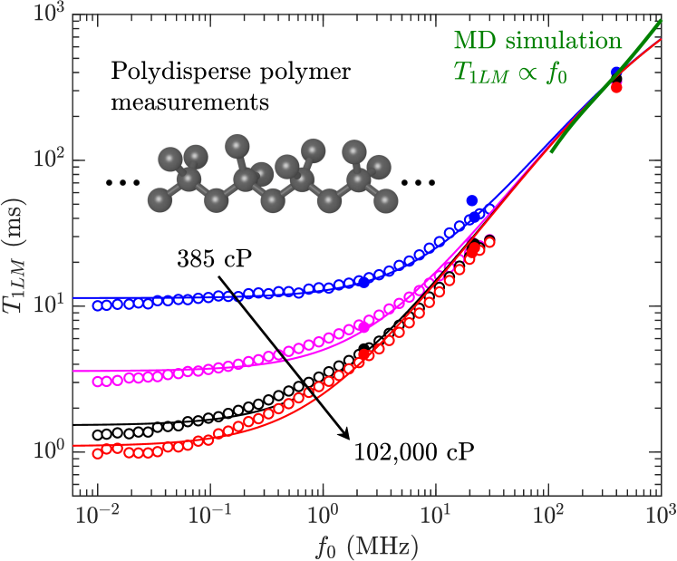
We previously showed that at high viscosities, the log-mean relaxation time for the polydisperse polymers becomes independent of viscosity and proportional to frequency singer:SPWLA2017 ; singer:EF2018 . This behavior presents significant deviations from the traditional Bloembergen, Purcell and Pound (BPP) model for 1H-1H dipole-dipole relaxation of monodisperse hard-spheres bloembergen:pr1948 where is predicted at high viscosities. Furthermore for the polydisperse polymers, we find that the “plateau” value normalized to = 2.3 MHz, 3 ms, is the same as previously reported bitumen data. This implies that the relaxation mechanism is independent of the paramagnetic concentration, and therefore that 1H-1H dipole-dipole relaxation dominates over paramagnetism at high viscosities.
This then lead us to develop a phenomenological model based on 1H-1H dipole-dipole relaxation which accounts for plateau at high viscosities by lowering the frequency exponent in the BPP model singer:SPWLA2017 ; singer:EF2018 . Lowering the frequency exponent implies a distribution in molecular correlation times of the viscous fluid, which is a similar approach to the phenomenological Cole-Davidson function davidson:jcp1951 ; lindesy:jcp1980 commonly used for dielectric and NMR data of glycerol flamig:jpcb2020 and monodisperse polymers kruk:pnmrs2012 . Our model also includes the presence of internal motions of the polymer branches through the Lipari-Szabo model lipari:jacs1982 ; lipari:jacs1982b .
In this study, we further test our model on polydisperse polymers using field cycling relaxometry and relaxation in the rotating frame. In the absence of paramagnetic impurities, we report on the anomalous viscosity dependence for the polydisperse polymers at high viscosity, where a similar anomalous behavior was previously reported for bitumen yang:petro2012 ; kausik:petro2019 . This again presents a significant departure from BPP where is predicted at high viscosities. We report on MD simulations of and by 1H-1H dipole-dipole relaxation of the polymer with viscosities in the range 1,000 cP. The MD simulations show that at high frequencies ( MHz), specifically 3 ms, in good agreement with measurements and our model at high viscosity. The MD simulations also confirm the dominance of intra-molecular over inter-molecular 1H-1H relaxation at high viscosity, which was previously only assumed to be the case.
II Methodology
II.1 Experimental
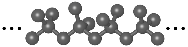
The polymers used in this study are listed in Table 1. The average molecular weight and poly-dispersivity index were measured using gel permeation chromatography (GPC) using an Agilent Technologies 1200 module. The data in Table 1 indicate that the polymers are highly dispersive, up to in the case of B360000 poly(isobutene). The large polydispersivity of the polymers make them ideal for comparing with crude-oils, which are also highly dispersed as evidenced by their wide distributions freedman:spe2001 . In the case of the three poly(isobutene) polymers in Table 1, the viscosity fit well to the functional form holden:japs1965 , with and in units of (cP) and (g/mol) at ambient singer:EF2018 . An illustration of a section of poly(isobutene) is shown in Fig. 2, which was used for molecular dynamics (MD) simulations.
| Name | Composition | (25∘C) | (40∘C) | ||
|---|---|---|---|---|---|
| (cP) | (cP) | (g/mol) | |||
| B1060 | Poly(1-decene) | 1,040 | 385 | 4,204 | 1.49 |
| B10200 | Poly(isobutene) | 10,700 | 4,060 | 2,256 | 2.13 |
| B73000 | Poly(isobutene) | 68,100 | 28,700 | 4,368 | 2.53 |
| B360000 | Poly(isobutene) | 333,000 | 102,000 | 9,436 | 3.11 |
The viscosity measurements were made using a Brookfield AMETEK viscometer. The viscosities did not depend on shear-rate (within experimental uncertainties), thereby making them suitable viscosity “standards” for comparing with NMR measurements which are measured at zero shear-rate. The viscosity measurements were made at both ambient temperature ( 25 ∘C) and at equilibrated temperatures of 40 ∘C using a circulation heat-bath. The viscosity data at 40 ∘C is used as a proxy for the NMR data at 38.4 ∘C.
A 1 GHz electron paramagnetic resonance (EPR) apparatus was used to measure the concentration of paramagnetic ions plus the (weight equivalent) concentration of free radicals (i.e. unpaired valence electrons), which both contribute to NMR paramagnetic relaxation. The EPR data on the Brookfield viscosity standards indicated ppm paramagnetic impurities (i.e. the signal was below the detection limit of the apparatus). The paramagnetic concentration in the polymers is at least an order of magnitude less than the estimated 1,000 ppm for Athabasca bitumen zhao:ef2007 ; singer:EF2018 .
1H NMR and measurements at a resonance frequency of = 2.3 MHz were made with a GeoSpec2 from Oxford Instruments, with a 29 mm diameter probe. The samples were measured at ambient conditions ( 25∘C) and after temperature equilibration to 30∘C. Additional measurements at 35∘C were made by turning off the chiller and equilibrating to the magnet temperature. and measurements at = 22 MHz and 30∘C were made with a special spectrometer from MR Cores at Core Laboratories, with a 30 mm diameter probe. and measurements at = 400 MHz at 25∘C were made with a Bruker Avance spectrometer, in a 5 mm diameter probe.
1H NMR , , and measurements at = 21 MHz and 38.4∘C were made at IFP-EN on a Maran Ultra, with a 18 mm diameter probe. The measurements in the rotating frame kimmich:book ; steiner:cpl2010 were made with a spin-locking frequency 1.7 kHz 42 kHz. Field cycling measurements were made on a Stelar fast field-cycling (FC) relaxometer from 30 MHz at 38.4∘C, with a 10 mm diameter probe. All of the above measurements were measured using a CPMG sequence with echo spacings of ms or less, except at = 400 MHz where was estimated from , where is the width of the NMR spectrum. The hydrogen index ( 1.17) of the polymers is discussed in singer:EF2018 .
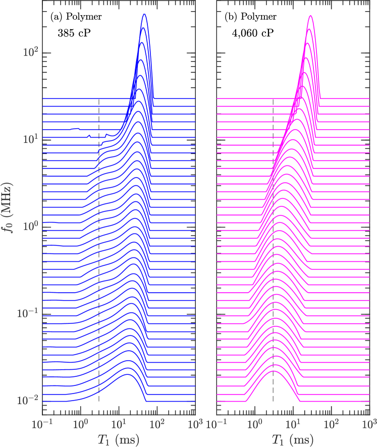
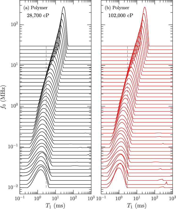
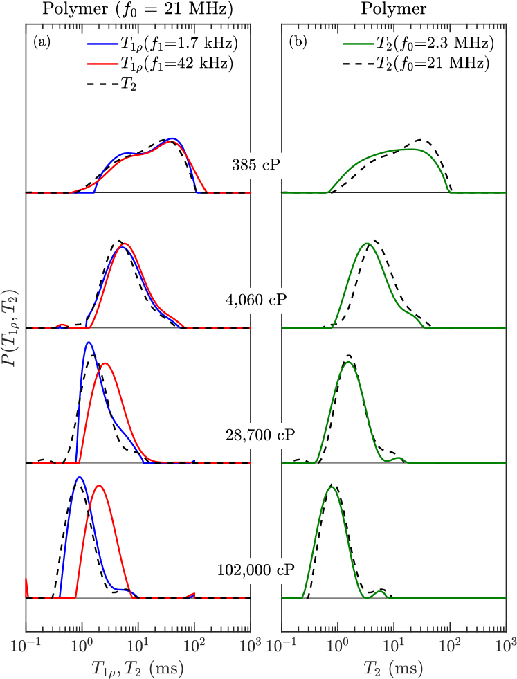
The , , and distributions of the pure polymers were determined using inverse Laplace transforms venkataramanan:ieee2002 ; song:jmr2002 . The FC distributions shown in Figs. 3 and 4 tend to narrow with increasing frequency due to larger (absolute) longitudinal cross-relaxation kalk:jmr1976 ; kowalewski:book (a.k.a. spin-diffusion). Figs. 3 and 4 also show the finite ramp-time of 3 ms required to ramp the field up and down. While in theory this does not effect the acquisition kimmich:pnmrs2004 , it has been noted that it does effect broad distributions with fast relaxing components roos:jbio2015 ; ward:jpc2018 . Our relaxation model indicates that this is likely the case for the 102,000 cP polymer, where the log-mean is most likely overestimated by a factor at low frequencies.
The distributions at = 1.7 kHz and = 42 kHz are shown in Fig. 5, alongside the distribution. and distributions tend to narrow with increasing viscosity, which is opposite to the trend in polydispersivity index in Table 1. The narrowing may therefore be a result of larger transverse cross-relaxation (in the low frequency limit) with increasing viscosity (i.e. increasing correlation time) kowalewski:book . In the case of the most viscous polymer, Fig. 5 shows that increases when going from = 1.7 kHz to 42 kHz, indicating the presence of molecular correlation times shorter than 1 s.
The log-mean values , and of the distributions are used for data analysis and fitting to the model, where for example , which is justified from the constituent viscosity model freedman:spe2001 . As shown in the Supporting Information, the effects of dissolved oxygen on as a function of frequency were measured for -heptane, and the concentration of dissolved oxygen in the polymer-heptane mix was predicted by MD simulations. The results indicate that the effects of dissolved oxygen on (and ) are negligible for all the polymers at all frequencies.
II.2 Relaxation model
The underlying expressions for , and in an isotropic system are given by mcconnell:book ; cowan:book :
| (1) | ||||
is the spectral density at the resonance frequency . The expression for in the rotating frame, , is similar to except that the zero-frequency term is replaced by where is the spin-locking frequency kimmich:book . Note that Eq. 1 does not assume a model for the spectral density .
II.2.1 BPP model
The BPP model for the spectral-density for intra-molecular 1H-1H dipole-dipole relaxation is given by the following bloembergen:pr1948 :
| (2) | ||||
| (3) | ||||
| (4) |
The BPP model assumes the Stokes-Einstein-Debye relation for hard spheres, where is the rotational correlation-time, is viscosity over temperature, and is the Stokes radius. The constant is the “second-moment” (i.e. the strength) of the intra-molecular 1H-1H dipole-dipole interactions (where is the 1H-1H distance between pairs and ). Note that the BPP model is only valid in the motional-narrowing regime where cowan:book , which is assumed to be the case throughout.
The BPP model introduces the important concept of the fast-motion (i.e. low viscosity) regime () where :
| (5) |
and the slow-motion (i.e. high viscosity) regime () where :
| (6) | ||||
| (7) |
II.2.2 New relaxation model
The BPP model fails for polydisperse polymers and bitumen at high-viscosity. In particular, BPP predicts that at high-viscosities, while measurements clearly indicate that is independent of viscosity. As such, a phenomenological model was developed where the frequency exponent in Eq. 2 is lowered from the BPP value to . This has the effect of dropping (and therefore ) out of the equation in the slow-motion regime () singer:SPWLA2017 ; singer:EF2018 . In the Supporting Information, we show that our model for the frequency exponent is similar to the limiting case of the phenomenological Cole-Davidson function commonly used for dielectric data for glycerol davidson:jcp1951 ; lindesy:jcp1980 , as well as for NMR data of glycerol and monodisperse polymers kruk:pnmrs2012 .
The consequence of changing the frequency exponent is to introduce a distribution in local rotational correlation times . This is justified by Woessner’s theories which show that as the molecule becomes less spherical, the internal motions in the molecule become more complex, and the distribution in correlation times becomes more pronounced woessner:jcp1962 ; woessner:jcp1965 . We also note that according to Woessner’s theories, simple fluids show a large distribution in correlation times when their motion is restricted by nano-confinement orazio:prb1990 .
Besides changing the frequency exponent, our model also allows for the existence of internal motions of non-rigid polymers using the Lipari-Szabo (LS) model lipari:jacs1982 ; lipari:jacs1982b . Changing the frequency exponent to in the BPP model and applying the LS model results in the following spectral density:
| (8) |
where the subscript in refers to the “Plateau”, and is assumed. is defined as the slow rotational correlation-time of the whole polymer molecule, which depends on viscosity. The order parameter is a measure of the rigidity of the polymer molecule, where = 1 for completely rigid molecules with no internal motion of the polymer branches, and = 0 for completely non-rigid molecules with full internal motion of the polymer branches. is the local correlation-time, which characterizes the fast ( 10’s ps) motions of the polymer branches.
Eq. 8 predicts the following expression in the slow-motion () regime:
| (9) |
which leads to the following approximation for :
| (10) |
In other words, the leading order term is , which is independent of viscosity. A deviation from linearity occurs at high frequencies when . This turns out to be more prominent for bitumen than for the polydisperse polymers, where is larger for bitumen (see below). We note that the temperature dependence of is most likely present but much less than the temperature dependence of (which depends on viscosity).
Eq. 8 also predicts the following approximation for in the slow-motion regime:
| (11) | ||||
The phenomenological relation is introduced in korb:jpcc2015 ; kausik:petro2019 , which relates to the Stokes-Einstein-Debye correlation time (Eq. 3) at high viscosities. is a constant, which leads to the prediction that , in agreement with previously published bitumen data yang:petro2012 ; kausik:petro2019 and the polydisperse polymer data shown below.
Two theories have been proposed for the relation at high viscosity. The first theory by Korb et al. korb:jpcc2015 stipulates that (referred to as in korb:jpcc2015 ) corresponds to a quasi-1D translational diffusion time of a maltene molecule within the transient nano-porous network of quasi immobile asphaltene macro-aggregates. below a critical viscosity (with 300 cP), while is constant above the critical viscosity . While korb:jpcc2015 uses this theory in the context of paramagnetism, their model for can also apply here in the context of 1H-1H dipole-dipole relaxation. The second theory kausik:petro2019 arrives at the same dependence of at high viscosity, but (referred to as in kausik:petro2019 ) is dominated by the maltene’s residence time in the asphaltene cluster (i.e. ), which is independent of viscosity.
Finally we note that the expression for (Eq. 11) contains the factor 10/3, implying that is in the fast-motion regime (i.e. independent of frequency) even when . This is motivated by the interpretation of the polydisperse polymer and bitumen data presented below.
II.3 MD simulations
Molecular dynamics (MD) simulations of monodisperse polymers were conducted. Four different chain lengths of poly(isobutene) (see Fig. 2) were simulated at 25∘C: a 16-mer, 8-mer, 4-mer and 2-mer. The viscosity of the 16-mer and 8-mer were estimated using the relation holden:japs1965 , with and in units of (cP) and (g/mol) at ambient singer:EF2018 . For example, in the case of the 16-mer where g/mol, this predicts a viscosity of 1,000 cP. The viscosities of the 4-mer and 2-mer were predicted using the empirical relation lo:SPE2002 in units of (ms) and (cP/K).
MD simulations of the intra-molecular () bloembergen:pr1948 and inter-molecular () torrey:pr1953 ; hwang:JCP1975 1H-1H dipole-dipole relaxation were then computed for the polymers, from which the total relaxation times () are calculated:
| (12) |
The procedure for the MD simulations are the same as reported elsewhere singer:jmr2017 ; asthagiri:seg2018 ; singer:jcp2018 , and details are given in the Supporting Information.
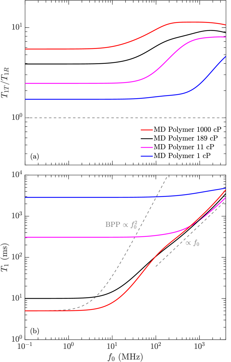
Fig. 6(a) shows the ratio of inter-molecular to intra-molecular relaxation times as a function of frequency for the four polymers. A value larger than unity indicates that intra-molecular relaxation dominates, while indicates that inter-molecular relaxation dominates. We find that increases with increasing viscosity, implying that intra-molecular relaxation dominates (by at least an order of magnitude) at high viscosities ( 1,000 cP). (not shown) show similar results. These findings justify the assumption in our model (Eq. 8) that intra-molecular relaxation dominates over inter-molecular relaxation.
Fig 6(b) shows the total relaxation (Eq. 12) as a function of frequency for the four polymers. The lowest viscosity (1 cP) polymer shows high values and minimal dispersion (i.e. minimal frequency dependence). On the other hand, the highest viscosity polymers show significant dispersion. The 189 cP and 1,000 cP polymers merge above 100 MHz into a linear relation . This behavior is exactly predicted by the model (Eq. 10), namely that is independent of viscosity. The 100 MHz region for the 1,000 cP polymer is compared with measurements and the model below.
We note that a similar relation was previously reported from MD simulations of heptane confined in a polymer matrix, where the surface relaxation of heptane followed under confinement parambathu:arxiv2020 . This implies a connection between the molecular dynamics of high-viscosity fluids and low-viscosity fluids under confinement.
III Results and Discussions
The results and interpretation are organized as follows. In section A we present the data for polydisperse polymers and bitumen in the slow-motion (i.e. high-viscosity) regime, and we use Eq. 10 to extract the free parameters and (Table 2). In section B we present the data for polydisperse polymers and bitumen in the slow-motion (i.e. high-viscosity) regime, and we use Eq. 11 to extract the free parameter (Table 2). In section C we present the full frequency dependence of and data for the polydisperse polymers spanning both the fast- and slow-motion regimes, and we use the full expression Eq. 8 to extract for each polymer (Table 3).
III.1 for polydisperse polymers and bitumen
The results for for crude oils (including bitumen) and polydisperse polymers are shown in Fig. 7(a). The crude-oil data are taken from various sources listed in the legend. The most recent addition is the bitumen data at 400 MHz by Kausik et al. kausik:petro2019 , measured over a range of temperatures (30∘C 90∘C).
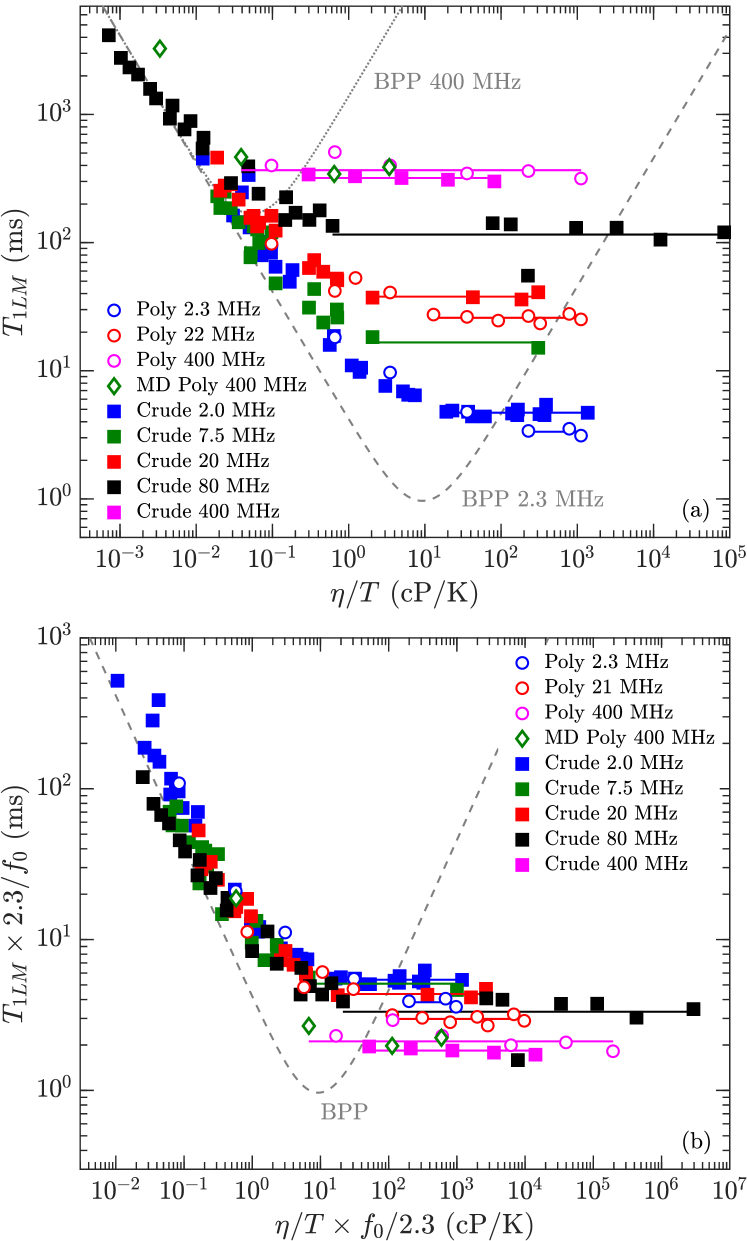
Also shown in Fig. 7(a) is the BPP prediction bloembergen:pr1948 at = 2.3 MHz and 400 MHz from Eq. 2. The crude oils roughly follow the BPP prediction at low viscosities, however clearly plateaus at high viscosity. Also shown are the MD simulations at 400 MHz for the polymers, which are consistent with the polydisperse polymer measurements.
Fig. 7(b) shows the same data as Fig. 7(a) but on a frequency normalized scale. More specifically, the -axis () is multiplied by with in units of MHz, while the -axis () is divided by . Frequency normalizing has the effect of collapsing the frequency dependence of the BPP model onto one universal curve zhang:spwla2002 . It also has the effect of collapsing the bitumen and polymer data in the slow-motion regime onto one plateau value given by 3 ms, i.e. . The more recent bitumen data at 400 MHz shows a slight departure from the low frequency data, namely the plateau value is lower than at lower frequencies. As shown below, the model takes this departure into account with the term in Eq. 10.
Fig. 8 shows data for the polydisperse polymers and the bitumen in the slow-motion regime (i.e. high-viscosity) regime, which corresponds to data within the horizontal lines (the log-average) in Fig. 7(a). The best fit to the new model using Eq. 9 and Eqs. 1 are shown for both polydisperse polymers and bitumen, and the best fit parameters are shown in Table 2. The second moment is fixed to = 20.0 kHz, which is the value for -heptane singer:EF2018 . A Stokes radius of 1.85 Å is used for the polymers, which is the value needed to match the correlation in the low-viscosity regime lo:SPE2002 . A slightly larger Stokes radius of 2.47 Å is used, which is the value needed to match the correlation in the low-viscosity regime freedman:spe2001 .
We note that the fact that are consistent with a constant Stokes radius in the low-viscosity regime, i.e. is independent of molecular size (and therefore viscosity), clearly shows that are probes of the local molecular dynamics. This is in stark contrast to the radius of gyration which depends on the molecular size singer:jmr2017 .
The first free-parameter in the model is the order parameter , which characterizes the rigidity of the molecule. is found for the polydisperse polymers, which is consistent with previously reported data for monodisperse polymers at high molecular-weights 4,000 g/mol graf:prl1998 ; kariyo:prl2006 ; kariyo:macro2008b . The fit to bitumen indicates a lower , implying a less-rigid molecule (i.e. more isotropic internal-motions). The second free-parameter is the local correlation-time , which characterizes the fast ( 10’s ps) motions of the molecular branches. The fit indicates a local correlation time of ns for the polydisperse polymers, and a longer ns for bitumen. We note that unlike bitumen, the fit for the polydisperse polymers is not very sensitive to , therefore an upper bound ns may be more appropriate for the polydisperse polymers.
| (kHz) | () | (ps) | (ns) | ||
|---|---|---|---|---|---|
| Bitumen | 20 | 2.47 | 0.085 | 53 | 268 |
| Polymer | 20 | 1.85 | 0.147 | 20 | 42 |
Also shown in Fig. 8 are the MD simulations of the 1,000 cP polymer above 100 MHz, corresponding viscosity independent region (see Fig. 6) where . The agreement between simulation and data/model in Fig. 8 is remarkable given that only a monodisperse model of poly(isobutene) is used in the simulations. This suggests that the behavior is generic at high-viscosities, and that 1H-1H dipole-dipole relaxation dominates over paramagnetism at high-viscosities.
III.2 for polydisperse polymers and bitumen
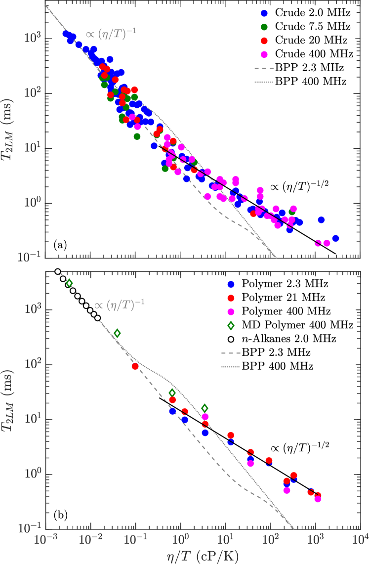
The results for for the crude oils are shown in Fig. 9(a), taken from various sources listed in the legend, with the most recent addition is the bitumen data at 400 MHz by Kausik et al. kausik:petro2019 . for the polydisperse polymers are shown in Fig. 7(b), along with de-oxygenated -alkane data shikhov:amr2016 , and the MD simulation results for the polymers at 400 MHz.
Solid lines are fits using the model in Eq. 11 with fitting parameters shown in Table 2, restricted to the high-viscosity region cP/K, or cP at ambient equivalently. Both the polydisperse polymers and bitumen data are consistent with for viscosities higher than cP/K. The model indicates that is a factor 6 larger for bitumen than for the polydisperse polymers. As discussed in Section II.2.2, there are two explanations for and the interpretation of constant korb:jpcc2015 ; kausik:petro2019 , and more investigations are required to narrow down the theory.
The BPP model predicts a “kink” in during the transition from the low- to high-viscosity regimes, where is shifted up by a factor 10/3 with increasing viscosity. The kink is supposed to occur at a viscosity corresponding to , which as shown in Fig. 9 predicts am intermittent spread between low frequency (2.3 MHz) and high frequency (400 MHz) data. However, no spread between the 2.3 MHz and 400 MHz data is apparent (within uncertainties), for both polydisperse polymers and bitumen. In other words, there is no apparent frequency dependence in (within uncertainties) during the low- to high-viscosity regime, at least up to 400 MHz. We also note that such a kink in has never been reported before for polydisperse fluids with a broad distribution.
We also note that the MD simulations of the polymers agree well with the measurements, which again suggests that 1H-1H dipole-dipole relaxation dominates over paramagnetism at high-viscosities.
III.3 Full frequency dependence of polydisperse polymer
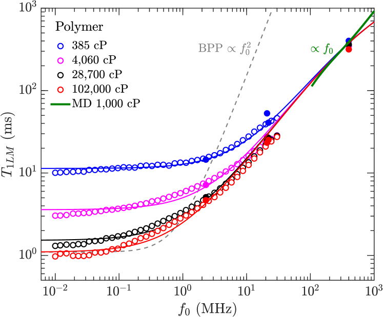
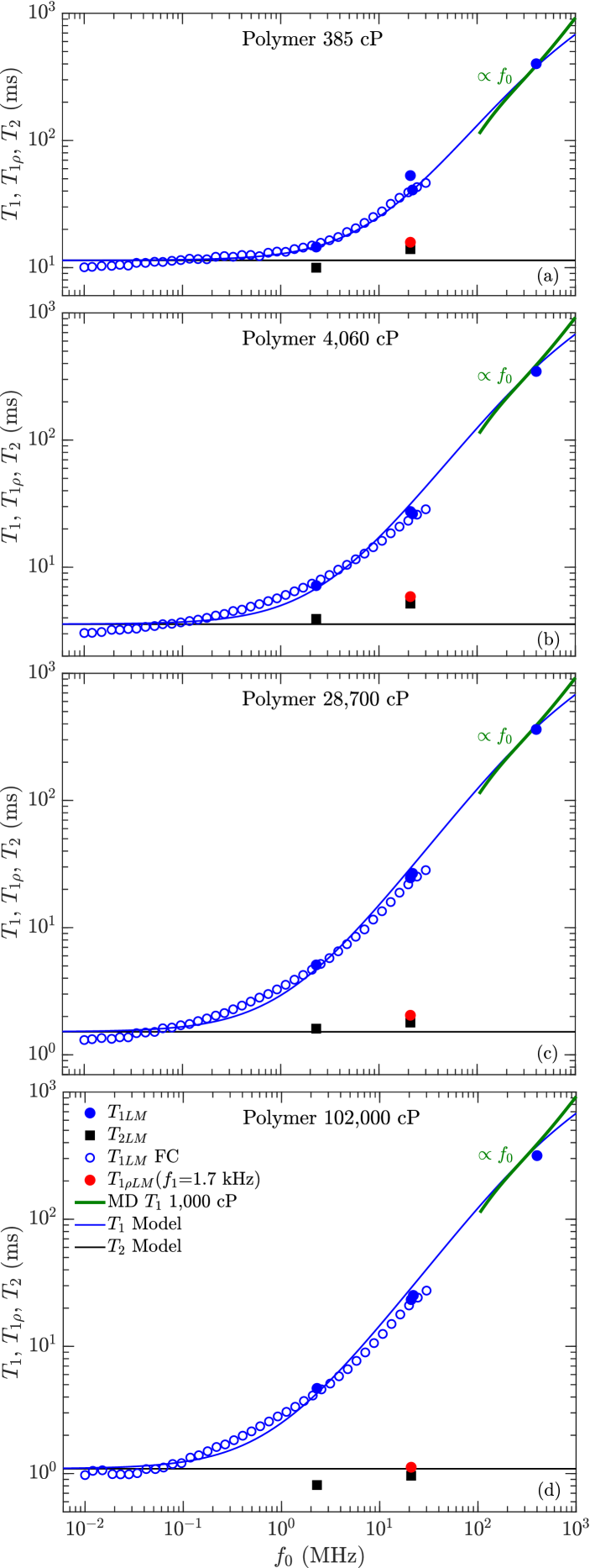
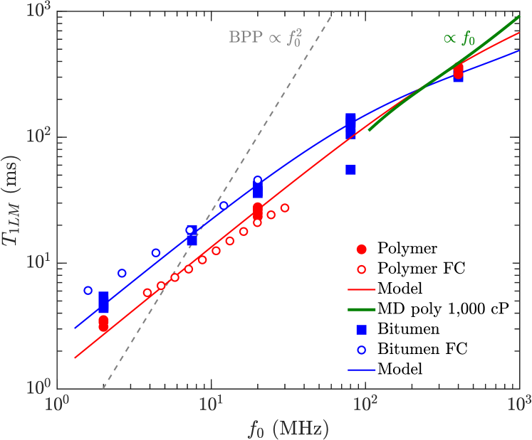
The full frequency dependence in for the polydisperse polymer are presented in Fig. 10. Also shown are the fits from the full expression of the model in Eq. 8 using fixed values of and listed in Table 2, and optimized values of listed in Table 3. The optimized values of in Table 3 tend to decrease with increasing viscosity, however the average agrees with the value in Table 2 determined from the entire set of data. The factor 2 smaller (and factor smaller ) for 102,000 cP is likely due to FC ramp-time effects which overestimate by a factor .
| All at | ||||
|---|---|---|---|---|
| 40∘C | (cP) | (ns) | (ns) | (ns) |
| 385 | 2 | 53 | 11 | |
| 4,060 | 25 | 51 | 36 | |
| 28,700 | 179 | 40 | 85 | |
| 102,000 | 636 | 22∗ | 118∗ |
The full expression of the model shows good agreement with the data over the entire frequency range MHz, including the coalescence at high frequencies corresponding to the slow-motion regime . Likewise, the MD simulation of the 1,000 cP polymer above 100 MHz shows behavior, consistent with the data and the model.
Fig. 11 shows the same data as Fig. 10, along with and (at = 1.7 kHz) which show similar values to at = 0.01 MHz. This implies that and ( = 1.7 kHz) have no dependence on (within uncertainties), and remain in the fast-motion regime even when . We speculate this is due to the broad distribution in correlation times, which for is more efficiently narrowed by longitudinal cross-relaxation (a.k.a. spin-diffusion) than for by transverse cross-relaxation. This stems from the fact that transverse cross-relaxation for is only effective in the “non-secular” limit, i.e. the low frequency limit kowalewski:book . As such, we speculate that the transition from the fast- to slow-motion regime may occur over a much broader frequency range for than for . This is supported by the lack of frequency dependence (i.e. the lack of a kink) in shown in Fig. 9(b). As such, we retain the factor 10/3 in Eq. 11 even in the slow-motion regime, at least up to 400 MHz.
IV Conclusions
We present NMR relaxation measurements of polydisperse polymers over a wide range of viscosities and over a wide range of frequencies using and in static fields, field-cycling relaxometry, and relaxation in the rotating frame.
We develop a phenomenological model to fit the relaxation data which accounts for a distribution in molecular correlation times for these polydisperse polymers by decreasing the frequency exponent in the BPP model bloembergen:pr1948 from to singer:SPWLA2017 ; singer:EF2018 . Our model also accounts for internal motions of the non-rigid polymer branches with a Lipari-Szabo model incorporating an order parameter (i.e. rigidity), and a (fast) local correlation time of the polymer branches. In the high viscosity regime of the model, the (slow) rotational correlation time of the entire polymer is taken to be , where is the Stokes-Einstein-Debye correlation time, and is a constant interpreted in korb:jpcc2015 ; kausik:petro2019 .
In the high-viscosity (i.e. slow-motion) regime, the model accounts for the viscosity independent “plateau” 3 ms of the polydisperse polymers. The model accounts for previously reported bitumen data where the same plateau was reported, as well as the departure from the behavior at high frequencies 100 MHz. The model also accounts for the behavior at high viscosities 0.3 cP/K (or 100 cP at ambient, equivalently), for both polydisperse polymers and bitumen.
The model is applied to the full range of frequencies covering both the fast- and slow-motion regimes of the polydisperse polymers. The data indicate that the and are independent of up to 400 MHz, which we speculate is because the transition from the fast- to slow-motion regime occurs over a much broader frequency range for than for . We speculate this may be a result of the broad distribution in correlation times together with cross-relaxation (a.k.a. spin-diffusion) effects.
Molecular dynamics simulations of and by 1H-1H dipole-dipole relaxation of monodisperse polymers are reported with viscosities in the range 1,000 cP. The simulations confirm the dominance of intra-molecular over inter-molecular 1H-1H relaxation at high viscosity, which was previously only assumed to be the case. The simulations for 100 cP show that at high frequencies ( MHz), specifically 3 ms, in good agreement with measurements and the model. A similar dispersion relation was previously reported from MD simulations of the surface relaxation of heptane confined in a polymer matrix, specifically 7 ms parambathu:arxiv2020 , implying a common NMR relaxation mechanism between high-viscosity fluids and low-viscosity fluids under confinement. The MD simulations also imply that 1H-1H dipole-dipole relaxation dominates over paramagnetism for these systems.
Supporting information
-
1.
Effects of dissolved oxygen.
-
2.
Details of the new model.
-
3.
Link between model and Cole-Davidson.
-
4.
Details of the MD simulation.
Acknowledgments
We thank the Chevron Corporation, the Rice University Consortium on Processes in Porous Media, and the American Chemical Society Petroleum Research Fund (No. ACS PRF 58859-ND6) for funding this work. We gratefully acknowledge the National Energy Research Scientific Computing Center, which is supported by the Office of Science of the U.S. Department of Energy (No. DE-AC02-05CH11231) and the Texas Advanced Computing Center (TACC) at The University of Texas at Austin for HPC time and support. We also thank Zeliang Chen, Maura Puerto, Lawrence B. Alemany, Kairan Zhu, Z. Harry Xie, Tuan D. Vo, Prof. Aydin Babakhani, Prof. Rafael Verduzco, Hao Mei, and Jinlu Liu for their contributions to Ref. singer:EF2018 , which paved the way for the further investigations reported here.
References
- (1) Zega, J. A.; House, W. V.; Kobayashi, R. A corresponding-states correlation of spin relaxation in normal alkanes Physica A 1989 156 (1), 277–293
- (2) Vinegar, H. J.; Tutunjian, P. N.; Edelstein, W. A.; Roemer, P. B. Whole-core analysis by 13C NMR Soc. Petrol. Eng. J. 1991 6 (2), 183–189
- (3) Tutunjian, P. N.; Vinegar, H. J. Petrophysical applications of automated high-resolution proton NMR spectroscopy Log Analyst 1992 136–144
- (4) Morriss, C. E.; Freedman, R.; Straley, C.; Johnson, M.; Vinegar, H. J.; Tutunjian, P. N. Hydrocarbon saturation and viscosity estimation from NMR logging in the belridge diatomite Log Analyst 1997 38 (2), 44–72
- (5) Zhang, Q.; Lo, S.-W.; Huang, C. C.; Hirasaki, G. J.; Kobayashi, R.; House, W. V. Some exceptions to default NMR rock and fluid properties Soc. Petrophys. Well Log Analysts 1998 SPWLA–1998–FF
- (6) LaTorraca, G. A.; Stonard, S. W.; Webber, P. R.; Carlson, R. M.; Dunn, K. J. Heavy oil viscosity determination using NMR logs Soc. Petrophys. Well Log Analysts 1999 SPWLA–1999–PPP
- (7) Appel, M.; Freeman, J. J.; Perkins, R. B.; van Dijk, N. P. Reservoir fluid study by nuclear magnetic resonance Soc. Petrophys. Well Log Analysts 2000 SPWLA–2000–HH
- (8) Freedman, R.; Lo, S.; Flaum, M.; Hirasaki, G. J.; Matteson, A.; Sezginer, A. A new NMR method of fluid characterization in reservoir rocks: Experimental confirmation and simulation results Soc. Petrol. Eng. J. 2001 6 (4), 452–464
- (9) Lo, S.-W.; Hirasaki, G. J.; House, W. V.; Kobayashi, R. Mixing rules and correlations of NMR relaxation time with viscosity, diffusivity, and gas/oil ratio of methane/hydrocarbon mixtures Soc. Petrol. Eng. J. 2002 7 (1), 24–34
- (10) Zhang, Y.; Hirasaki, G. J.; House, W. V.; Kobayashi, R. Oil and gas NMR properties: the light and heavy ends Soc. Petrophys. Well Log Analysts 2002 SPWLA-2002-HHH
- (11) Bryan, J.; Mirotchnik, K.; Kantzas, A. Viscosity determination of heavy oil and bitumen using NMR relaxometry J. Can. Petrol. Technol. 2003 42 (7), 29–34
- (12) Freedman, R.; Heaton, N.; Flaum, M.; Hirasaki, G. J.; Flaum, C.; Hürlimann, M. Wettability, saturation, and viscosity from NMR measurements Soc. Petrol. Eng. J. 2003 8 (4), 317–327
- (13) Hirasaki, G. J.; Lo, S.-W.; Zhang, Y. NMR properties of petroleum reservoir fluids Magn. Reson. Imaging 2003 21 (3-4), 269–277
- (14) Chen, S.; Zhang, G.; Kwak, H.; Edwards, C. M.; Ren, J.; Chen, J. Laboratory investigation of NMR crude oils and mud filtrates properties in ambient and reservoir conditions Soc. Petrol. Eng. 2004 SPE-90553-MS
- (15) Freedman, R.; Heaton, N. Fluid characterization using nuclear magnetic resonance logging Petrophysics 2004 45 (3), 241–250
- (16) Bryan, J.; Kantzas, A.; Bellehumeur, C. Oil-viscosity predictions from low-field NMR measurements Soc. Petrol. Eng. J. 2005 8 (1), 44–52
- (17) Winkler, M.; Freeman, J. J.; Appel, M. The limits of fluid property correlations used in NMR well logging: an experimental study of reservoir fluids at reservoir conditions Petrophysics 2005 46 (2), 104–112
- (18) Mutina, A. R.; Hürlimann, M. D. Effect of oxygen on the NMR relaxation properties of crude oils Appl. Magn. Reson. 2005 29:503
- (19) Nicot, B.; Fleury, M.; Leblond, J. A new methodology for better viscosity prediction using NMR relaxation Soc. Petrophys. Well Log Analysts 2006 SPWLA–2006–Z
- (20) Straley, C. Reassessment of correlations between viscosity and NMR measurements Soc. Petrophys. Well Log Analysts 2006 SPWLA–2006–AA
- (21) Freed, D. E. Dependence on chain length of NMR relaxation times in mixtures of alkanes J. Chem. Phys. 2007 126, 174502
- (22) Nicot, B.; Fleury, M.; Leblond, J. Improvement of viscosity prediction using NMR relaxation Soc. Petrophys. Well Log Analysts 2007 SPWLA–2007–U
- (23) Burcaw, L.; Kleinberg, R.; Bryan, J.; Kantzas, A.; Cheng, Y.; Kharrat, A.; Badry, R. Improved methods for estimating the viscosity of heavy oils from magnetic resonance data Soc. Petrophys. Well Log Analysts 2008 SPWLA–2008–W
- (24) Mutina, A. R.; Hürlimann, M. D. Correlation of transverse and rotational diffusion coefficient: a probe of chemical composition in hydrocarbon oils J. Phys. Chem. A 2008 112, 3291–3301
- (25) Yang, Z.; Hirasaki, G. J. NMR measurement of bitumen at different temperatures J. Magn. Reson. 2008 192, 280–293
- (26) Hürlimann, M. D.; Freed, D. E.; Zielinski, L. J.; Song, Y.-Q.; Leu, G.; Straley, C.; Minh, C. C.; Boyd, A. Hydrocarbon composition from NMR diffusion and relaxation data Petrophysics 2009 50 (2), 116–129
- (27) Lisitza, N. V.; Freed, D. E.; Sen, P. N.; Song, Y.-Q. Study of asphaltene nanoaggregation by nuclear magnetic resonance (NMR) Energy Fuels 2009 23, 1189–1193
- (28) Kantzas, A. Advances in magnetic resonance relaxometry for heavy oil and bitumen characterization J. Can. Petrol. Technol. 2009 48 (3), 15–23
- (29) Zielinski, L.; Saha, I.; Freed, D. E.; Hürlimann, M. D.; Liu, Y. Probing asphaltene aggregation in native crude oils with low-field NMR Langmuir 2010 26(7), 5014–5021
- (30) Zielinski, L.; Hürlimann, M. D. Nuclear magnetic resonance dispersion of distributions as a probe of aggregation in crude oils Energy Fuels 2011 25, 5090–5099
- (31) Yang, Z.; Hirasaki, G. J.; Appel, M.; Reed, D. A. Viscosity evaluation for NMR well logging of live heavy oils Petrophysics 2012 53 (1), 22–37
- (32) Jones, M.; Taylor, S. E.; Keng, H. Two-dimensional magnetic resonance study of synthetic oil sands Soc. Petrol. Eng. 2014 SPE-170006-MS
- (33) Chen, J. J.; Hürlimann, M. D.; Paulsen, J.; Freed, D.; Mandal, S.; Song, Y.-Q. Dispersion of and nuclear magnetic resonance relaxation in crude oils ChemPhysChem 2014 15, 2676–2681
- (34) Freedman, R.; Anand, V.; Grant, B.; Ganesan, K.; Tabrizi, P.; Torres, R.; Catina, D.; Ryan, D.; Borman, C.; Krueckl, C. A compact high-performance low-field NMR apparatus for measurements on fluids at very high pressures and temperatures Rev. Sci. Instrum. 2014 85, 025102
- (35) Benamsili, L.; Korb, J.-P.; Hamon, G.; Louis-Joseph, A.; Bouyssiere, B.; Zhou, H.; Bryant, R. G. Multi-dimensional nuclear magnetic resonance characterizations of dynamics and saturations of brine/crude oil/mud filtrate mixtures confined in rocks: The role of asphaltene Energy Fuels 2014 28, 1629–1640
- (36) Stapf, S.; Ordikhani-Seyedlar, A.; Ryan, N.; Mattea, C.; R.Kausik; Freed, D. E.; Song, Y.-Q.; Hürlimann, M. D. Probing maltene-asphaltene interaction in crude oil by means of NMR relaxation Energy Fuels 2014 28, 2395–2401
- (37) Korb, J.-P.; Vorapalawut, N.; Nicot, B.; Bryant, R. G. Relation and correlation between NMR relaxation times, diffusion coefficients, and viscosity of heavy crude oils J. Phys. Chem. C 2015 119 (43), 24439–24446
- (38) Vorapalawut, N.; Nicot, B.; Louis-Joseph, A.; Korb, J.-P. Probing dynamics and interaction of maltenes with asphaltene aggregates in crude oils by multiscale NMR Energy Fuels 2015 29, 4911–4920
- (39) Jones, M.; Taylor, S. E. NMR relaxometry and diffusometry in characterizing structural, interfacial and colloidal properties of heavy oils and oil sands Adv. Colloid Interface Sci. 2015 224, 33–45
- (40) Ordikhani-Seyedlar, A.; Neudert, O.; Stapf, S.; Mattea, C.; Kausik, R.; Freed, D. E.; Song, Y.-Q.; Hürlimann, M. D. Evidence of aromaticity-specific maltene NMR relaxation enhancement promoted by semi-immobilized radicals Energy Fuels 2016 30, 3886–3893
- (41) Shikhov, I.; Arns, C. Temperature-dependent oxygen effect on NMR - relaxation-diffusion correlation of -alkanes Appl. Magn. Reson. 2016 47 (12), 1391–1408
- (42) Singer, P. M.; Chen, Z.; Alemany, L. B.; Hirasaki, G. J.; Zhu, K.; Xie, Z. H.; Vo, T. D. NMR relaxation of polymer-alkane mixes, a model system for crude oils Soc. Petrophys. Well Log Analysts 2017 SPWLA-2017-XX
- (43) Singer, P. M.; Chen, Z.; Alemany, L. B.; Hirasaki, G. J.; Zhu, K.; Xie, Z. H.; Vo, T. D. Interpretation of NMR relaxation in bitumen and organic shale using polymer-heptane mixes Energy Fuels 2018 32 (2), 1534–1549
- (44) Kausik, R.; Freed, D.; Fellah, K.; Feng, L.; Ling, Y.; Simpson, G. Frequency and temperature dependence of 2D NMR - maps of shale Petrophysics 2019 60 (1), 37–49
- (45) Markovic, S.; Bryan, J. L.; Turakhanov, A.; Cheremisin, A.; Mehta, S. A.; Kantzas, A. In-situ heavy oil viscosity prediction at high temperatures using low-field NMR relaxometry and nonlinear least squares Fuel 2020 260, 116328
- (46) Washburn, K. E. Relaxation mechanisms and shales Concepts Magn. Reson. 2014 A 43 (3), 57–78
- (47) Singer, P. M.; Chen, Z.; Hirasaki, G. J. Fluid typing and pore size in organic shale using 2D NMR in saturated kerogen isolates Petrophysics 2016 57 (6), 604–619
- (48) Fleury, M.; Romero-Sarmiento, M. Characterization of shales using - maps J. Petrol. Sci. Eng. 2016 137, 55–62
- (49) Zhang, B.; Daigle, H. Nuclear magnetic resonance surface relaxation mechanisms of kerogen Geophysics 2017 82(6), 15–22
- (50) Washburn, K. E.; Cheng, Y. Detection of intermolecular homonuclear dipolar coupling in organic rich shale by transverse relaxation exchange J. Magn. Reson. 2017 278, 18–24
- (51) Tandon, S.; Heidari, Z. Improved analysis of NMR measurement in organic-rich mudrocks through qunatifying hydrogen-kerogen interfacial relaxation mechanisms Soc. Petrophys. Well Log Analysts 2019 SPWLA-2019-MMM
- (52) Xie, H.; Gan, Z. Investigation of physical properties of hydrocarbons in unconventional mudstines using two-dimensional NMR relaxometry Soc. Petrophys. Well Log Analysts 2019 SPWLA-2019-ZZZ
- (53) Parambathu, A. V.; Singer, P. M.; Hirasaki, G. J.; Chapman, W. G.; Asthagiri, D. Molecular dynamics simulations of NMR relaxation and diffusion of heptane confined in a polymer matrix 2020 arXiv:2001.07310 https://arxiv.org/abs/2001.07310
- (54) Liu, J.; Chapman, W. G. Thermodynamic modeling of the equilibrium partitioning of hydrocarbons in nanoporous kerogen particles Energy Fuels 2019 33 (2), 891–904
- (55) Abivin, P.; Taylor, S. D.; Freed, D. Thermal behavior and viscoelasticity of heavy oils Energy Fuels 2012 26, 3448–3461
- (56) Kariyo, S.; Gainaru, C.; Schick, H.; Brodin, A.; Novikov, V. N.; Rössler, E. A. From a simple liquid to a polymer melt: NMR relaxometry study of polybutadiene Physical Review Letters 2006 97, 207803
- (57) Kariyo, S.; Brodin, A.; Gainaru, C.; Herrmann, A.; Hintermeyer, J.; Schick, H.; Novikov, V. N.; Rössler, E. A. From simple liquid to polymer melt. glassy and polymer dynamics studied by fast field cycling NMR relaxometry: Rouse regime Macromolecules 2008 41, 5322–5332
- (58) Kruk, D.; Herrmann, A.; Rössler, E. Field-cycling NMR relaxometry of viscous liquids and polymers Prog. Nucl. Magn. Reson. Spect. 2012 63, 33–64
- (59) Graf, R.; Heuer, A.; Spiess, H. W. Chain-order effects in polymer melts probed by 1H double-quantum NMR spectroscopy Physical Review Letters 1998 80 (26), 5738–5741
- (60) Chávez, F. V.; Saalwächter, K. Time-domain NMR observation of entangled polymer dynamics: Universal behavior of flexible homopolymers and applicability of the tube model Macromolecules 2011 44, 1549–1559
- (61) Chávez, F. V.; Saalwächter, K. Time-domain NMR observation of entangled polymer dynamics: Analytical theory of signal functions Macromolecules 2011 44, 1560–1569
- (62) Mordvinkin, A.; Saalwächter, K. Microscopic observation of the segmental orientation autocorrelation function for entangled and constrained polymer chains J. Chem. Phys. 2017 146, 094902
- (63) Bloembergen, N.; Purcell, E. M.; Pound, R. V. Relaxation effects in nuclear magnetic resonance absorption Phys. Rev. 1948 73 (7), 679–712
- (64) Davidson, D. W.; Cole, R. H. Dielectric relaxation in glycerol, propylene glycol, and -propanol J. Chem. Phys. 1951 19, 1484
- (65) Lindsey, C. P.; Patterson, G. D. Detailed comparison of the Williams–Watts and Cole–Davidson functions J. Chem. Phys. 1980 73, 3348
- (66) Flämig, M.; Hofmann, M.; Fatkullin, N.; ; Rössler, E. A. NMR relaxometry: The canonical case glycerol J. Phys. Chem. B 2020 124, 1557–1570
- (67) Lipari, G.; Szabo, A. Model-free approach to the interpretation of nuclear magnetic resonance relaxation in macromolecules. 1. Theory and range of validity J. Amer. Chem. Soc. 1982 104, 4546–4559
- (68) Lipari, G.; Szabo, A. Model-free approach to the interpretation of nuclear magnetic resonance relaxation in macromolecules. 2. Analysis of experimental results J. Amer. Chem. Soc. 1982 104, 4559–4570
- (69) Holden, G. Viscosity of polyisoprene J. Appl. Polym. Sci. 1965 9, 2911–2925
- (70) Zhao, B.; Shaw, J. M. Composition and size distribution of coherent nanostructures in Athabasca bitumen and Maya crude oil Energy Fuels 2007 21, 2795–2804
- (71) Kimmich, R. NMR Tomography, Diffusometry and Relaxometry Springer-Verlag 1997
- (72) Steiner, E.; Yemloul, M.; Guendouz, L.; Leclerc, S.; Robert, A.; Canet, D. NMR relaxometry: Spin lattice relaxation times in the laboratory frame versus spin lattice relaxation times in the rotating frame Chem. Phys. Lett. 2010 495, 287–291
- (73) Venkataramanan, L.; Song, Y.-Q.; Hürlimann, M. D. Solving fredholm integrals of the first kind with tensor product structure in 2 and 2.5 dimensions IEEE Trans. Sig. Process. 2002 50 (5), 1017–1026
- (74) Song, Y.-Q.; Venkataramanan, L.; Hürlimann, M. D.; Flaum, M.; Frulla, P.; Straley, C. - correlation spectra obtained using fast two-dimensional laplace inversion J. Magn. Reson. 2002 154, 261–268
- (75) Kalk, A.; Berendsen, H. J. C. Proton magnetic relaxation and spin diffusion in proteins J. Magn. Reson. 1976 24, 343–366
- (76) Kowalewski, J.; Mäler, L. Nuclear Spin Relaxation in Liquids: Theory, Experiments, and Applications Taylor & Francis Group 2006
- (77) Kimmich, R.; Anoardo, E. Field-cycling NMR relaxometry Prog. Nucl. Magn. Reson. Spect. 2004 44, 257–320
- (78) Roos, M.; Hofmann, M.; Link, S.; Ott, M.; Balbach, J.; Rössler, E.; Saalwächter, K.; Krushelnitsky, A. The “long tail” of the protein tumbling correlation function: observation by 1H NMR relaxometry in a wide frequency and concentration range J. Biomol. NMR 2015 63, 403–415
- (79) Ward-Williams, J.; Korb, J.-P.; Gladden, L. F. Insights into functionality-specific adsorption dynamics and stable reaction intermediates using fast field cycling NMR J. Phys. Chem. C 2018 122, 20271–20278
- (80) McConnell, J. The Theory of Nuclear Magnetic Relaxation in Liquids Cambridge University Press 1987
- (81) Cowan, B. Nuclear Magnetic Resonance and Relaxation Cambridge University Press 1997
- (82) Woessner, D. E. Spin relaxation processes in a two-proton system undergoing anisotropic reorientation J. Chem. Phys. 1962 36 (1), 1–4
- (83) Woessner, D. E. Nuclear magnetic dipole-dipole relaxation in molecules with internal motion J. Chem. Phys. 1965 42 (6), 1855–1859
- (84) Orazio, F. D.; Bhattacharj, S.; Halperin, W. P.; Eguchi, K.; Mizusaki, T. Molecular diffusion and nuclear-magnetic-resonance relaxation of water in unsaturated porous silica glass Physical Review B 1990 42, 9810
- (85) Torrey, H. C. Nuclear spin relaxation by translational diffusion Phys. Rev. 1953 92 (4), 962–969
- (86) Hwang, L.-P.; Freed, J. H. Dynamic effects of pair correlation functions on spin relaxation by translational diffusion in liquids J. Chem. Phys. 1975 63 (9), 4017–4025
- (87) Singer, P. M.; Asthagiri, D.; Chapman, W. G.; Hirasaki, G. J. Molecular dynamics simulations of NMR relaxation and diffusion of bulk hydrocarbons and water J. Magn. Reson. 2017 277, 15–24
- (88) Asthagiri, D.; Singer, P. M.; Parambathu, A. V.; Chen, Z.; Hirasaki, G. J.; Chapman, W. G. Molecular dynamics simulations of NMR relaxation and diffusion of bulk hydrocarbons SEG/AAPG/EAGE/SPE Research and Development Petroleum Conference and Exhibition 2018 101–102
- (89) Singer, P. M.; Asthagiri, D.; Chen, Z.; Valiya Parambathu, A.; Hirasaki, G. J.; Chapman, W. G. Role of internal motions and molecular geometry on the NMR relaxation of hydrocarbons J. Chem. Phys. 2018 148 (16), 164507
- (90) Teng, C.-L.; Hong, H.; Kiihne, S.; Bryant, R. G. Molecular oxygen spin–lattice relaxation in solutions measured by proton magnetic relaxation dispersion J. Magn. Reson. 2001 148, 31–34
- (91) Lauffer, R. B. Paramagnetic metal complexes as water proton relaxation agents for NMR imaging: Theory and design Chem. Rev. 1987 87, 901–927
- (92) Abragam, A. Principles of Nuclear Magnetism Oxford University Press, International Series of Monographs on Physics 1961
- (93) Singer, P. M.; Asthagiri, D.; Chapman, W. G.; Hirasaki, G. J. NMR spin-rotation relaxation and diffusion of methane J. Chem. Phys. 2018 148 (20), 204504
- (94) Abramowitz, M.; Stegun, I. A. Handbook of Mathematical Functions with Formulas, Graphs, and Mathematical Tables chapter 5: Exponential integral and related functions Dover Publications (1983) edition 1964
- (95) Magin, R. L.; Li, W.; Velasco, M. P.; Trujillo, J.; Reiter, D. A.; Morgenstern, A.; Spencer, R. G. Anomalous NMR relaxation in cartilage matrix components and native cartilage: Fractional-order models J. Magn. Reson. 2010 210, 184–191
- (96) Beckmann, P. A. Spectral densities and nuclear spin relaxation in solids Phys. Rep. 1988 171 (3), 85–128
- (97) Phillips, J. C.; Braun, R.; Wang, W.; Gumbart, J.; Tajkhorshid, E.; Villa, E.; Chipot, C.; Skeel, R. D.; Kale, L.; Schulten, K. Scalable molecular dynamics with NAMD J. Comput. Chem. 2005 26(16), 1781–1802
- (98) Theoretical and Computational Biophysics group, NIH Center for Macromolecular Modeling and Bioinformatics, at the Beckman Institute, University of Illinois at Urbana-Champaign NAMD 2018 http://www.ks.uiuc.edu/Research/namd/
- (99) Vanommeslaeghe, K.; Hatcher, E.; Acharya, C.; Kundu, S.; Zhong, S.; Shim, J.; Darian, E.; Guvench, O.; Lopes, P.; Vorobyov, I.; Jr., A. D. M. CHARMM general force field: A force field for drug-like molecules compatible with the CHARMM all-atom additive biological force field J. Comput. Chem. 2010 31, 671–690
- (100) ParamChem CGenFF 3.0.1 https://cgenff.paramchem.org 2020
- (101) Bakhmutov, V. I. NMR Spectroscopy in Liquids and Solids CRC Press, Taylor & Francis Group 2015
V Supporting Information
V.1 Effects of dissolved oxygen
The measured of a bulk fluid at atmospheric conditions are given by the following:
| (13) |
are the bulk contributions from 1H-1H dipole-dipole relaxation. For de-oxygenated -alkanes at ambient it was previously shown that lo:SPE2002 , which for -heptane is = 7,320 ms at 25 ∘C (where = 0.39 cP).
Given the measured and the known for -heptane at ambient, Eq. 13 yields the paramagnetic contribution from dissolved oxygen. As shown in Fig. 12(a), increases from 2,500 ms at MHz to 5,600 ms at MHz. depends on the electron correlation time and the concentration of dissolved oxygen through the following relations mcconnell:book :
| (14) | ||||
| (15) |
where the BPP spectral density is given by:
| (16) |
is the electron correlation time of the paramagnetic O2 molecule, and the second moment (i.e. strength) is given by . Note that the Larmor frequency of the electron is larger than 1H by a factor . The BPP model for the spectral density was previously shown to work well for a variety of solvents of various molecular weights teng:jmr2001 . Fig. 12(a) shows that the fit to using Eqs. 14 and 16 work well, with best fit parameters ps (which is consistent with teng:jmr2001 ) and = 62.8 kHz.
Given that the concentration of dissolved oxygen in -heptane is 132 mg/L (or 4.12 mM equivalently) at ambient ( = 0.21 atm) implies that the relaxivity (defined in MRI terminology lauffer:cr1987 ) of O2 is mM-1s-1 at low frequencies 100 MHz.
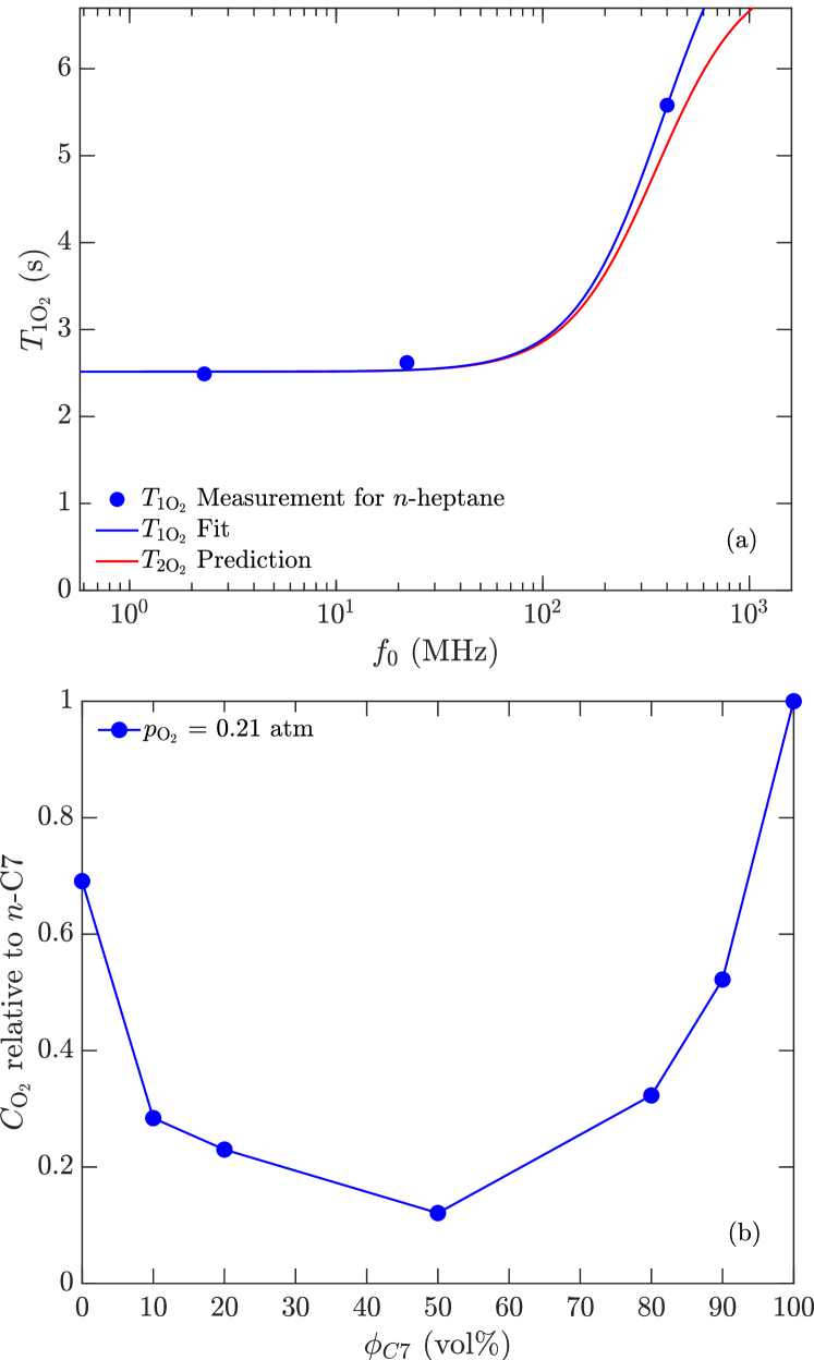
As shown in teng:jmr2001 , is roughly constant for solvents with the molecular weight of heptane or higher, and also appears roughly constant at lower molecular weights ward:jpc2018 . Furthermore as shown in Fig. 12(b), MD simulations indicate that is 30 % less for the 1,000 cP polymer than for heptane parambathu:arxiv2020 , implying that is 30 % larger for the polymer than for heptane. This predicts that 8,000 ms for the polymer at MHz, which is much larger than the measured 300 ms. In other words, the effects of oxygen on are negligible for the polymer at 400 MHz. Below 400 MHz, the effects of oxygen on the polymer are even less since the measured 300 ms.
The only cases in this report where the effects of dissolved oxygen are apparent are for the low-viscosity crude-oils at 100 MHz where 1,000 ms. In such cases deviate slightly from the BPP correlation line in the low-viscosity regime.
V.2 Details of the model
The autocorrelation function for fluctuating magnetic 1H-1H dipole-dipole interactions is central to the development of the NMR relaxation theory in liquids bloembergen:pr1948 ; torrey:pr1953 ; abragam:book ; hwang:JCP1975 ; mcconnell:book ; cowan:book ; kimmich:book . From , one can determine the spectral density function by Fourier transform as such:
| (17) |
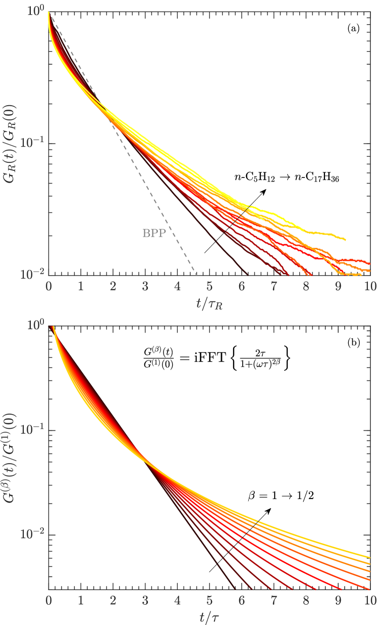
for in units of s-2 mcconnell:book . As shown in Fig. 13(a), for the -alkanes has a multi-exponential (i.e. “stretched”) decay rather than the single exponential decay predicted by BPP. Furthermore, the degree of stretching increases with increasing carbon number (i.e. increasingly non-spherical geometry). MD simulations indeed confirm that -pentane and -hexane have a more stretched intra-molecular autocorrelation function (i.e. a broader distribution of correlation times) than the symmetric neo-pentane and benzene molecules, respectively singer:jcp2018 . The degree of stretching can be further analyzed using inverse Laplace transforms (see also singer:jcp2018b and supporting information in singer:jcp2018 ).
By comparison, Fig 13(b) shows the effect of decreasing the exponent in the spectral density function as such:
| (18) | ||||
| (19) |
where the real part of the inverse Fourier transform is also defined. An analytical expression for exists for the two extreme cases:
| (20) | ||||
| (21) |
The case of , , is the BPP model with a single-exponential decay. The case of , abramowitz:1964 , is the stretched case used in the phenomenological model to account for the independence of on , i.e. the independence on . As demonstrated in Fig 13, increasing the carbon number increases the degree of stretching in Fig 13(a), which corresponds to decreasing in Fig 13(b).
It is interesting to note that the long time behavior of Eq. 21 is for . This is analogous to the Mittag-Leffler function, which starts off as a stretched exponential at short times, and turns into a power-law decay at long times magin:jmr2011 .
We note that starts to diverge below , therefore the model is valid for times . Correspondingly, this implies that the model for is valid for frequencies (where the factor 2 reflects the terms in Eq. 1). Given the local correlation-time ps, this corresponds to validity below frequencies 10 GHz.
V.3 Link between model and Cole-Davidson
The Cole-Davidson function is widely used to describe the dielectric response davidson:jcp1951 ; lindesy:jcp1980 ; beckmann:prep1988 and its departure from the traditional Debye model. The function is defined as such:
| (22) |
which reduces to the following expression:
| (23) |
The Cole-Davidson exponent is bound by , where is the Debye model. As is decreased, the underlying distribution in molecular correlation times grows wider.
The Cole-Davidson function has also been successfully used to describe NMR relaxation of glycerol and monodispersed polymers through the relation kruk:pnmrs2012 ; flamig:jpcb2020 . The NMR Cole-Davidson spectral density is given by the following:
| (24) |
which reduces to the following expression:
| (25) |
For the purposes of comparison with our model, we have added a factor to the definition of . The factor is related to the units convention of the spectral density cowan:book . The factor is introduced to highlight the similarity with our model. as defined in Eq. 25 becomes independent of in the limit , and tends towards:
| (26) |
In other words, tends towards our model (without the added Lipari-Szabo model, i.e. ) in the case of and . Fig 14 shows determined from for = 1, 0.6, and , compared with our model. The similarity between for and our model is remarkable, and only shows a 22% deviation at the transition from the fast- to slow-motion regime. The deviation for (not shown) 14% is even less.
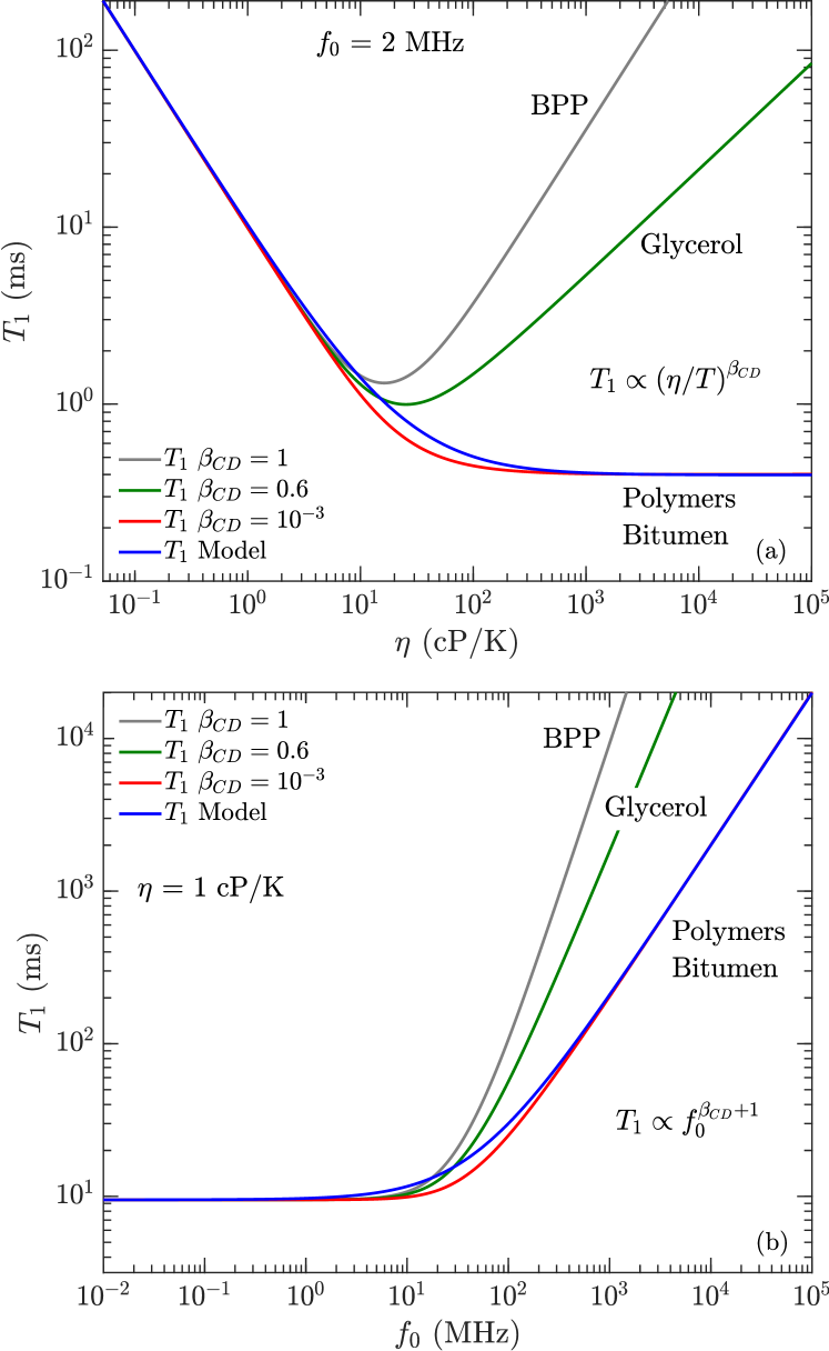
Fig 14 also indicates the corresponding cases as BPP ( = 1), glycerol ( 0.6 for the -peak davidson:jcp1951 ; kruk:pnmrs2012 ; flamig:jpcb2020 ), and our model for polydisperse polymers and bitumen (). Also shown are the limiting behavior in according to Cole-Davidson in the slow-motion regime .
The above comparison shows that polydisperse polymers and bitumen have a much larger distribution in molecular correlation times than gycerol. In terms of the Cole-Davidson model, this manifests itself as a small exponent for the polydisperse polymers and bitumen, compared to monodisperse gycerol where for the -peak.
V.4 Details of MD simulation
The detailed simulation procedure is provided in Ref. parambathu:arxiv2020 . The system was simulated using NAMD phillips:JCC2005 ; NAMD code, and modeled using CGenFF Force Fieldcgenff:2010 ; cgenff:2020 . The number of molecules used were 269, 143, 74, and 40 for the 2-mer, 4-mer, 8-mer and 16-mer, respectively. The systems were equilibrated at constant conditions at 25∘C and 1 atm. The data was then collected in a ensemble to compute the autocorrelations .
The results of the intra-molecular and inter-molecular are shown in Fig. 15(a) for the polymer at 1 cP and 1,000 cP. In order to quantify the departure of from single-exponential decay, we fit to a sum of multi-exponential decays and determine the underlying probability distribution in correlation times . More specifically, we perform an inversion of the following Laplace transform venkataramanan:ieee2002 ; song:jmr2002 ; singer:jcp2018 :
| (27) | ||||
| (28) | ||||
| (29) |
where are the probability distribution functions derived from the inversion, plotted in Fig. 15(b). Details of the inversion procedure can be found in singer:jcp2018b and in the supporting information in singer:jcp2018 .
The in Fig. 15(b) indicate a set of 5 polymer modes, located at similar values for both intra-molecular and inter-molecular interactions. The intra-molecular has an additional mode at short ps for both the polymer and heptane, while it is absent for in both cases. Similar observation of the ps mode was reported in the supporting information for all the liquid-state -alkanes singer:jcp2018 , and it is attributed to the fast rotation of the methyl groups.
The decomposition of into a sum of exponential decays is common practice in phenomenological models of complex molecules beckmann:prep1988 ; bakhmutov:book , where the more complex the molecular dynamics, the more exponential terms are required woessner:jcp1962 ; woessner:jcp1965 . This is in contrast to analytical techniques and theories used to interpret the autocorrelation function of monodisperse polymers with high molecular-weight 4,000 g/mol where entanglement occurs, and a power law decay is observed chavez:macro2011 ; chavez:macro2011b ; mordvinkin:jcp2017 . We note however that our polydisperse polymers most likely do not entangle to the extent that monodisperse polymers do, if indeed the polydisperse polymers entangle at all.
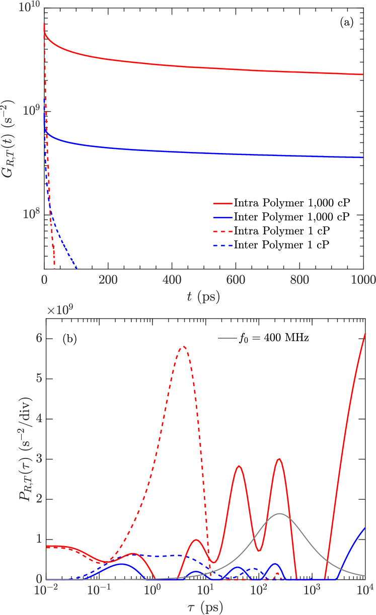
Also defined in Eq. 28 are the correlation times derived from , which are found to be = 2,380 ps and = 3,030 ps at 1,000 cP, compared with = 3.33 ps and = 10.1 ps at 1 cP. In other words, the MD simulations indicate that increase by a factor of 500 from 1 cP to 1,000 cP.
The spectral density is determined from the Fourier transform (Eq. 17) of (Eq. 27):
| (30) |
from which the dispersion (i.e. frequency dependence) can be determined as such:
| (31) | ||||
| (32) | ||||
| (33) |
Fig. 15(a) indicates that the second moment is about a factor 10 larger for intra-molecular () versus inter-molecular () interactions at 1,000 cP. Given that at 1,000 cP, one can then deduce that the ratio . In other words, the intra-molecular relaxation rate is larger than the inter-molecular relaxation rate, therefore intra-molecular relaxation dominates at 1,000 cP.
The gray curve in Fig. 15(b) corresponds to the “BPP frequency filter” defined in Eq. 30, at 400 MHz (as an example). In other words, the components of contributing to at 400 MHz are weighted by the BPP frequency filter curve, which peaks at . As such, the components in at long ps do not contribute to at 400 MHz (as an example), nor do the short components ps.