Emergence of hierarchical modes from deep learning
Chan Li1Haiping Huang1,2huanghp7@mail.sysu.edu.cn1PMI Lab, School of Physics,
Sun Yat-sen University, Guangzhou 510275, People’s Republic of China
2Guangdong Provincial Key Laboratory of Magnetoelectric Physics and Devices,
Sun Yat-sen University, Guangzhou 510275, People’s Republic of China
Abstract
Large-scale deep neural networks consume expensive training costs, but the training results in less-interpretable weight matrices constructing the networks.
Here, we propose a mode decomposition learning that can interpret the weight matrices as a hierarchy of latent modes. These modes are akin to patterns
in physics studies of memory networks, but the least number of modes increases only logarithmically with the network width, and becomes even a constant when the width further grows.
The mode decomposition learning not only saves a significant large amount of training costs, but also explains the network performance with
the leading modes, displaying a striking piecewise power-law behavior.
The modes specify a progressively compact latent space across the network hierarchy, making a more disentangled subspaces compared to standard training.
Our mode decomposition learning is also studied in an analytic on-line learning setting, which reveals multi-stage of learning dynamics with a continuous specialization of hidden nodes.
Therefore, the proposed mode decomposition learning
points to a cheap and interpretable route towards the magical deep learning.
Introduction.—
Deep neural networks are dominant tools with a broad range of applications in not only image and language processing,
but also scientific researches Goodfellow et al. (2016); Carleo et al. (2019). These networks are parameterized by a huge amount of trainable weight matrices, thereby consuming
an expensive training cost. However, these weight matrices are hard to interpret, and thus mechanisms underlying the macroscopic performance of the networks remain
a big mystery in theoretical studies of neural networks Huang (2022); Roberts et al. (2022).
To save the computational cost, previous studies of deep networks applied singular value decomposition to the weight matrices Jaderberg et al. (2014); Yang et al. (2020); Giambagli et al. (2021); Chicchi et al. (2021).
This decomposition requires the orthogonality condition for the singular vectors and positive singular values. The training also involves a carefully-designed
structure for the trainable decomposition scheme Giambagli et al. (2021); Chicchi et al. (2021). These constraints and designs make the training process complicated, and thus a concise physics interpretation is still lacking.
In addition,
previous studies of recurrent memory networks showed that
the network weight can be decomposed into separate random orthogonal patterns with corresponding importance scores Jiang et al. (2021); Zhou et al. (2021). Inspired by these studies,
we conjecture that the learning in deep networks is shaped by a hierarchy of latent modes, which are not necessarily orthogonal,
and the weight matrix can be expressed by these modes.
The mode decomposition learning (MDL)
leads to a progressively compact latent mode space across the network hierarchy,
and meanwhile the subspaces corresponding to different types of input are strongly disentangled, facilitating discrimination.
The least number of latent modes achieving the comparable performance with the costly standard methods grows
only logarithmically with the network width and even could be a constant, thereby reducing significantly the training cost.
The mode spectrum exhibits an intriguing
piecewise power-law behavior. In particular, these properties do not depend on details of the training setting.
Therefore, our proposed MDL calls for a rethinking of conventional weight-based
deep learning through the lens of cheap and interpretable mode-based learning.
Model.—
To show the effectiveness of the MDL scheme, we train a deep network to implement a classification task
of handwritten digits mni . The deep network has layers ( hidden layers) with neurons in the -th layer.
The weight value of the connection from the neuron at the upstream layer to the neuron at the downstream layer is specified
by . The activation of the neuron at the downstream layer , where
the pre-activation . For the output layer, the softmax
function is chosen to specify
the probability over all classes of the input images. The cross entropy is
used as the cost function for the supervised learning, and is the target label (one-hot form).
After training (the cross entropy is repeatedly averaged over mini-batches of training examples),
we evaluate the generalization performance of the network on an
unseen test dataset.
Single weight values are not interpretable. According to our hypothesis, latent patterns would emerge from training in each layer.
We call these patterns hierarchical modes for deep learning.
Therefore, the relationship between the modes and weight values is expressed by the following mode decomposition,
(1)
where there are upstream modes , and the same number of downstream modes .
The importance of each pair of adjacent modes is specified by the diagonal of the importance matrix .
These modes may not be orthogonal with each other, and the importance score can take a real value. This setting allows for more
degrees of freedom for learning features of input-output mappings.
We will detail their geometric and physical interpretations below.
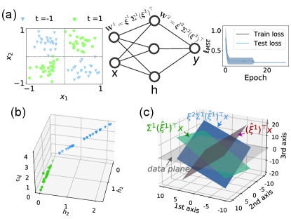
Figure 1:
A simple illustration of the mode decomposition learning.
(a) A deep neural network of three layers, including one hidden layer with three hidden nodes, for a classification task of non-linearly separable data.
The weight matrix , where .
The distribution of input data is modeled as a Gaussian mixture (see the main text) from which
samples are assigned to labels based on the corresponding mixture component.
The training performance is measured by the mean-squared-error loss function .
(b) The representation of hidden neurons plotted in the 3D space, displaying the geometric separation. (c) The successive mappings from
input sample (grey) to (dark red), followed by
(green), and finally
(blue).
A geometric interpretation of Eq. (1) in a simple learning task is shown in Fig. 1. We use a three-layer network with three hidden neurons. The input data is sampled from
a four-component Gaussian mixture Fischer et al. (2022),
(2)
where denotes a Gaussian distribution with mean
and covariances , and .
For the label , , while for ,
. Covariances are isotropic throughout with .
The input samples are
first projected to the input pattern space spanned by ().
Then all three directions of this projection get expanded or contracted via
. Finally the geometrically modified representation is re-mapped to the downstream representation space of a higher dimensionality, as
[Fig. 1 (c)]. The non-linearity of the transfer function is then applied to the last linear transformation, leading to
the geometric separation [Fig. 1 (b)]. We conclude that the MDL provides rich angles to look at the geometric transformation of the input information along the hierarchy of deep networks.
Rather than the conventional weight values in standard backpropagation (BP) algorithms Goodfellow et al. (2016), the trainable
parameters are latent patterns in the MDL.
The training is implemented by stochastic gradient descent in the mode space
SM ,
(3)
where denotes the cost function (e.g., cross-entropy or mean-squared error) over a mini-batch of training data,
denotes the learning rate, and
denotes the error term, which could back-propagate from the top layer where
for (cross entropy). Based on the chain rule, the error backpropagation equation can be derived as
SM .
To ensure the pre-activation is independent of the upstream-layer width, we take the initialization scheme that
Jiang et al. (2021).
To avoid the ambiguity of choosing patterns (e.g., scaled by a factor), we impose an identical regularization with strength
for all trainable parameters. However, our result does not change qualitatively with the specific values of regularization SM .
We remark that for each hidden layer, there exist two types of pattern (). Equation (3) is used to learn these patterns.
We call this case 1L2P. If we assume , the training can be further simplified as in SM , and we call this case 1L1P.
The nature of this mode-based-computation can be understood as an expanded linear-nonlinear layered computation, as
where the linear field
and the equivalent weight . Therefore, the number of
modes acts as the linear-layer width. We leave a systematic exploration of this linear-nonlinear structure by statistical mechanics in forthcoming works.
On-line learning dynamics in a shallow network.—
The MDL can be analytically understood in an on-line learning setting, where we consider one-hidden-layer architecture. The on-line learning can be considered as a special case of
the above mini-batch learning (i.e., the batch size is set to one, and the sample is visited by the learning only once).
The training dataset consists of pairs . Each training example is independently
sampled from a probability distribution , where
is a standard Gaussian distribution, and the scalar label is
generated by the neural network of hidden neurons, (i.e., teacher, indicated by the symbol below).
Given an input , the corresponding label is created by
(4)
where denotes the -th row of
the matrix ,
and represents the -th element of the teacher local field vector
.
The teacher network is quenched as
.
Here, we focus on the non-linear transfer function . In addition,
we train the other shallow network called the student network, by minimizing the loss function
over the training data (labels are given by the teacher network),
where denotes the trainable parameters. The student’s prediction for a fresh sample is given by
(5)
where denotes the -th component of the student local field ,
and the student has hidden neurons. The student is supplied with data samples in sequence (one sample each time step). We next use to indicate the time step as well.
The mean-squared-error can be evaluated as
(6)
where indicates the teacher’s output, and we have replaced the expectation
by ,
because of the central-limit theorem and the i.i.d. setting we consider Biehl and Schwarze (1995); Saad and Solla (1995); Goldt et al. (2019).
The covariance of the local field can be specified as follows,
(7)
where ,
,
and .
By definition, is fixed, while and evolve according to the gradient updates,
following a set of deterministic ordinary differential equations (ODEs) as the input dimension SM . These matrices are exactly the order parameters in physics.
For simplicity, we consider and , i.e., only the upstream patterns are learned.
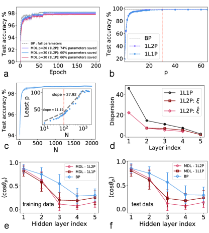
Figure 2: Test performance and mode hierarchy of MDL in deep neural networks.
(a) Training trajectories of a four-layer network, indicated by ---, where each number indicates the
corresponding layer width. The number of modes for layer , where .
, or .
Networks are trained on the full MNIST dataset ( images) and tested on an unseen dataset containing images.
The fluctuation is computed over five independent runs.
(b) Testing accuracy versus (the number of modes is the same for all layers).
The same architecture as (a) is used. The error bar characterizes the fluctuation across
five independently trained networks, and each marker denotes the average result.
The least number of modes is indicated by the dash-dot line.
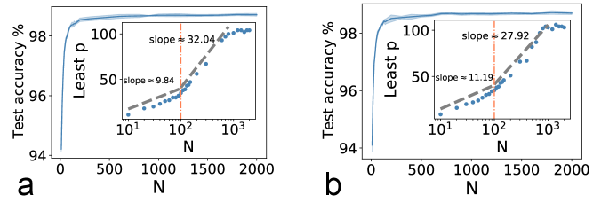
(c) The performance changes with the network width. The inset shows the least number of modes versus the layer width (in the logarithmic scale).
The network architecture is given by ---.
The dash-dot line in the inset separates the piecewise logarithmic increase () regions.
The result is
obtained from five independent runs.
(d) The averaged Euclidean distance (dispersion) from the pattern-cloud center
as a function of layer index.
The network architecture is specified by ---- ().
(e-f) Subspace overlap (principal angle) versus layer. The overlap is averaged with five independent runs, and seven-layer networks with hidden-layer width are trained ().
Results.—
MDL can reach a similar test accuracy with that of BP performed
in the weight space, when is sufficiently large [Fig. 2 (a)].
The computational cost of the BP scales with . In contrast, MDL works in the mode space, requiring a training cost of only the order of
. Note that is much smaller than (or ), and our MDL does not need any additional training constraints (compared to other matrix factorization algorithms SM ).
Remarkably, when , the performance of MDL already matches that of BP [Fig. 2 (b)], but only utilizes of the full sets of parameters that are consumed by the BP.
In fact, each hidden layer can have two different types of latent pattern (1L2P) due to the mode decomposition. But if we assume that
, i.e., each layer share a single type of pattern (1L1P), we can further reduce the computational cost by an amount of , without
sacrificing the test accuracy [Fig. 2 (b)]. Varying the network width, we reveal a logarithmic increase of the least number of modes [Fig. 2 (c)],
which is a novel property of deep learning in the mode space, in stark contrast to a linear number of memory patterns in previous studies Jiang et al. (2021). When the network width further grows,
the least number can even become a constant. We argue that this manifests three separated phases of poor-good-saturated performance with increasing layer width (see Fig. S9 in SM ).
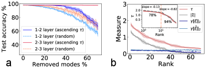
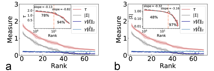
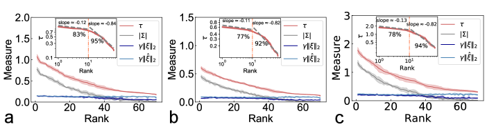
Figure 3: The robustness properties of well-trained four-layer
MDL models with the architecture ---. The case of 1L1P is considered with in the hidden layers.
(a) Effects of removing modes through two protocols: removing modes with weak measure
first (solid line) and removing modes randomly (dashed line).
The fluctuation is computed over ten independent runs.
(b) The rescaled norms , and
the absolute values of versus their rank (in descending order) in
the hidden layers, where
.
The inset shows a log-log plot of the measure, displaying a piecewise power-law behavior.
The error bar is computed over five independent runs. The marked percentage indicates
the generalization accuracy after removing the corresponding side of modes.
To see how the latent patterns are transformed in geometry along the network hierarchy, we first calculate the center of the pattern space.
Then the Euclidean distance from this center to each pattern is analyzed.
We find that the pattern space becomes progressively compact when going to deep layers [Fig. 2 (d)].
To further characterize the geometric details, we define the subspace spanned by the principal eigenvectors of the layer neural responses to one type of inputs.
Then the subspace overlap is calculated as the cosine of the principal angle between two subspaces corresponding to two types of inputs Bjoerck and Golub (1973); SM .
We find that
the hidden-layer representation becomes more disentangled with layer in comparison with BP [Fig. 2 (e,f)].
MDL shows great computational benefits of representation disentanglement, thereby facilitating discrimination. A slight increase of the overlap is observed for deeper layers,
which is caused by the saturation of the test performance (see more analyses in SM ).
Compared to other matrix factorization methods, MDL has no additional constraints for the modes and importance scores, therefore being flexible for feature extraction.
We find that the interlayer patterns are less orthogonal than the intralayer ones. The geometric transformation carried out by
these latent pattern matrices is not strictly a rotation for which the norm is preserved. This flexibility may be the key to make our method better than other matrix factorization
methods in both training cost and learning performance (see details in SM ).
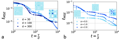
Figure 4: Mean-squared error dynamics in terms of ,
where denotes the on-line sample index, and is the input dimension.
The teacher and student networks share the same number of hidden neurons ().
Markers represent results of the simulation, while the solid lines denote the
theoretical predictions from solving the mean-field ODEs. The number of modes (
denotes the mode load here).
(a) Fixed .
(b) Fixed . The color deepens as or increases. The insets display the evolving matrix for and , respectively.
We next ask whether some modes are more important than the others.
Therefore, we rank the modes according to the
measure ,
where
to make comparable the magnitudes
of the pattern and importance () score.
Removing modes with weak values of first yields much higher accuracy than the random removal protocol [Fig. 3 (a)],
suggesting the existence of leading modes. Moreover, deeper layers are more robust. Figure 3 (b) shows the measure as a function of rank in descending order, which can be
approximately captured by piecewise power-law behavior (a transition point at the rank ). Ranking with only the importance scores yields similar behavior SM .
A small exponent is observed for the leading measures, while the remaining measures bear a large exponent, thereby
revealing the coding hierarchy of latent modes in the deep networks. This intriguing behavior does not change with the regularization strength or the hidden-layer width SM .
Finally, the on-line mean-squared error dynamics of our model can be predicted perfectly in a teacher-student setting.
The number of modes strongly affects the shape of the learning dynamics, and a large mode load can make the plateaus disappear (Fig. 4).
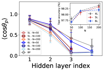
Moreover, during learning, the alignment between receptive fields of the student’s hidden nodes and the teacher’s ones continuously emerge, which is called the specialization transition Schwarze (1993); Goldt et al. (2019).
Conclusion.—
In this Letter, we propose a mode decomposition learning that works in the mode space rather than the conventional weight space.
This learning scheme has three-fold technical and conceptual advances. First, the learning can achieve the comparable performance with standard methods, with a significant reduction of training costs.
We also find that the least number of modes grows only logarithmically with the network width and becomes even independent of larger width, which is in stark contrast to a linear number of patterns in recurrent memory networks.
Second, the learning leads to progressively compact pattern spaces, which promotes highly disentangled hierarchical representations.
The upstream pattern maps the activity into a low-dimensional space, and then the resulting embedding is
further expanded or contracted. After that, the modified embedding is re-mapped into the high-dimensional activity space. This sequence of geometric transformation
can be understood as a linear-nonlinear hidden structure. Third, all modes are not equally important to the generalization ability of the network, showing an intriguing
piecewise power-law behavior. Finally, the mode learning dynamics can be predicted by the mean-field ODEs, revealing the mode specialization transition.
Therefore, the MDL inspires a rethinking of conventional deep learning, offering a faster, more interpretable training framework. Future works along this direction will be inspired.
For example, the impact of other structured dataset, mode dynamics in over-parameterized or recurrent networks, and the origin of adversarial vulnerability of deep networks in terms of geometry of the mode space.
I Acknowledgments
This research was supported by the National Natural Science Foundation of China for
Grant number 12122515, and Guangdong Provincial Key Laboratory of Magnetoelectric Physics and Devices (No. 2022B1212010008), and Guangdong Basic and Applied Basic Research Foundation (Grant No. 2023B1515040023).
Supplemental Material
Appendix A Derivation of learning equations
In this section, we show how to derive the updating equations for
the mode parameters where
the superscript indicates the layer index in the range from to . The loss function
is the cross entropy averaged over all training examples (divided into mini-batches in stochastic gradient descent),
where is defined as the target label (one-hot representation as common in machine learning).
After training the network on the training dataset with size , we evaluate the generalization
performance of the network on the unseen dataset with size .
In our framework of mode decomposition learning, the weight is decomposed into the form as follows,
(S1)
The mode parameters are updated according to gradient descent of the loss function,
(S2)
where denotes the learning rate, and the error propagation term
. On the top layer, can be computed with
the result . For lower layers, the term can be iteratively computed
using the chain rule. More precisely,
(S3)
The explicit expressions of gradient steps for the three sets of mode parameters are given as follows,
(S4)
The above learning equations apply to the case of 1L2P case.
Next, we consider the 1L1P case ().
Apart from the single input pattern for the first layer and the single output pattern for
the last layer , two types of pattern in each hidden layer take
the same form, and we denote .
The expression of remains unchanged, and we can then update
according to Eq. (S4). Next, we give the gradient descent equation for where as follows
(S5)
where two terms contribute to the gradient—the first one comes from the contribution of ,
while the second one originates from the fact that the same pattern can act as .
To ensure the weighted sum in the pre-activation is independent
of the upstream layer width and the number of modes , we choose the initialization scheme such that
. This scaling is inspired by
studies of Hopfield models Jiang et al. (2021).
In practice, we independently and identically sample the initial elements
from the standard Gaussian distribution, and then the weight values are multiplied by a factor of .
Note that the number of modes are assumed to be proportional to . But if the number is a constant denoted by , then the factor could
be .
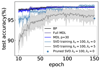
Figure S1: The comparison among the SVD training, MDL (1L2P) and traditional BP in learning performance.
The network structure is specified by in all cases. The full MDL indicates the MDL with the same number of parameters as that of the SVD training,
while the blue dot (pruned SVD) indicates the pruning of the full SVD model (the modes with small ranked in descending order) modes off each layer (except the output layer) to make the consuming parameter amount
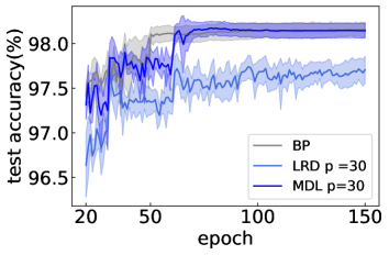
comparable with that of MDL with .Figure S2: The comparison among low-rank decomposition (LRD), MDL (1L2P) and traditional BP.
Both decomposition methods use . The network structure is in all cases.
Appendix B Comparison to other matrix factorization methods
Here, we compared our MDL method to other matrix factorization methods in learning performance. These other methods include singular value decomposition (SVD),
low rank decomposition (LRD) and spectral training Yang et al. (2020); Chicchi et al. (2021).
First, the SVD learning scheme is implemented by decomposing the weight of each layer as
(S6)
where the diagonal matrix contains non-zero elements in the diagonal, and the elements of is constrained to be positive.
The orthogonality is forced by two regularization terms as
(S7)
where is the original training loss, ,
and .
is the rank of and , denotes the Frobenius norm of a matrix.
The regularization term forces and to be orthogonal, while adjusts the sparsity level of .
The gradients for each set of parameters are derived below,
(S8)
For comparison, we carried out the SVD learning, with , , and , , as shown in Fig. S1.
We remark that the training cost is larger for SVD models,
which can be calculated as . Taking as
an example, the learning needs parameters in total. However, for our MDL with which already reaches the traditional BP performance,
the learning only needs parameters (but traditional BP needs parameters).
In simulations, we prune the full SVD model ((the modes with small ranked in descending order)) modes off each layer (except the output layer) to make the number of trainable parameters comparable with that of
MDL with . We conclude that the MDL consumes less parameters, yet produces rapid learning with even better performances.
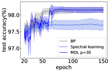
Figure S3: The comparison among the spectral learning, MDL (1L2P) and traditional BP. The network structure is in all cases.
Next, we fix in our MDL, and this reduced form is called the low rank decomposition as follows,
(S9)
In the simulation, we set . We can see in Fig. S2 that the performance of the LRD is much worse than that of MDL and traditional BP.
For the recently proposed spectral learning Chicchi et al. (2021), a carefully-designed transformation matrix (an matrix, is the total number of units in the network, and
is a layer index) is used with a spectral decomposition. The eigenvalues and the associated basis are optimized. However, this training performs worse compared to our MDL in the examples shown in Fig. S3.
Appendix C Ranking the modes according to the importance matrix
Here, we rank the modes according to the diagonal of the importance matrix, rather than the measure. We found that these two ranking schemes lead to qualitatively identical results.
Removing the most important modes (according to either the measure or the importance score) will significantly impair the generalization ability of the network.
Details are illustrated in Fig. S4. The non-smooth behavior can be attributed to the existence of mode-contribution gap, i.e., the most important modes ( for the measure; for
the measure) dominate the generalization capability of the network, while other modes capture irrelevant noise in the data.
Figure S4: Ranking modes. The network structure is , and we analyze the 1L1P case here with .
The marked percentage in the inset indicates the generalization accuracy after removing the corresponding side of modes in the hidden layer.
The piecewise power law behavior is retained for both types of ranking.
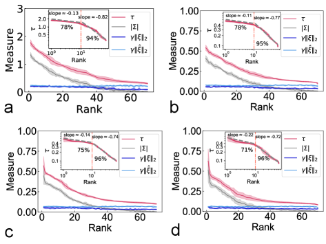
Appendix D The qualitative behavior of the MDL does not change with the regularization strength or the hidden-layer width
Further, our MDL is in essence a matrix factorization. Therefore, the pattern and importance matrices are not unique. However, in practice, we impose the norm level for these patterns and importance scores.
In fact, we find the intriguing properties of the MDL in deep learning do not change with the regularization strength of the norm (denoted as , see Fig. S8). Figure S5 shows an example
for the behavior of the optimal number of modes versus hidden-layer width, while Fig. S6 shows that the piecewise power law behavior of the measure does not change with the regularization strength.
In addition, the piecewise power law behavior of the measure does not change with the hidden-layer width as well (Fig. S7).
Figure S5: The piecewise increasing behavior of the least with the hidden-layer width.
The network has structure , and we vary to get the corresponding least ,
which is defined as the least number of modes that MDL needs to reach the performance of the traditional BP. 1L2P case is considered.
(a) and (b) are obtained under different regularization strengths. (a) . (b) . Figure S6: The piecewise power law behavior of the measure does not change with the regularization strength in the 1L1P case.
The network structure is specified by . (a) . (b) . (c) .Figure S7: The piecewise power law behavior of the measure does not change with the hidden-layer width in the 1L1P case. The network structure is specified by .
(a) . (b) . (c) . (d) .
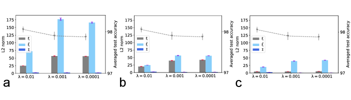
Figure S8: The norm of parameters under three regularization strengths— . The network structure is specified by and for all layers, where the 1L1P case is considered (the 1L2P case yields
qualitatively the same results). (a, b, c) are plotted for the first layer, the second layer, and the output layer, respectively.
Appendix E Subspace overlap of layered response to pairs of stimuli
In this section, we provide details of estimating the average degree of correlation between neural
responses to pairs of different input stimuli (e.g., one stimulus contains images of the same class). The covariance of neural response in each layer to the stimulus can be diagonalized to specify a low-dimensional subspace.
The subspace is spanned by the first principal components. The subspace
overlap can then be evaluated via the cosine of the principal angle between these two subspaces corresponding to two different stimuli.
In practice, for neural responses in each layer
to the stimulus (e.g., many images of digit ), we first identify the first principal
components of the covariance of , which explains over of the total variance, and then reorganize the eigenvectors to
an matrix, namely . We repeat this procedure for another stimulus , and get another matrix .
Therefore, the columns of and span two subspaces corresponding to the neural
responses to and respectively. The cosine of the principal angle between these two subspaces is calculated as follows Bjoerck and Golub (1973)
(S10)
where denotes the largest singular value of the matrix .
In simulations, we consider the classification task of the MNIST dataset, where ten classes of digits are fed into
a seven-layer neural network. Specifically, we choose that can explain over of the total variance for each
stimulus and each layer, and therefore the value of varies with layer and input stimulus.
In the main text, we observe a mild increase of the subspace overlap in deep layers. Here, as shown in Fig. S9, we link this behavior to the saturation of the test performance with increasing number of layers and network width.
In addition, the task we consider is relatively simple, and thus three hidden layers (five layers in total) are sufficient to classify the digits with a high accuracy.
The subspace overlap under the MDL setting thus suggests a consistent way to determine the optimal number of layers and the network width in practical training.
Figure S9: The averaged subspace overlap versus layers. Different number of layers with different hidden-layer widths are considered. The results are averaged over five independent trainings. The inset
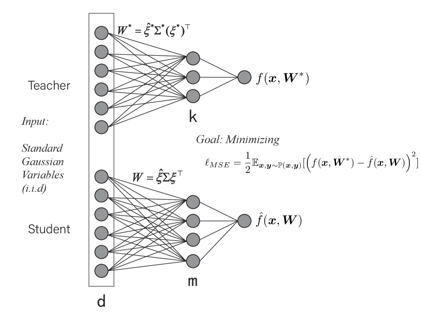
shows the corresponding test accuracy changing with the hidden-layer width.Figure S10: A simple illustration of the teacher-student setup
with i.i.d. standard Gaussian input. The teacher network has
hidden nodes and modes, while the student network has hidden nodes and modes.
The goal of the student network is to predict the labels generated by
the teacher network, minimizing the mean-squared error. The weights to the output layer are set to
one in the linear readout for both teacher and student networks (, and is an all-one vector of length ).
Appendix F Mean-field predictions of on-line learning dynamics
In this section, we give a detailed derivation of the mean-field ordinary differential equations for
the on-line dynamics. A sketch of the toy model setting is shown in Fig. S10. The label for each sample (i.i.d. standard
Gaussian variable) is generated by the teacher network,
(S11)
where
denotes the -th row of the matrix ,
and
represents the -th element of the teacher local field vector .
To ensure the local field is independent of the input dimension,
we choose the initialization scheme for the teacher network
such that .
More precisely, we set the elements to be independent standard
Gaussian variables, and then multiply the weight values by a factor of for logarithmic increasing number of modes.
This scaling ensures that the magnitude of the weight values is of the order one.
Different
forms of transfer function can be considered, but we choose the error function for the simplicity of the following theoretical analysis.
The prediction of the label by the student
network for a new sample is given by
(S12)
where denotes the -th
component of the student local field
.
The student network has hidden nodes and patterns. For simplicity, we assume , , and only the pattern is learned.
Training the student network with the one-pass gradient descent (on-line learning) directly minimizes the following mean-squared error (MSE):
(S13)
where indicates the average over that can be replaced by the average over local fields.
For the Gaussian data ,
the dynamics of can be completely determined by the following order parameters: ,
,
and .
The corresponding matrix elements are denoted as , and . Then we can define the local-field covariance
matrix at time step as follows,
(S14)
where is fixed by definition (parameters of the teacher network are quenched), the sample index is also the time step in the on-line learning setting,
and the evolution of other order parameters and is driven by the gradient flow
of the mode parameters . The loss is
completely determined by the evolving order parameters,
(S15)
where
(S16)
To proceed, we define the integral
, which
has an analytic form for as follows,
(S17)
where denotes the element of the overlap matrix for and , in which
and indicate the attributes of the network—teacher or student.
Therefore, the generalization error can be estimated as follows,
(S18)
We next consider the evolution of the order parameters, which involves only the update of in our toy model setting.
Therefore, we derive the evolution of order parameters and
based on the gradient of : .
In the high-dimensional limit (), we use the self-averaging property of the order parameters considering the disorder average over the input data distribution Biehl and Schwarze (1995); Saad and Solla (1995); Goldt et al. (2019).
Then we have the following expressions,
(S19)
where the expectation is carried out with respect to the data distribution.
Inserting the update equation of into the equation of the order parameter , we get
(S20)
where we have applied the definition of to derive the second equality.
Considering the definition of , ,
, and , we recast Eq. (S20) as follows,
(S21)
To proceed, we have to estimate the integral defined by
for our transfer function , where
denotes the element of the field-covariance matrix
. We also have to estimate the second integral defined by
, which has a closed form as
(S22)
where
(S23)
In an analogous way, we can derive the mean-field evolution of as follows,
(S24)
where the definition of has bee used.
If we define , and take the thermodynamic limit of , the time step becomes continuous, and we can thus write down the following ODEs,
(S25)
where the index in or with the symbol labels the teacher’s local-field.
References
Goodfellow et al. (2016)
I. Goodfellow,
Y. Bengio, and
A. Courville,
Deep Learning (MIT Press,
Cambridge, MA, 2016).
Carleo et al. (2019)
G. Carleo,
I. Cirac,
K. Cranmer,
L. Daudet,
M. Schuld,
N. Tishby,
L. Vogt-Maranto,
and
L. Zdeborová,
Rev. Mod. Phys. 91,
045002 (2019).
Huang (2022)
H. Huang,
Statistical Mechanics of Neural Networks
(Springer, Singapore,
2022).
Roberts et al. (2022)
D. A. Roberts,
S. Yaida, and
B. Hanin,
The Principles of Deep Learning Theory: An Effective
Theory Approach to Understanding Neural Networks
(Cambridge University Press,
Cambridge, 2022).
Jaderberg et al. (2014)
M. Jaderberg,
A. Vedaldi, and
A. Zisserman,
arXiv:1405.3866 (2014).
Yang et al. (2020)
H. Yang,
M. Tang,
W. Wen,
F. Yan,
D. Hu,
A. Li,
H. Li, and
Y. Chen,
2020 IEEE/CVF Conference on Computer Vision and Pattern
Recognition Workshops (CVPRW) (2020).
Giambagli et al. (2021)
L. Giambagli,
L. Buffoni,
T. Carletti,
W. Nocentini,
and D. Fanelli,
Nature Communications 12,
1330 (2021).
Chicchi et al. (2021)
L. Chicchi,
L. Giambagli,
L. Buffoni,
T. Carletti,
M. Ciavarella,
and D. Fanelli,
Phys. Rev. E 104,
054312 (2021).
Jiang et al. (2021)
Z. Jiang,
J. Zhou,
T. Hou,
K. Y. M. Wong,
and H. Huang,
Phys. Rev. E 104,
064306 (2021).
Zhou et al. (2021)
J. Zhou,
Z. Jiang,
T. Hou,
Z. Chen,
K. Y. M. Wong,
and H. Huang,
Phys. Rev. E 104,
064307 (2021).
(11)
Y. LeCun, The MNIST database of handwritten digits, retrieved
from http://yann.lecun.com/exdb/mnist.
Fischer et al. (2022)
K. Fischer,
A. Ren’e,
C. Keup,
M. Layer,
D. Dahmen, and
M. Helias,
arXiv:2202.04925 (2022).
(13)
See the supplemental material at http://… for technical and
experimental details.
Biehl and Schwarze (1995)
M. Biehl and
H. Schwarze,
Journal of Physics A: Mathematical and General
28, 643 (1995).
Saad and Solla (1995)
D. Saad and
S. A. Solla,
Phys. Rev. Lett. 74,
4337 (1995).
Goldt et al. (2019)
S. Goldt,
M. S. Advani,
A. M. Saxe,
F. Krzakala, and
L. Zdeborová,
arXiv:1901.09085 (2019).
Bjoerck and Golub (1973)
A. Bjoerck and
G. H. Golub,
Mathematics of Computation 27,
579 (1973).
Schwarze (1993)
H. Schwarze,
J. Phys. A: Math. Gen. 26,
5781 (1993).