Emergence of multiphoton quantum coherence by light propagation
Abstract
The modification of the quantum properties of coherence of photons through their interaction with matter lies at the heart of the quantum theory of light. Indeed, the absorption and emission of photons by atoms can lead to different kinds of light with characteristic quantum statistical properties. As such, different types of light are typically associated with distinct sources. Here, we report on the observation of the modification of quantum coherence of multiphoton systems in free space. This surprising effect is produced by the scattering of thermal multiphoton wavepackets upon propagation. The modification of the excitation mode of a photonic system and its associated quantum fluctuations result in the formation of different light fields with distinct quantum coherence properties. Remarkably, we show that these processes of scattering can lead to multiphoton systems with sub-shot-noise quantum properties. Our observations are validated through the nonclassical formulation of the emblematic van Cittert-Zernike theorem. We believe that the possibility of producing quantum systems with modified properties of coherence, through linear propagation, can have dramatic implications for diverse quantum technologies.
I Introduction
The description of the evolution of spatial, temporal, and polarization properties of the light field gave birth to the classical theory of optical coherence [1, 2, 3, 4, 5, 6, 7]. Naturally, these properties of light can be fully characterized through the classical electromagnetic theory [3]. Furthermore, there has been interest in describing the evolution of propagating quantum optical fields endowed with these classical properties [8, 9]. This has been accomplished by virtue of the Wolf equation and the van Cittert-Zernike theorem [1, 8, 10, 11]. Nevertheless, there is a long-sought goal in describing the evolution of the inherent quantum mechanical properties of the light field that define its nature and kind [12, 13]. Such formalism would enable modeling the evolution of the excitation mode of propagating electromagnetic fields in the Fock number basis. Given the large number of scattering and interference processes that can take place in a quantum optical system with many photons, this ambitious description remains elusive [14, 15, 16, 17, 18]. Although, it is essential to describe the evolution of propagating multiphoton wavepackets in diverse quantum photonic devices [18, 19, 20, 21].
The quantum theory of optical coherence developed by Glauber and Sudarshan provides a description of the excitation mode of the electromagnetic field [13, 12, 22]. This elegant formalism led to the identification of different kinds of light that are characterized by distinct quantum statistical fluctuations and noise levels [15, 23, 12, 22, 24]. As such, a particular quantum state of light is typically associated with a specific emission process and a light source [22]. Moreover, the quantum theory of electromagnetic radiation enables describing light-matter interactions [25]. These consist of absorption and emission processes that can lead to the modification of the excitation mode of the light field and consequently to different kinds of light [25, 22]. This possibility has triggered interest in achieving optical non-linearities at the single-photon level to engineer and control quantum states of light [26, 27, 28, 29]. Thus, it is believed that the excitation mode of the light field, and its quantum properties of coherence, remain unchanged upon propagation in free space [22, 25].
We demonstrate that the statistical fluctuations of thermal light fields, and their quantum properties of coherence, can be modified upon propagation in the absence of light-matter interactions [9, 33]. This effect results from the scattering of multiphoton wavepackets that propagate in free space. The large number of interference effects hosted by multiphoton systems with up to twenty particles leads to a modified light field with evolving quantum statistical properties [16, 14]. Further, we show that the evolution of multiphoton quantum coherence can be described by the nonclassical formulation of the van Cittert-Zernike theorem [9]. Interestingly, our description of propagating multiphoton quantum coherence unveils conditions under which multiphoton systems with sub-shot-noise quantum properties are formed [34]. Remarkably, these quantum multiphoton systems are produced upon propagation in the absence of optical nonlinearities [26, 27, 28, 29]. As such, we believe that our findings provide an all-optical alternative for the preparation of multiphoton systems with nonclassical statistics. Given the relevance of photonic quantum control for multiple quantum technologies, similar functionalities have been explored in nonlinear optical systems, photonic lattices, plasmonic systems, and Bose-Einstein condensates [35, 17, 36, 26, 27, 28, 29].
II Experiment and Results Discussion
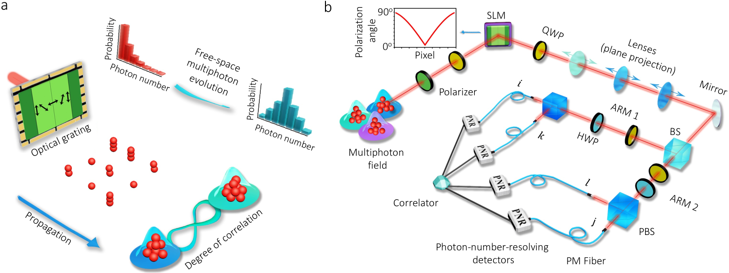
The optical system under consideration is depicted in Figure 1a. In this case, an unpolarized thermal field is scattered by an optical grating to produce multiphoton wavepackets with distinct polarization properties at different transverse spatial positions [5]. The scattered photons contained in the thermal beam interfere upon propagation to change the statistical fluctuations of the field [9]. Interestingly, these effects enable the modification of the quantum properties of coherence of the initial multiphoton thermal system in free space. As discussed in the Supplementary Information (SI), we describe our initial thermal system as an incoherent superposition of coherent states [13, 12, 37]
| (1) |
where represents a coherent state of amplitude with random mode-structure , where and polarization (see SI). Furthermore, the tensor product over positions represents the pixelated transverse beam profile where each pixel has sidelength .
After the polarization grating, the resulting state is obtained via the transformation
| (2) |
where is the mode for photon loss and are the components of the transformation
| (3) |
where and is the length of the polarization grating. The beam described by Eq. (1) is then propagated by a distance of before being measured by two pairs of photon-number-resolving (PNR) detectors [23, 38]. This propagation can be modeled through the Fresnel approximation on the mode structure of the initial beam [39]. We can then compute the second-order correlation function
for the post-selected polarization measurements in the detection plane as [2]
| (4) | ||||
Remarkably, the Dirac-delta functions in Eq. (4) demonstrate the presence of nontrivial correlations. Given the complexity of and , their explicit expressions are given in the SI. These describe the coherence of a photon with itself, which existed prior to interacting with the grating, and the spatial coherence gained by multiphoton scattering. These terms unveil the possibility of modifying quantum coherence of multiphoton systems upon propagation [9]. We use this approach to describe the correlation properties of the multiphoton wavepackets that constitute our light beam. This allows us to use an equivalent density matrix for the system (see SI) at the detection plane to compute its corresponding joint photon-number distribution as
| (5) |
As we shall see in the next section, these formulae allow for the prediction of very interesting correlation effects. Specifically, they predict that the statistical make-up of the light field is changing upon propagation in free space. The classical analogue to this behavior is explained by the van Cittert-Zernike theorem [10, 11], which predicts that the classical coherence properties of a light source can change upon free-space propagation. Therefore, we interpret our results in Eq. (4) as those of a quantum van Cittert-Zernike theorem. This is because they predict the modification of quantum coherence upon free-space propagation, and that is directly analogous to the classical theorem’s predictions. Specifically, Eq. (4) predicts this free-space quantum modification through the nontrivial scattering effects induced by the Dirac-delta functions. Interestingly, these delta functions arise from the unique coherence properties of thermal light (see SI for further details). Furthermore, Eq. (5) allows us to study multiparticle quantum coherence, which is also changing upon free-space propagation. These quantum van Cittert-Zernike effects, therefore, are not only arising in polarization subsystems, but also in multiphoton subsystems. This showcases the fundamental and intrinsic quantum impacts of free-space propagation on our state.
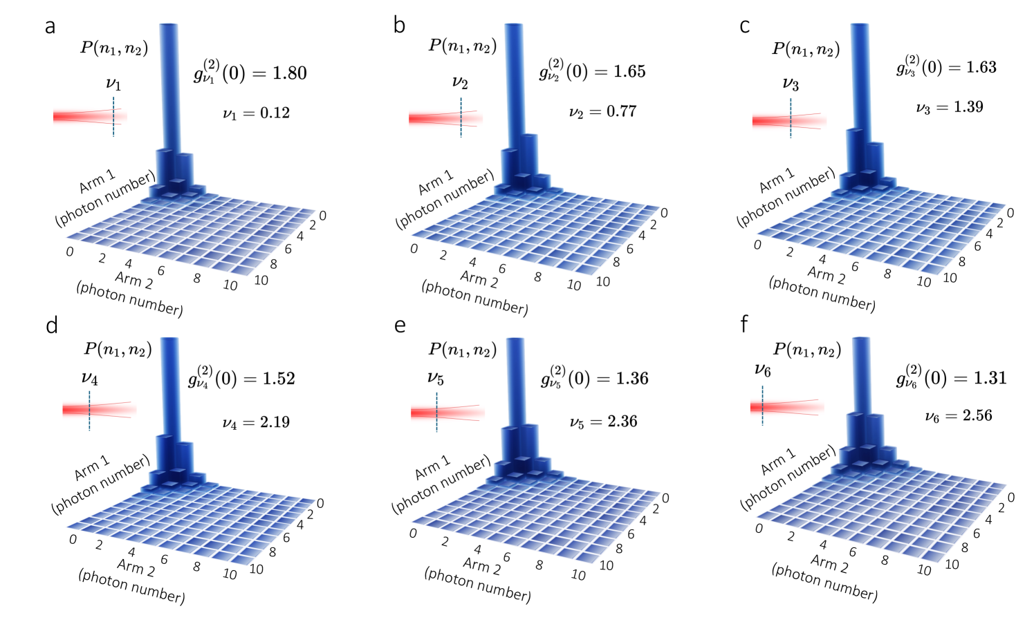
We explore the modification of the quantum coherence properties of propagating multiphoton systems using the experimental setup in Figure 1b. We use a combination of waveplates and a spatial light modulator (SLM) to rotate the polarization properties of our multiphoton system at any transverse position [30]. In addition, this arrangement enables us to characterize the polarization and photon-number distribution of multiphoton systems at different propagation planes. Specifically, we perform measurements at different propagation planes associated with the propagation parameter . Here, the transverse distance between detectors is described by and the wavelength of the beam by . As demonstrated in Figure 2, the many interference effects hosted by the propagating multiphoton system modify the photon-number distribution of the polarized components of the initial beam [15, 17, 20]. These processes lead to multiphoton systems with different quantum fluctuations and quantum properties of coherence [15, 40]. Each multiphoton system is characterized through the degree of second-order self coherence
| (6) |
where . Interestingly, the multiphoton system in Figure 2a is nearly thermal [22]. However, propagation leads to different kinds of multiphoton wavepackets. We show these from Figure 2a to f. The coherence properties of the multiphoton system in Figure 2f approach those observed in coherent light beams [34]. Remarkably, the conversion processes of the multiphoton system, described by Eq. (5), take place in free space in the absence of light-matter interactions [25, 26, 27, 28, 35, 17, 36].
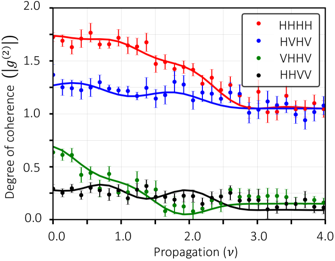
The polarization and photon-number properties of the propagating light beam at different transverse and longitudinal positions host many forms of interference effects [37, 14]. We explore these dynamics by isolating the constituent multiphoton subsystems of the propagating beam. Each multiphoton subsystem, characterized by different polarization properties, exhibits different degrees of second-order coherence [20]. In the experiment, we perform projective measurements on polarization. These measurements unveil the possibility of extracting multiphoton subsystems with attenuated quantum fluctuations below the shot-noise limit [38, 32]. In this case, we use the four detectors depicted in the experimental setup in Figure 1b to perform full characterization of polarization [31]. These measurements enable us to characterize correlations of multiphoton subsystems with different polarization properties, which are reported in Figure 3. We plot the degree of second-order mutual coherence
| (7) |
The propagation of the multiphoton subsystem described by shows a modification of the quantum statistics from super-Poissonian to nearly Poissonian [40, 34]. A similar situation prevails for the multiphoton subsystem described by . It is worth noticing that the multiphoton subsystems described by and unveil the possibility of extracting multiphoton subsystems with sub-shot-noise properties [41]. This implies photon-number distributions narrower than the characteristic Poissonian distribution of coherent light [22, 42]. This peculiar feature might unlock novel paths towards the implementation of sensitive measurements with sub-shot-noise fluctuations [43].
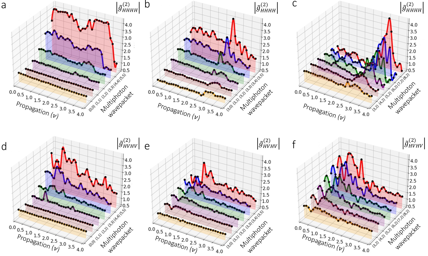
We now turn our attention to describe the quantum coherence evolution of propagating multiphoton wavepackets. This is explored by projecting the polarized components of the initial thermal beam into its constituent multiphoton wavepackets [22]. In this case, we analyze wavepackets with number of photons. The number of photons detected in arm 1 of our experiment is described by , whereas indicates the number of photons detected in arm 2. Our findings unveil that despite the fact that the degree of second-order coherence in Figure 3 is produced by its constituent wavepackets, these show a completely different evolution of their properties of coherence. Our experimental measurements of these wavepackets can be found from Figure 4a to c. The results in Figure 4a indicate that multiphoton wavepackets, in which and are the same, show a particular evolution. In contrast, propagating wavepackets with asymmetric values of and show different trends in the modification of quantum coherence, these are shown in Figure 4b and c. The propagation of these wavepackets can be described using Eq. (5). Specifically, we can calculate the multiphoton degree of second-order mutual coherence [44]
| (8) |
Furthermore, the multiphoton wavepackets in the projected beam, characterized by , exhibit the multiphoton dynamics reported from Figure 4d to f. These results suggest that the multiphoton dynamics in Figure 4 depend on the number of photons in each of the measured wavepackets.
This quantum field theoretic approach to studying the quantum van Cittert-Zernike theorem provides us with the ability to describe the propagation dynamics of the multiphoton systems that constitute classical light beams. We used this formalism to extract propagating multiphoton subsystems, with quantum statistical properties, from unpolarized thermal light fields. While nonlinear light-matter interactions offer the possibility of engineering complex quantum systems [26, 27, 28], our scheme exploits linear propagation of multiphoton systems [29, 45]. This feature enabled us to exploit multiphoton scattering in free space to produce wavepackets with different quantum statistical properties [15]. As such, our work combines the benefits of post-selective measurements with those of multiphoton scattering in propagating light beams, and it allows us to study the modification of the quantum statistical properties of multiphoton wavepackets in free space. Although, the incoherent combination of light beams with different polarization properties can lead to the modification of the degree of second-order coherence [17, 46], we performed direct measurements of polarized multiphoton systems with propagating quantum coherence properties (see Fig. 4a to c). Interestingly, these processes are defined by the number of particles in the measured multiphoton system. Consequently, these findings have important implications for all-optical engineering of multiphoton quantum systems.
III Conclusion
We demonstrated the possibility of modifying the excitation mode of thermal multiphoton fields through free space propagation. This modification stems from the scattering of multiphoton wavepackets in the absence of light-matter interactions [25, 26, 27, 28, 35, 17, 36, 47]. The modification of the excitation mode of a photonic system and its associated quantum fluctuations result in the formation of different light fields with distinct quantum coherence properties [22, 12, 13]. The evolution of multiphoton quantum coherence is described through the nonclassical formulation of the van Cittert-Zernike theorem, unveiling conditions for the formation of multiphoton systems with attenuated quantum fluctuations below the sub-shot-noise limit [38, 48, 43]. Notably, these quantum multiphoton systems emerge in the absence of optical nonlinearities, suggesting an all-optical approach for extracting multiphoton wavepackets with nonclassical statistics. We believe that the identification of this surprising multiphoton dynamics has important implications for multiphoton protocols quantum information [18, 21].
Acknowledgments
J.F. acknowledges funding from the National Science Foundation through Grant No. OMA 2231387. M.H., R.B.D., C.Y. and O.S.M.L. acknowledge support from the Army Research Office (ARO), through the Early Career Program (ECP) under the grant no. W911NF-22-1-0088. R.J.L.-M. thankfully acknowledges financial support by DGAPA-UNAM under the project UNAM-PAPIIT IN101623.
References
References
- Wolf [1954] E. Wolf, Optics in terms of observable quantities, Il Nuovo Cimento (1943-1954) 12, 884 (1954).
- Mandel and Wolf [1995] L. Mandel and E. Wolf, Optical coherence and quantum optics (Cambridge university press, 1995).
- Born and Wolf [2013] M. Born and E. Wolf, Principles of optics: electromagnetic theory of propagation, interference and diffraction of light (Elsevier, 2013).
- Dorrer [2004] C. Dorrer, Temporal van Cittert-Zernike theorem and its application to the measurement of chromatic dispersion, J. Opt. Soc. Am. B 21, 1417–1423 (2004).
- Gori et al. [2000] F. Gori, M. Santarsiero, R. Borghi, and G. Piquero, Use of the van Cittert–Zernike theorem for partially polarized sources, Opt. Lett. 25, 1291–1293 (2000).
- Zhang et al. [2020] Y. Zhang, Y. Cai, and G. Gbur, Partially coherent vortex beams of arbitrary radial order and a van Cittert–Zernike theorem for vortices, Phys. Rev. A 101, 043812 (2020).
- Cai et al. [2012] Y. Cai, Y. Dong, and B. Hoenders, Interdependence between the temporal and spatial longitudinal and transverse degrees of partial coherence and a generalization of the van Cittert-Zernike theorem, J. Opt. Soc. Am. A 29, 2542–2551 (2012).
- Saleh et al. [2005] B. E. A. Saleh, M. C. Teich, and A. V. Sergienko, Wolf equations for two-photon light, Phys. Rev. Lett. 94, 223601 (2005).
- You et al. [2023] C. You, A. Miller, R. d. J. León-Montiel, and O. S. Magaña-Loaiza, Multiphoton quantum van cittert-zernike theorem, npj Quantum Inf. 9, 50 (2023).
- van Cittert [1934] P. van Cittert, Die wahrscheinliche schwingungsverteilung in einer von einer lichtquelle direkt oder mittels einer linse beleuchteten ebene, Physica 1, 201–210 (1934).
- Zernike [1938] F. Zernike, The concept of degree of coherence and its application to optical problems, Physica 5, 785–795 (1938).
- Glauber [1963a] R. J. Glauber, The quantum theory of optical coherence, Phys. Rev. 130, 2529 (1963a).
- Sudarshan [1963] E. C. G. Sudarshan, Equivalence of semiclassical and quantum mechanical descriptions of statistical light beams, Phys. Rev. Lett. 10, 277 (1963).
- Dell’Anno et al. [2006] F. Dell’Anno, S. D. Siena, and F. Illuminati, Multiphoton quantum optics and quantum state engineering, Phys. Rep. 428, 53 (2006).
- Magaña Loaiza and et al. [2019] O. S. Magaña Loaiza and et al., Multiphoton quantum-state engineering using conditional measurements, npj Quantum Inf. 5, 80 (2019).
- You et al. [2020] C. You, A. C. Nellikka, I. D. Leon, and O. S. Magaña-Loaiza, Multiparticle quantum plasmonics, Nanophotonics 9, 1243–1269 (2020).
- You and et al. [2021a] C. You and et al., Observation of the modification of quantum statistics of plasmonic systems, Nat. Commun. 12, 5161 (2021a).
- Walmsley [2023] I. Walmsley, Light in quantum computing and simulation: perspective, Optica Quantum 1, 35 (2023).
- Magaña-Loaiza and Boyd [2019] O. S. Magaña-Loaiza and R. W. Boyd, Quantum imaging and information, Rep. Prog. Phys. 82, 124401 (2019).
- Bhusal and et al. [2022] N. Bhusal and et al., Smart quantum statistical imaging beyond the Abbe-Rayleigh criterion, npj Quantum Inf. 8, 83 (2022).
- Aspuru-Guzik and Walther [2012] A. Aspuru-Guzik and P. Walther, Photonic quantum simulators, Nat. Phys. 8, 285–291 (2012).
- Glauber [1963b] R. J. Glauber, Coherent and incoherent states of the radiation field, Phys. Rev. 131, 2766 (1963b).
- You and et al. [2020] C. You and et al., Identification of light sources using machine learning, Appl. Phys. Rev. 7, 021404 (2020).
- Kong et al. [2024] L.-D. Kong, T.-Z. Zhang, X.-Y. Liu, H. Li, Z. Wang, X.-M. Xie, and L.-X. You, Large-inductance superconducting microstrip photon detector enabling 10 photon-number resolution, Advanced Photonics 6, 016004 (2024).
- Allen and Eberly [1987] L. Allen and J. H. Eberly, Optical resonance and two-level atoms, Vol. 28 (Courier Corporation, 1987).
- Venkataraman et al. [2013] V. Venkataraman, K. Saha, and A. L. Gaeta, Phase modulation at the few-photon level for weak-nonlinearity-based quantum computing, Nat. Photonics 7, 138–141 (2013).
- Zasedatelev et al. [2021] A. V. Zasedatelev, A. V. Baranikov, D. Sannikov, D. Urbonas, F. Scafirimuto, V. Y. Shishkov, E. S. Andrianov, Y. E. Lozovik, U. Scherf, T. Stöferle, R. F. Mahrt, and P. G. Lagoudakis, Single-photon nonlinearity at room temperature, Nature 597, 493 (2021).
- Snijders et al. [2016] H. Snijders, J. A. Frey, J. Norman, M. P. Bakker, E. C. Langman, A. Gossard, J. E. Bowers, M. P. van Exter, D. Bouwmeester, and W. Löffler, Purification of a single-photon nonlinearity, Nat. Commun. 7, 12578 (2016).
- Hallaji et al. [2017] M. Hallaji, A. Feizpour, G. Dmochowski, J. Sinclair, and A. M. Steinberg, Weak-value amplification of the nonlinear effect of a single photon, Nature Physics 13, 540 (2017).
- Mirhosseini et al. [2014] M. Mirhosseini, O. S. Magaña Loaiza, S. M. Hashemi Rafsanjani, and R. W. Boyd, Compressive direct measurement of the quantum wave function, Phys. Rev. Lett. 113, 090402 (2014).
- Altepeter et al. [2005] J. Altepeter, E. Jeffrey, and P. Kwiat, Photonic state tomography, Adv. At. Mol. Opt. Phys. 52, 105 (2005).
- Hashemi Rafsanjani et al. [2017] S. M. Hashemi Rafsanjani, M. Mirhosseini, O. S. Magana-Loaiza, B. T. Gard, R. Birrittella, B. E. Koltenbah, C. G. Parazzoli, B. A. Capron, C. C. Gerry, J. P. Dowling, and R. W. Boyd, Quantum-enhanced interferometry with weak thermal light, Optica 4, 487 (2017).
- Hong et al. [2024a] M. Hong, D. Riley B., B. Bertoni, C. You, and O. S. Magaña-Loaiza, Nonclassical near-field dynamics of surface plasmons, Nat. Phys. 12, 10.1038/s41567-024-02426-y (2024a).
- Gerry et al. [2005] C. Gerry, P. Knight, and P. L. Knight, Introductory quantum optics (Cambridge university press, 2005).
- Olsen et al. [2002] M. Olsen, L. Plimak, and A. Khoury, Dynamical quantum statistical effects in optical parametric processes, Opt. Commun. 201, 373–380 (2002).
- Kondakci et al. [2015] H. E. Kondakci, A. F. Abouraddy, and B. E. A. Saleh, A photonic thermalization gap in disordered lattices, Nat. Phys. 11, 930 (2015).
- Ou [2007] Z.-Y. J. Ou, Multi-photon quantum interference, Vol. 43 (Springer, 2007).
- You and et al. [2021b] C. You and et al., Scalable multiphoton quantum metrology with neither pre- nor post-selected measurements, Appl. Phys. Rev. 8, 041406 (2021b).
- Goodman [2008] J. W. Goodman, Introduction to Fourier optics (2008).
- Hong et al. [2023] M. Hong, A. Miller, R. d. J. León-Montiel, C. You, and O. S. Magaña-Loaiza, Engineering super-poissonian photon statistics of spatial light modes, Laser Photonics Rev. 17, 2300117 (2023).
- Agarwal [2012] G. S. Agarwal, Quantum optics (Cambridge University Press, 2012).
- Mandel [1979] L. Mandel, Sub-poissonian photon statistics in resonance fluorescence, Opt. Lett. 4, 205–207 (1979).
- Lawrie et al. [2019] B. J. Lawrie, P. D. Lett, A. M. Marino, and R. C. Pooser, Quantum sensing with squeezed light, ACS Photonics 6, 1307 (2019).
- Dawkins et al. [2024] R. B. Dawkins, M. Hong, C. You, and O. S. Magana-Loaiza, The quantum gaussian-schell model: A link between classical and quantum optics, arXiv preprint arXiv:2403.09868 (2024).
- Mirhosseini et al. [2016] M. Mirhosseini, G. I. Viza, O. S. Magaña Loaiza, M. Malik, J. C. Howell, and R. W. Boyd, Weak-value amplification of the fast-light effect in rubidium vapor, Phys. Rev. A 93, 053836 (2016).
- Hong et al. [2024b] M. Hong, R. B. Dawkins, B. Bertoni, C. You, and O. S. Magaña-Loaiza, Nonclassical near-field dynamics of surface plasmons, Nat. Phys. 10.1038/s41567-024-02426-y (2024b).
- Wen et al. [2013] J. Wen, Y. Zhang, and M. Xiao, The talbot effect: recent advances in classical optics, nonlinear optics, and quantum optics, Adv. Opt. Photon. 5, 83–130 (2013).
- Batarseh and et al. [2018] M. Batarseh and et al., Passive sensing around the corner using spatial coherence, Nat. Commun. 9, 3629 (2018).
- Combescure et al. [2012] M. Combescure, D. Robert, M. Combescure, and D. Robert, The quadratic hamiltonians, Coherent States and Applications in Mathematical Physics , 59 (2012).
- Saleh and Teich [2019] B. E. Saleh and M. C. Teich, Fundamentals of photonics (john Wiley & sons, 2019).
IV Unpolarized Multimode Thermal Light
In our experiment, we utilized unpolarized multimode thermal light. The light is thermal such that the electric field obeys complex-Gaussian statistics at each point , and that the mean is zero. It is unpolarized such that it is an equal mixture between two orthogonal polarizations (here we choose horizontal () and vertical ()). Finally, any two spatial projections on this source will be statistically independent. It is our goal to study the quantum properties of such a source as it propagates through our experimental setup. We will now present a sufficient quantum description for such a light source before propagation.
The generation of unpolarized multimode thermal light is accomplished by mixing coherent states with different amplitudes [37]. We then pixelize the source and assume that each pixel obeys independent polarization statistics. Such a source can then be written as
| (9) |
Here, each represents the position of a pixel, is a coherent amplitude, and the coherent states are defined by the modes
| (10) |
where is the side-length of each pixel. In the integral, represents one instance of a random complex electric field profile. Writing , the action of this functional integral is characterized by the formula
| (11) |
where , , is the covariance matrix of , and represents the determinant operation. Note that, in the case of thermal statistics, . To complete our description of unpolarized multimode thermal light, we now determine the covariance matrix . It is easy to see that is completely determined by and . The term will always be in the case of thermal light, and will have the form
| (12) |
where is assumed to be small so that . Normalization gives us the mean photon number at position as .
V Propagation to the Far Field
The temporal evolution of a photon’s spatial probability distribution obeys classical physics. This behavior is a direct consequence of the free-space Hamiltonian for the electromagnetic field being quadratic in its quadrature variables [49, 41]. Assuming a paraxial light source, we can utilize the Fresnel diffraction formula to determine the propagated mode-structure of the unpolarized multimode thermal light [50]. The Fresnel kernel at propagation distance is given by [39]
| (13) |
where is the wavelength of the light source, , and represent positions in the measurement plane and source plane respectively. We can calculate the propagated mode structure as
| (14) |
Given a mode with arbitrary polarization , the resulting mode in the far-field is given by
| (15) |
Importantly, we note that the operator-valued distribution is not integrated against the Fresnel kernel.
VI Computing the Correlation Matrix
In our experiment, a linear polarization grating with a position-dependent polarization angle filters the multimode unpolarized light, and the beam is propagated in free-space [9]. In the far-field, we make measurements with two point-detectors which are able to post-select on a particular configuration of polarizations. To be explicit, the operator representing a measurement of the first-order correlation at position is given by where . We represent the transformation of the polarization grating with the matrix
| (16) |
where is the width of the polarization grating and the represented transformation is given by
| (17) |
for and . The mode represents photon-loss at the polarization grating. Therefore, immediately after the linear polarizer, the mode structure is given by
| (18) |
Consequently, in the far-field, it is given by
| (19) |
We now make a couple of approximations to simplify our calculations. First, we suppose that for all pixel positions . Then, we assume that light at each position in the far-field had originated primarily from a single pixel. With these approximations, we are able to write the propagated state in the form
| (20) |
where the mode structure for each is now given by
| (21) | ||||
where is the width of each pixel in the measurement plane. From here, we can compute the second-order correlation functions for various polarization projections as
| (22) | ||||
where we have defined and
| (23) | ||||
These definitions allow for a drastically simplified , and they are used in the main body of the paper. From here, each can be calculated explicitly. Furthermore, we can use a similar approach to show that . Using these, the normalized second-order correlation functions can be calculated, and this list is presented in the next section. Notably, these results are in agreement with our previous theoretical approach and our experimental data [9].
VII List of Relevant Second-Order Correlation Functions
Here we explicitly write the relevant second-order coherence functions studied in our experiment. In this section, we are using the shorthands and .
| (24) | ||||
VIII Propagation of the Photon Number Distribution
In this section, we present a method for determining the photon number distribution in different detection planes. In doing so, we can study the dynamics of multiphoton wavepackets. It will be challenging to compute the photon number distribution directly from , but we can avoid this difficulty by recognizing that
| (25) |
follows Gaussian statistics as a result of obeying Gaussian statistics. Each represents one instance of a coherent state, and so by determining the probability distribution of the we can determine the effective quantum state as measured by our detectors. For post-selected polarization at positions , we will need the probability distribution for where . Denoting , the desired probability distribution is given by
| (26) |
where and . With this, the resulting state describing these statistics is now
| (27) |
It then follows that the total state is given by
| (28) |
and thus that the photon-number distribution can be calculated via
| (29) |
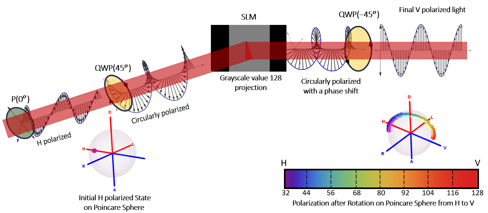
IX Realization of Polarization Grating through a Spatial Light Modulator
In this section, we describe the realization of the polarization grating using polarization optics and a spatial light modulator (SLM) [30]. As shown in Fig. 5, the polarization rotation of the input beam is performed using a SLM in combination with two quarter-wave plates (QWPs). Specifically, the input beam is prepared by passing it through a polarizer aligned to the H polarization. The beam first passes through a QWP at an angle of . Then, this beam is imprinted on the SLM, where a gray-value image is displayed. Finally, the reflected beam passes through another QWP at an angle of . This configuration provides the ability to rotate the polarization of the incident beam in a controlled fashion. We then characterize the relationship between the polarization rotation and the gray-value displayed on the SLM. This allows us to design a gray-scale image to implement the polarization grating. By adjusting the gray-scale values across different pixels along the -axis of the SLM screen, we can control the polarization at each pixel. We can thus simulate the effect of a polarization grating on an unpolarized light source.