Emergent behaviors of rotation matrix flocks
Abstract.
We derive an explicit form for the Cucker-Smale (CS) model on the special orthogonal group by identifying closed form expressions for geometric quantities such as covariant derivative and parallel transport in exponential coordinates. We study the emergent dynamics of the model by using a Lyapunov functional approach and La Salle’s invariance principle. Specifically, we show that velocity alignment emerges from some admissible class of initial data, under suitable assumptions on the communication weight function. We characterize the -limit set of the dynamical system and identify a dichotomy in the asymptotic behavior of solutions. Several numerical examples are provided to support the analytical results.
Key words and phrases:
Cucker-Smale model, special orthogonal group, emergence, flocking, velocity alignment, rotation group.2020 Mathematics Subject Classification:
70G60, 82C10
1. Introduction
Collective behaviors of complex biological systems are ubiquitous in nature, e.g., aggregation of bacteria [36, 58], synchronous flashing of fireflies [9], synchronization of rhythms in pacemaker cells [47], flocking of migratory birds [7, 52] and swarming of fish [5, 16, 57]. We refer to [4, 46, 48, 62] for a brief survey of collective dynamics and engineering applications in the decentralized control of multi-agent systems. Among them, our main interest lies in flocking behaviors in which particles organize themselves from a disordered state to an ordered motion using simple rules based on environmental information. Despite its ubiquitous presence, systematic mathematical studies have begun only several decades ago by Vicsek et al. [61], a group of statistical physicists who were mainly motivated by Reynolds’s simulations [52] of bird flocking in computer graphics. Since then, several mechanical and phenomenological models have been used to study flocking behavior.
In this paper, we are interested in the Cucker-Smale (CS) model [13] for flocking of a matrix ensemble on the special orthogonal matrix group , given by:
| (1.1) |
where is the matrix group consisting of all real matrices and denotes the identity matrix. Note that , also referred to as the rotation group, is a Lie group, having a group and a manifold structure at the same time. Elements in are called rotation matrices; they are characterized by an axis and an angle of rotation. The rotation group is the configuration space of a rigid body in that undergoes rotations only (no translations). There has been recent growing interest in studying collective behavior on [15, 14, 31], motivated by body attitude coordination of interacting agents in a variety of applications. For example, engineering applications include synchronization of satellite attitudes [8, 37, 39] and camera pose averaging [60]. In biology, it is very common for animals such as birds and fish to coordinate their body attitudes – see [15] for some images of collective motions in birds and dolphins.
Before we present the CS model on , we introduce the CS model on the Euclidean space . Consider an ensemble of identical particles with unit mass in , and let and be the position and velocity of the -th particle, respectively. The CS model reads:
| (1.2) |
where is a nonnegative coupling strength and are communication weights given in terms of a bounded and Lipschitz continuous communication function . In this setting, the global well-posedness of (1.2) follows directly from the Cauchy-Lipschitz theory together with uniform boundedness of the kinetic energy. The CS model (1.2) exhibits interesting flocking dynamics depending on the initial configuration, system parameters and communication functions (see [13, 32, 34]), and it has been studied extensively in applied mathematics and control communities in the last decade. The model has been investigated in diverse directions and areas of applications, e.g., network topology [11, 12, 20, 21, 41, 42], global and local flocking dynamics [13, 32, 34, 45], interaction with nonlinear damping [22], time-delayed interactions [17], kinetic and hydrodynamic CS equations [18, 40, 50, 51, 55, 56], coupling with thermodynamics [26, 27, 30, 33], complete predictability [28], extension to manifolds [1, 2, 3, 31] and relativistic CS model [29]. We refer to recent survey articles [4, 10, 44] for overview and further references.
In the present paper we address the“Cucker-Smale flocking realizability problem” on :
-
•
(Q1): Is there a CS type flocking model on ?
-
•
(Q2): If so, under what conditions on system parameters and initial data, can we guarantee emergent dynamics?
To answer question (Q1), we need to replace the R.H.S. of by a suitable internal force so that particles’ positions stay on through the time evolution. This is not obvious at first glance, as we need to compare velocities belonging to different tangent spaces. In fact, question (Q1) was already answered affirmatively in an abstract setting in which the underlying manifold is a connected, complete and smooth Riemannian manifold with a metric (see [31]), whereas question (Q2) was answered only for the sphere and the hyperboloid (see [2, 3]).
Specifically, let ( be a connected, complete and smooth Riemannian manifold with metric . Denote by the covariant derivative of a tangent vector . For , let be the parallel transport along the length minimizing geodesic from to . In this abstract Riemannian setting, the CS model on takes the following form:
| (1.3) |
where is a nonnegative coupling strength and are communication weights. Here, denotes the geodesic distance on , and the communication weight function is assumed to be a nonnegative, bounded, and smooth function on . Note that the parallel transport in model (1.3) is well-defined only if the length minimizing geodesic between and is unique, i.e., when the two points are not in the cut locus of each other. To alleviate this issue, if two points are in the cut locus of each other then we set to be zero for such pairs of points111In the paper we will use the term pair of cut points to refer to two points on a manifold that are in the cut locus of each other., so that system (1.3) is well-defined and the local well-posedness of (1.3) is guaranteed. For certain special manifolds, one can explicitly calculate and , and write the abstract CS model (1.3) in an explicit form. Examples of such manifolds are the Poincaré Half plane [31], unit sphere [2, 31] and hyperboloid [3]. For related first-order aggregation models on Riemannian manifolds, we also refer to [6, 23, 24, 25, 43, 53, 54].
We adopt the following definition of velocity alignment.
Definition 1.1.
Next, we discuss briefly our main results. To simulate the particle system on a specific manifold, the abstract model (1.3) cannot be used directly, unless we find an explicit form for equation . Our first main result is concerned with the explicit derivation of the CS model on by finding closed-form representations for and . For the model on we will use and instead of and , to denote the position and velocity of the -th particle at . Since lies in the tangent space of at , there exists a unique skew-symmetric matrix (see Section 2) such that
To close the dynamical system we need to find the dynamics for or from . In order to present this explicit form, we need some preparations. First note that , the Lie algebra of consisting of all skew-symmetric matrices, is isomorphic to via the hat map:
| (1.4) |
For given , we set
where denotes the Euclidean norm in . The precise meanings of these variables will be given in Section 2. Equipped with these notations, the CS model on is given by:
| (1.5) |
where satisfies .
As noted above, parallel transport between a pair of cut locus points is not well-defined, and in such cases we require that the communication weighs between the points is zero. On , the injectivity radius is and two rotation matrices and are in the cut locus of each other if and only if . For system (1.5) to be well-defined and also locally well-posed, one of the following conditions will be used later.
-
•
: is a continuous function of that vanishes at pairs of cut locus points:
-
•
: for any and , the distance between and is strictly less than .
Our second main results deal with the emergent dynamics of (1.5). For this, we introduce a Lyapunov functional given by the total kinetic energy:
Then, by straightforward calculations, one can derive a dissipation estimate (see Section 4.3) :
| (1.6) |
We apply LaSalle’s invariance principle [38] and use (1.6) to obtain
Under the assumptions or , one can then derive velocity alignment (Theorem 4.1).
Finally, we characterize the -limit set of model (1.5), and show that a certain dichotomy holds in the asymptotic behavior of the solutions (Theorem 4.2). This result is confirmed by numerical simulations.
The paper is organized as follows. In Section 2, we review briefly the geometry of the rotation group, e.g., the exponential map, the explicit form of the metric tensor, geodesic equations, as needed for later sections. In Section 3, we provide equations for geodesics and provide a closed form representation for parallel transport and its geometric interpretation. In Section 4, we explicitly derive the CS model on from the abstract model (1.3) and study its emergent dynamics. In Section 5, we provide several numerical simulations and compare them with the analytical results in previous sections. Finally Section 6 is devoted to a brief summary of our main results and some remaining issues for future work. In Appendix we provide proofs for several lemmas and details to various calculations used in the paper.
Gallery of Notation: For notational simplicity, we use the following handy notation:
and if there is no confusion, we also use Einstein’s notation on repeated indices from time to time. Let be the collection of real matrices and for , we introduce the Frobenius inner product and its associated norm:
2. Geometry of the special orthogonal group
In this section, we review minimal background on the geometry of the special orthogonal group which will be necessary to follow discussions in later sections. In particular, we present as a Riemannian manifold and derive explicit calculations using the parametrization by exponential coordinates.
2.1. General considerations
The Lie algebra of the Lie group in (1.1), representing the tangent space of at the identity , is given by:
where is the zero matrix. In general, the tangent space at a generic point is given by
| (2.1) |
The Riemannian metric on is defined as:
| (2.2) |
for any . Note that the norm induced by the metric satisfies
| (2.3) |
Throughout the paper, we use for the usual vector norm in , for the Frobenius norm, and for the Riemannian norm at . We also denote the Frobenius and the Riemannian inner products by and , respectively. In summary, we have the following relations between the Frobenius and Riemannian norms/inner-products as follows:
where , , and are tangent vectors in .
2.1.1. Isomorphism between and
To any vector we associate its corresponding skew-symmetric matrix given by (1.4). By introducing the canonical basis of :
| (2.4) |
the hat operation can be expressed as:
| (2.5) |
where we used the Einstein convention for summation over repeated indices. Note that the components of , can be also expressed as
where denotes the Levi-Civita symbol.
The inverse of the hat map, denoted by , is given by:
The hat operator (and its inverse) establish an isomorphism between and . In particular, , for all .
2.1.2. Angle-axis representation
As mentioned in the Introduction, an element in is called a rotation matrix. Hence, any rotation can be identified with a pair , where denotes the unit sphere in . The unit vector indicates the axis of rotation and represents the angle of rotation (by the right-hand rule) about the axis . The pair is also referred to as the angle-axis representation of the rotation . The expression of in terms of is given by the exponential map via Rodrigues’s formula:
| (2.6) |
The inverse of Rodrigues’s formula, , is also given by
| (2.7) |
2.1.3. Geodesic distance, exponential and logarithm maps
Given two rotation matrices , , the shortest path between and is the geodesic curve given by
Note that
and the Riemannian distance between and on on is
where satisfies
Then by (2.7), we also have
| (2.8) |
and in particular, .
2.2. Exponential coordinates
For fixed , we introduce exponential coordinates (also commonly referred to as Riemannian normal coordinates [49]) on centerd at . With this aim we consider the map (see (2.9)) given by
| (2.10) |
which is an injective map on . The chart covers all but the cut locus of . Throughout the paper, we will use Greek letters (, etc) for coordinates on . Consequently, indices in Greek letters take values in . We make this distinction to avoid possible confusion with indices for particles in the Cucker-Smale model, for which we use Roman letters (, etc); such indices take values in . First, we compute the basis of the tangent space at induced by the coordinate chart (2.10). By differentiating (2.10), we have
| (2.11) |
We set
| (2.12) |
Then, we use (2.6) to find
This yields,
| (2.13) |
Lemma 2.1.
For any , one has
| (2.14) |
where denotes the anticommutator .
Proof.
Remark 2.1.
In the following lemma, we list several other elementary results to be used later.
Lemma 2.2.
For , let be given by (2.5) and . Then the following identities hold:
Proof.
See Appendix A.1. ∎
2.3. The metric tensor
In this subsection, we derive explicit representations for the metric tensor and its inverse . First, we study a set of elementary estimates in the following lemma.
Lemma 2.3.
For , let be given by (2.5) and . Then, the following identities hold
Proof.
(i) By direct calculation, one can find
Then, one has
and
(ii) Since the derivations for identities in (ii) are rather lengthy, we present them in Appendix A.2. ∎
Proposition 2.1.
For , let be given by (2.5) and . Then, the metric tensor and its inverse are given as follows.
Proof.
(i) It follows from (2.2) and
that
| (2.16) |
On the other hand, since and are skew-symmetric, is also symmetric. Now, we decompose (2.15) in skew-symmetric and symmetric parts:
| (2.17) |
where and are skew-symmetric and symmetric matrices, respectively. One finds:
Next, we combine (2.16) and (2.17) to find
| (2.18) |
where we used that for any skew-symmetric matrix and symmetric matrix . For the estimation of the two terms in the R.H.S. of (2.18), we use Lemma 2.3.
Estimate of : We use Lemma 2.3 (i) to find:
| (2.19) |
2.4. Christoffel symbols and geodesic equations.
A direct calculation in Appendix A.4 and formula for the Christoffel symbols
yield
| (2.22) |
One advantage of working with exponential coordinates is that geodesics are images of straight lines under the parametrization map. To check the expressions (2.22), it can be shown that for a fixed vector , the straight line satisfies the geodesic equations
for all . The second derivative is zero, so we only need to check
| (2.23) |
Detailed arguments will be given in Appendix A.5.
3. Parallel transport on
In this section we derive an explicit formula for the parallel transport on along a geodesic, and provide its geometric interpretation.
3.1. Parallel transport
Consider a geodesic curve on given in exponential coordinates by , for a fixed , and the parallel transport along this geodesic of a vector of components . Then, the equations for parallel transport are given by
Since along the geodesic, we can write the equations as
| (3.1) |
Next, we calculate with the Christoffel symbols given by (2.22). By direct substitution of in (2.22) (in particular, use ), we obtain
| (3.2) |
where the second equal sign follows from elementary algebra and .
For calculations in this section we reset the notation for used in Section 3, and denote:
With this notation, rewrite (LABEL:AC-1) as
Then, we use the above expression in the equations (3.1) for parallel transport to find
| (3.3) |
Multiply both sides of (3.3) by and sum up the resulting relation over to obtain
The second term in the R.H.S. above vanishes, and the vector is constant. This leads to
and hence is a conserved quantity:
| (3.4) |
for a constant . The conservation property in (3.3) implies
| (3.5) |
To find the exact solution of (3.5), we define the function by
| (3.6) |
Here we can easily check that is a function defined on , and satisfies
so one can write (3.5) as
Furthermore, we have
This implies
which yields the explicit solution of the parallel transport equations (3.1):
| (3.7) |
with and given by (3.4).
3.2. Coordinate-free closed form expression
We use the explicit formula (3.7) to derive a coordinate free expression for parallel transport along a geodesic. We fix , with , and consider the unique geodesic path between them. We set exponential coordinates centered at , and also set by
Equivalently one has
The geodesic curve between the two matrices is given by
In particular, represents the geodesic distance between and (see (2.8)):
Also, by (2.7), the unit vector satisfies:
For notational convenience, we adopt the following notation for the tangent vectors in exponential coordinates (see (2.11) and (2.15)):
Then, it follows from (2.11) and (2.15) that
| (3.8) |
Now take a tangent vector given in components by
| (3.9) |
According to the calculations performed in Section 3.1 (see equation (3.7)), the parallel transport of from to along the geodesic curve is
| (3.10) |
where
Here, is the constant of motion given by (3.4). Using (3.6) and some simple manipulations we write the components of as
| (3.11) |
3.3. A geometric interpretation
By (2.1), the tangent vectors and take the following form:
where and are skew-symmetric matrices. To provide better insight, which leads to a nice geometric interpretation of parallel transport, we now express (3.12) in terms of these skew-symmetric matrices.
Therefore, we set
| (3.13) |
and also define and such that and For convenience of notation, denote
Then, it follows from (3.12) that
| (3.14) |
We take the transpose in Rodrigues’s formula (2.6) (applied to ) to get
| (3.15) |
Hence, one has
| (3.16) |
where we used that (see Lemma 2.1).
By using (3.15) and (3.16) in (3.14), after some manipulations (see Appendix A.7), we derive the following expression for :
| (3.17) |
The expression for can be further simplified using the following lemma.
Lemma 3.1.
Let and their corresponding skew-symmetric matrices . The following identities hold:
| (3.18) |
Proof.
See Appendix A.8. ∎
First note that by , (3.9) and (3.13), we have:
and hence, by (3.4),
Then, it follows from and that
Using the equations above, combine the first and third terms in the R.H.S. of (3.17) to get
| (3.19) |
where we also used
Remark 3.1.
Remarkably, (3.21) is in the form of Rodrigues’ rotation formula, with representing the rotation (according to the right-hand-rule) of about the axis by an angle . For the case in which is in the direction of , we have as expected.
Parallel transport by general theory on Lie groups. In [35, Chapter 2], listed as an exercise, one can find a general expression for parallel transport along geodesics on connected Lie groups. Specifically, consider a connected Lie group with Lie algebra , endowed with an affine connection that is invariant under left and right translations and under the map . For , denote by and the left and right translations by , respectively. Take . The parallel translate of along the geodesic , , is given by:
The rotation group and its connection satisfy the assumptions to apply the formula for parallel transport above. Adapting it to the setup of , we can find that the parallel transport of from to is given by:
This is equivalent to
or using Rodrigues’ formula:
| (3.22) |
where .
Next, we expand the R.H.S. of (3.22) and show that it is the same as that of (3.19). Indeed, we have
| (3.23) |
where the terms containing and have been cancelled out; this cancellation comes from the fact that , since by .
By direct calculation, one can show
Using these identities in (3.23), (3.22) becomes:
Finally, combine the terms containing to get (3.19).
While our expression for parallel transport is consistent with this general result on Lie groups, it presents an elementary and hands-on approach to its derivation. We are not aware of any other works presenting the explicit forms of the metric tensor, Christoffel symbols, geodesics and parallel transport in exponential coordinates, as done in Sections 2 and 3. These explicit calculations would be valuable tools for researchers on rigid-body dynamics.
4. The CS model on
In this section, we provide a derivation of the CS model on by gathering calculations from previous sections, and investigate its emergent dynamics. We also study the reduction of the model to .
4.1. Formulation of the CS model on
Let be the position of the -th CS particle, and we set its velocity as
| (4.1) |
Note that we require to satisfy (see (1.3)):
| (4.2) |
Since lies in the tangent space of at , there exists a unique skew-symmetric matrix such that
This yields
| (4.3) |
We will rewrite (4.2) in terms of . By definition of the covariant derivative (using the embedding of in ), one has:
| (4.4) |
Then, it follows from (4.3) and (4.4) that
where we used the fact that is symmetric and is skew-symmetric. This and (4.2) yield
| (4.5) |
We use now the calculations in Section 3.2. Here, and play the roles of and from these calculations, while and play the roles of and . In particular, plays the role of , and plays the role of . Also, analogous to , and from Section 3.2, we have and , defined by:
| (4.6) |
From this framework, apply the parallel transport formula (3.20) to get
| (4.7) |
where we denoted
| (4.8) |
Then, using (4.7) in (4.5) yields
or equivalently, by removing the hats,
| (4.9) |
Since parallel transport between two cut locus points cannot be well defined, we should impose some conditions on or a priori conditions (see and ). Some examples of communication weight functions that satisfy condition are:
The well-posedness of the CS model on is given by the following proposition.
Proposition 4.1.
Suppose either or holds. Then, the Cauchy problem to system (4.10) has a unique global solution.
Proof.
Case A: Suppose the first condition holds. Then and are Lipschitz continuous functions in the whole domain. Therefore, standard Cauchy-Lipschitz theory and continuity argument based on uniform a priori bound yield the global well-posedness of a smooth solution.
Case B: Suppose the second condition holds. Then and are Lipschitz continuous functions in the whole domain, except at cut locus pairs. Then, similar to Case A, one can guarantee the global unique solvability of the Cauchy problem to (4.10). ∎
4.2. Reduction from to
In this subsection, we study the relation between the CS model on and the CS model on the circle .
Suppose that the initial data are given as follows.
Then, by the isomorphism between and in Section 2.1.1, one has
Now take the following ansatz for the solution and :
| (4.11) |
where
Then we have
From here, one has
By direct calculation, we have
So we set
to satisfy . Since and are parallel, and is a unit vector, it holds that
From these relations, we have
Hence, if satisfy the CS model on the circle, given by:
then defined by (4.11) satisfy (4.10). This shows that in this case, the CS model on can be reduced to the CS model on the circle.
4.3. Emergent dynamics
In this subsection, we study the emergent behavior of the CS model (4.10) by using an explicit Lyapunov functional and LaSalle’s invariance principle. For a given ensemble , we define a Lyapunov functional which corresponds to the total kinetic energy:
Then, by direct calculations, one has
| (4.12) |
For the last two equalities in (4.12), we used the symmetry of the communication function, , and the fact that parallel transport preserves lengths, specifically,
Let be a solution of system (4.10). From (4.12), we know that is decreasing, and hence,
which implies the boundedness of for all and . Then, by defining the subset of ,
we can restrict the domain of states as follows:
Since this domain is compact, we can apply LaSalle’s invariance principle to (4.12) to get
| (4.13) |
On the other hand, using (3.20) and the fact that the hat operator is an isomorphism between and , one has:
| (4.14) |
Theorem 4.1.
Suppose that either or in Section 1 holds, and let be a solution to (4.10). Then, one has the following assertions.
-
(1)
Suppose that the condition holds. Then, for each we have
(4.15) or equivalently,
-
(2)
Suppose that the condition holds. Then, for each we have
or equivalently,
4.4. The -limit set
In this subsection, we investigate the structure of the -limit set of the Cucker-Smale model on . By Theorem 4.1, each point in the -limit set satisfies (4.15). Moreover, since the -limit set is positively invariant, each trajectory that starts in the -limit set satisfies . Therefore, each particle is either at rest or moves along a constant speed geodesic.
Geodesic loops in . Let us first specify what is a closed geodesic curve on . Consider the unit-speed geodesic curve starting at in the direction , where , with . By the explicit representation of the exponential map in (2.9), this curve is given as
At , is a point in the cut locus of , at distance from .
Now consider the unit-speed geodesic curve starting from in the opposite direction , as given by
This curve reaches the same point at time . By construction,
In particular, the tangents to the two curves at are opposite to each other, that is,
To obtain a geodesic loop starting and ending at we patch together the two geodesic arcs, and consider the curve on defined by:
Then, we can extend the curve for all , with the image of the curve being this closed geodesic loop.
In the visualization of as a ball of radius with center at (see also Section 5), this geodesic loop consists of two parts. The first part is the curve starting at the center and reaching the boundary (the sphere of radius ) at . The second part of the loop starts at the antipodal of the point where the first curve ended at , and ends at the center . So visually, it seems like that a jump has occurred at , however, antipodal points on the boundary are identified, and the curve is indeed smooth.
Structure of the -limit set. Consider constant speed geodesic loops on , as described above, initialized in the -limit set of (4.10). The loops start at , in the direction , where , , are constant matrices. Note that have not been assumed of unit length, so a generic loop closes after units of time. For all , we have
For the moment, we ignore the issue of points reaching the cut locus of each other dynamically. To characterize the -limit set of the CS model (4.10), we require
| (4.16) |
such that . The goal is to show that the only possibility for this to happen is to have a single geodesic loop along which all particles move.
Fix two arbitrary indices and and suppose that . Then there exists such that
Consider , the length-minimizing geodesic between and , and the parallel transport of along , from to . Using the calculations detailed in Section 4.1 (see equation (4.7)), the parallel transport relationship (4.16) can be written as:
| (4.17) |
or without the hats,
| (4.18) |
where we used notations (4.6) and (4.8). Note that and depend on time, while and are fixed. Equations (4.17) (and (4.18)) need to hold for all times.
First, since parallel transport preserves lengths, we have
or equivalently, . We denote by the common length, and hence we can write
| (4.19) |
where and are unit vectors in .
Second, parallel transport preserves angles, so the angle that makes with the geodesic at is the same as the angle between and at . Consequently,
and hence, we have
| (4.20) |
By the expression of matrix logarithm (see (2.7)), we can write (4.20) as
and furthermore, by restoring the dependence on ,
The expression is well-defined when . Since the function can be extended to continuously, we define the value at as .
Now we work out the following equation explicitly:
| (4.21) |
Note that for any skew-symmetric matrix and rotation matrix , one has
Hence, since is skew-symmetric and , (4.21) can be written as
or equivalently,
| (4.22) |
Since and (see (4.19)), we can cancel and write (4.22) as:
| (4.23) |
In the following lemma, we calculate and .
Lemma 4.1.
The following relations hold:
where we used the notation .
Proof.
Since the proof of this lemma is rather lengthy, we present it in Appendix A.9. ∎
We substitute the result of Lemma 4.1 into (4.23) and equate the coefficients of the trigonometric functions , , , and to obtain
| (4.24) |
From , we get
| (4.25) |
Then, (4.25) and yield
| (4.26) |
Note that can be rewritten as
| (4.27) |
Finally, leads to
| (4.28) |
Without any loss of generality, we assume that is a rotation about the -axis. Since , the angle of rotation is . For simplicity of notation, set
Then becomes
Also for ease of notation, we set
By direct calculation, one finds
For , (4.26) implies
By direct calculations one finds
Note that since depends only on , one has
Hence, we can combine (4.27) and (4.28) to get
and by using the coordinate expressions for the two traces, we find
| (4.29) |
By using one finds that equation (4.25) leads to an identity, with both sides being equal to
Finally, (4.27) yields
| (4.30) | ||||
We solve equations (4.29) and (4.30) for unknowns and . By direct (but tedious) calculations, the two sets of solutions turn out to be:
or in vector form,
Note that the latter solution satisfies
Next we study the two cases separately.
Case A (; also, , and ): Recall from the geometric interpretation of (4.18) that at all times, can be obtained as the rotation by right-hand-rule of about the axis , by an angle . In particular, this statement holds at . Provided , a rotation keeps a vector unchanged only if the vector is parallel to the rotation axis. Hence, , which implies that the particles move along the same geodesic loop, which includes the geodesic curve between and . In the trivial case , one gets and for all . Note that moving along the same geodesic loop, the distance between the two particles remains constant in time, that is, for all .
Case B (, or equivalently ): Note that is a rotation about by angle . This can only be consistent with the geometric interpretation of (4.18) provided or equivalently , in which case we get for all .
The considerations above lead to the following proposition.
Proposition 4.2.
Proof.
Fix an index and take another generic index . If , the discussion above applies and we have
where and . Furthermore, and rotate on the same closed geodesic curve. Note that when this reduces to the trivial case and , for all .
Consider now the case . The matrices and are governed by the dynamics
for constant matrices . If , then for , where is a sufficiently small positive constant. Then we can restart the time and apply the result for the first case, to obtain that , which gives a contradiction. Therefore, we have in this case as well.
When particles satisfy for all , the first case applies to the entire group and all particles rotate along the same closed geodesic curve. ∎
The main result of this section is the following dichotomy on the long time behavior of the CS model on SO(3).
Theorem 4.2.
Let be a solution of (4.10). Then, we have the following dichotomy for its asymptotic dynamics:
-
(1)
either the kinetic energy tends to zero:
-
(2)
or the kinetic energy converges to a nonzero positive value , and
(4.31) (4.32)
Proof.
It follows from (4.12) that is non-increasing. Since , there exists a limit:
| (4.33) |
If , we can obtain the first case. Now we assume that .
By LaSalle’s invariance principle we infer that
| (4.34) |
where and is the -limit set of system (4.10). From Proposition 4.2, we know that any state in satisfies
If we combine this fact with (4.34), we can then obtain (4.31).
Note that the asymptotic behavior in (4.31) only states that the differences between and converge to zero for all . In particular, (4.31) does not imply that each converges to some fixed as . On the other hand, one can show that the norms have a common fixed limit as . To show this, express the energy functional as:
By (4.33) we then have
| (4.35) |
For a fixed index , we have
Letting in the equation above and using (4.35), we get
| (4.36) |
Now combine (4.31) and (4.36) to obtain
which yields (4.32).
∎
Remark 4.1.
As noted above, (4.31) does not imply that each converges to a fixed skew-symmetric matrix as . Consequently, the directions of motion of the particles are not guaranteed to have a limit as . By (4.32) however, the particles’ speeds become equal asymptotically. Numerical simulations suggest (see Section 5) that the directions of motion of the particles have in fact a common limit as , meaning that asymptotically, particles approach and rotate with constant speed along a common geodesic.
5. Numerical Simulations
We solve numerically the CS model on using the 4th order Runge-Kutta method. In the simulations presented below we initialize the rotation matrices in the angle-axis representation (see Section 2.1.2). Specifically, the rotation angles () were initialized randomly in the interval , while the unit vectors were generated in spherical coordinates, with the polar and azimuthal angles drawn randomly in the intervals and , respectively. For the initial velocities (), we generate the components of (here, ) randomly in the interval .
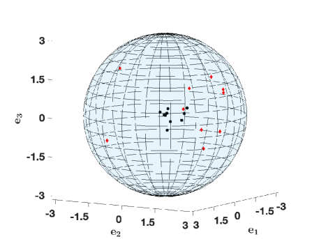
For plotting purposes, is identified with the ball in of radius , centered at the origin. The center of the ball corresponds to the identity matrix . A generic point within the ball represents a rotation matrix, with rotation angle given by the distance from the point to the center, and axis given by the ray from the center to the point. Antipodal points on the surface of the ball are identified, as they represent the same rotation matrix (rotation by about a ray gives the same result as rotation by about the opposite ray).
The numerical results we present correspond to the communication function
Note that this function vanishes for pairs of cut points, i.e., for . Similar results were obtained with other communication functions as well.
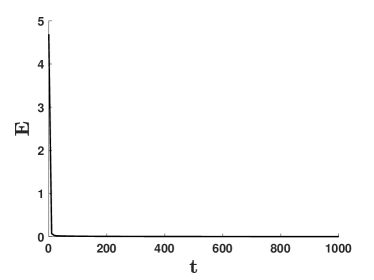
Figure 1 corresponds to a simulation where all particles come to a stop asymptotically. In Figure 1(a) the initial and final locations of the particles are indicated by black dots and red diamonds, respectively. At particles have reached a configuration with an energy of order . Also note the decay to over time of the energy, as shown in Figure 1(b).
 |
 |
| (a) | (b) |
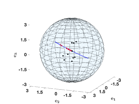
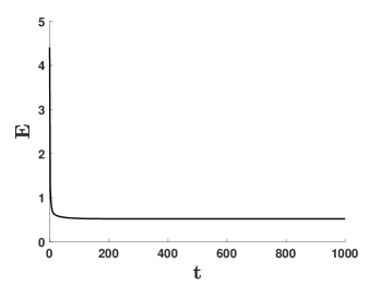
Figure 2 shows a simulation in which particles reach asymptotically a flocking state. In Figure 2(a) the initial locations of the particles are indicated by black dots. At the particles (red diamonds) have aligned along the closed geodesic path indicated by small blue dots, and we will rotate on this closed geodesic loop indefinitely. Note that the initial and end points of the geodesic path are antipodal of each other and hence, by the visualization of that we use, they represent the same rotation matrix. Therefore, the geodesic path is in fact closed, though it does not appear so in the figure. Figure 2(b) shows the energy decay over time. As opposed to the previous simulation, the energy now approaches a non-zero value as , as particles do not stop, but keep moving on the geodesic loop.
 |
 |
| (a) | (b) |
6. Conclusion
In this paper, we have studied the Cucker-Smale model on which exhibits collective behaviors of a rotation matrix ensemble. In earlier work [31], a general and abstract Cucker-Smale model was proposed on a connected, complete and smooth Riemannian manifold using the covariant derivative and parallel transport of tangent vectors along length minimizing geodesics. Thus, for the explicit dynamics and numerical simulations of particles lying on a given specific Riemannian manifold, one needs to find explicit forms for the covariant derivative and parallel transport in terms of state variables and the underlying geometric information. Fortunately, for the special orthogonal group, we can explicitly calculate the covariant derivative and parallel transport which results in the explicit representation of the Cucker-Smale model on . For the proposed model, we used a Lyapunov approach based on an energy functional. By deriving a dissipative estimate, we use La Salle’s invariance principle to conclude the velocity alignment without any a priori conditions.
Of course, there are still various issues that have not been addressed in the current work, for example, we do not have explicit information on the spatial structure of emerging asymptotic configurations and asymptotic velocity, due to the lack of enough conservation laws, etc. These interesting issues will be addressed in future work.
Appendix A Proofs of several lemmas
In this appendix, we present proofs of several lemmas and details to various calculations employed in the main body of the paper.
A.1. Proof of Lemma 2.2.
By direct calculation, one has
| (A.1) |
This yields
which shows the first identity.
We verify the second identity for . The other cases can be treated similarly.
Furthermore,
Similarly one check the identity for and .
A.2. Proof of Lemma 2.3.
We provide derivations for the following three identities:
(Derivation of the first identity): we use (A.1) to calculate
(Derivation of the second identity): we use the commutativity of the trace to get
| (A.2) |
Then use the first identity in Lemma 2.1 and the fact that is skew-symmetric to find
| (A.3) |
Finally, we combine (A.2), (A.3) and the third identity in Lemma 2.2 to obtain the desired second identity.
(Derivation of the third identity): Note that
| (A.4) |
Next, we want to express
for general . To simplify this term, we will use the notation introduced in Remark 2.1. We use Einstein’s convention (repeated index means summation) to find
| (A.5) |
where we used in last equality. Now we combine (LABEL:Ap-3) and (A.5) to get
A.3. Inverse of the metric tensor
A.4. Christoffel symbols (2.22)
A.5. Equation (2.23) for geodesics
A.6. Closed form expression (3.12) of parallel transport
A.7. Expression (3.17) for
We use (3.15), (3.16) in (3.14) and arrange terms to get
| (A.11) |
After some simple trigonometric manipulations, we can write (A.11) as
| (A.12) |
To derive further simplification of (A.12), we present an elementary lemma as follows.
Lemma A.1.
Proof.
A.8. Proof of Lemma 3.1
Take , in .
Then, from (A.13) we have
Since the matrix on the r.h.s. above is , we get the second identity in (3.18).
Finally, also from (A.13), we get
A.9. Proof of Lemma 4.1.
(i) By the explicit formula of and , we have
Recall that and (see (4.19)). Hence, we have:
| (A.14) |
where we used Rodrigues’s formula and the notation .
Note that
| (A.15) |
where we used that for the second equal sign. Now, by the trigonometric identities:
we write the R.H.S. of (LABEL:New-3) as a linear combination of trigonometric functions:
| (A.16) |
Combining (LABEL:eqn:term1), (LABEL:New-3) and (LABEL:eqn:calc1) leads to identity (i) in Lemma 4.1.
(ii) Similarly, one has
| (A.17) |
Note that
| (A.18) |
By writing the R.H.S. as a linear combination of trigonometric functions we find:
| (A.19) |
Combining (LABEL:eqn:term2), (LABEL:New-4) and (LABEL:eqn:calc2) leads to identity (ii). ∎
References
- [1] Ahn, H., Ha, S.-Y. and Shim, W.: Emergence dynamics of the discrete-time thermodynamic Cucker-smale model on Riemannian manifolds. Submitted.
- [2] Ahn, H., Ha, S.-Y. and Shim, W.: Emergent dynamics of a thermodynamic Cucker-Smale ensemble on complete Riemannian manifolds. To appear in Kinetic and Related Models.
- [3] Ahn, H., Ha, S.-Y., Park, H., and Shim, W.: Emergent behaviors of Cucker-Smale flocks on the hyperboloid. Submitted.
- [4] Albi, G., Bellomo, N., Fermo, L., Ha, S.-Y., Pareschi, L., Poyato, D. and Soler, J.: Vehicular traffic, crowds, and swarms. On the kinetic theory approach towards research perspectives. Math. Models Methods Appl. Sci. 29 (2019), 1901-2005.
- [5] Aoki, I.: A simulation study on the schooling mechanism in fish. Bulletin of the Japan Society of Scientific Fisheries. 48 (1982), 1081-1088.
- [6] Aydodu, A., McQuade, S. T. and Pouradier Duteil, N.: Opinion dynamics on a general compact Riemannian manifold. Netw. Heterog. Media 12 (2017), 489-523.
- [7] Ballerini, M., Cabibbo, N., Candelier, R., Cavagna, A., Cisbani, E., Giardina, I., Lecomte, V., Orlandi, A., Parisi, G., Procaccini, A., Viale M. and Zdravkovic, V.: Interaction ruling animal collective behavior depends on topological rather than metric distance: Evidence from a field study. Proc. Natl. Acad. Sci. USA 105 (2008), 1232-1237.
- [8] Bondhus, A. K., Pettersen, K. Y. and Gravdahl, J. T.: Leader/follower synchronization of satellite attitude without angular velocity measurements. Proc. 44th IEEE Conf. on Decision and Control, pages 7270–7277, 2005.
- [9] Buck, J. and Buck, E.: Biology of synchronous flashing of fireflies. Nature 211 (1966), 562-564.
- [10] Choi, Y.-P., Ha, S.-Y. and Li, Z.: Emergent dynamics of the Cucker-Smale flocking model and its variants. In N. Bellomo, P. Degond, and E. Tadmor (Eds.), Active Particles Vol.I Theory, Models, Applications, Series: Modeling and Simulation in Science and Technology, Birkhauser, Springer. 2017.
- [11] Cucker, F. and Dong, J.-G.: On flocks influenced by closest neighbors. Math. Models Methods Appl. Sci. 26 (2016), 2685-2708.
- [12] Cucker, F. and Dong, J.-G.: On flocks under switching directed interaction topologies. SIAM J. Appl. Math 79 (2019), 95-110.
- [13] Cucker, F. and Smale, S.: Emergent behavior in flocks. IEEE Trans. Automat. Contr. 52 (2007), 852-862.
- [14] Degond, P., Diez, A., Frouvelle, A. and Merino-Aceituno, S.: Phase Transitions and Macroscopic Limits in a BGK Model of Body-Attitude Coordination. J. Nonlinear Sci. 30 (2020), 2671–2736.
- [15] Degond, P., Frouvelle, A. and Merino-Aceituno, S.: A new flocking model through body attitude coordination. Math. Models Methods Appl. Sci. 27 (2017), 1005-1049.
- [16] Degond, P. and Motsch, S.: Large-scale dynamics of the Persistent Turing Walker model of fish behavior. J. Stat. Phys. 131 (2008), 989-1021.
- [17] Erban, R., Haskovec, J. and Sun, Y.: On Cucker-Smale model with noise and delay. SIAM J. Appl. Math. 76 (2016), 1535-1557.
- [18] Fornasier, M., Haskovec, J. and Toscani, G.: Fluid dynamic description of flocking via Povzner-Boltzmann equation. Physica D 240 (2011), 21-31.
- [19] do Carmo, M. P.: Riemannian geometry. Mathematics: Theory and Applications, Birkhäuser.
- [20] Dong, J.-G., Ha, S.-Y., Jung, J. and Kim, D.: On the stochastic flocking of the Cucker-Smale flock with randomly switching topologies. SIAM J. Control Optim. 58 (2020), 2332-2353.
- [21] Dong, J.-G. and Qiu, L.: Flocking of the Cucker-Smale model on general digraphs. IEEE Trans. Automat. Control 62 (2017), 5234-5239.
- [22] Fang, D., Ha, S.-Y. and Jin, S.: Emergent behaviors of the Cucker-Smale ensemble under attractive-repulsive couplings and Rayleigh frictions. Math. Models Methods Appl. Sci. 29 (2019), 1349-1385.
- [23] Fetecau, R., Ha, S.-Y. and Park, H.: An intrinsic aggregation model on the special orthogonal group : well-posedness and collective behaviors. Submitted.
- [24] Fetecau, R., Park, H. and Patacchini, F. S.: Well-posedness and asymptotic behavior of an aggregation model with intrinsic interactions on sphere and other manifolds. Submitted.
- [25] Fetecau, R. C. and Zhang, B.: Self-organization on Riemannian manifolds. J. Geom. Mech. 11 (2019), 397-426.
- [26] Ha, S.-Y., Kim, D. and Li, Z.: Emergent flocking dynamics of the discrete thermodynamic Cucker-Smale model. Quart. Appl. Math. 78 (2020), 589–615.
- [27] Ha, S.-Y., Kim, J., Min, C. H., Ruggeri, T. and Zhang, X.: Uniform stability and mean-field limit of a thermodynamic Cucker-Smale model. Quart. Appl. Math. 77 (2019), 131-176.
- [28] Ha, S.-Y., Kim, J, Park, J. and Zhang, X.: Complete cluster predictability of the Cucker-Smale flocking model on the real line. Arch. Ration. Mech. Anal. 231 (2019), 319-365.
- [29] Ha, S.-Y., Kim, J. and Ruggeri, T.: From the relativistic mixture of gases to the relativistic Cucker-Smale flocking. Arch. Ration. Mech. Anal. 235 (2020), 1661–1706.
- [30] Ha, S.-Y., Kim, J. and Ruggeri,T.: Emergent behaviors of thermodynamic Cucker–Smale particles. SIAM J. Math. Anal. 50 (2019), 3092–3121.
- [31] Ha, S.-Y., Kim, D. and Schlöder, F.W.: Emergent behaviors of Cucker-Smale flocks on Riemannian manifolds. To appear in IEEE Trans. Automat. Control.
- [32] Ha, S.-Y. and Liu, J.-G.: A simple proof of Cucker-Smale flocking dynamics and mean-field limit. Commun. Math. Sci. 7 (2009), 297-325.
- [33] Ha, S.-Y. and Ruggeri,T.: Emergent dynamics of a thermodynamically consistent particle model. Arch. Ration. Mech. Anal. 223 (2017), 1397-1425.
- [34] Ha, S.-Y. and Tadmor, E.: From particle to kinetic and hydrodynamic description of flocking. Kinet. Relat. Models 1 (2008), 415-435.
- [35] Helgason, S.: Differential geometry, Lie groups, and symmetric spaces. Corrected reprint of the 1978 original. Graduate Studies in Mathematics, 34. American Mathematical Society, Providence, RI, 2001.
- [36] Keller, E. F. and Segel, L. A.: Initiation of slime mold aggregation viewed as an instability. J. Theoret. Biol. 26 (1970), 399-415.
- [37] Krogstad, T. R. and Gravdahl, J. T.: Coordinated attitude control of satellites in formation. In Group Coordination and Cooperative Control. 336, Lecture Notes in Control and Information Sciences, chapter 9, pages 153–170. Springer, 2006.
- [38] LaSalle, J. P.: The stability of dynamical systems. With an appendix: ”Limiting equations and stability of nonautonomous ordinary differential equations” by Z. Artstein. Regional Conference Series in Applied Mathematics. Society for Industrial and Applied Mathematics, Philadelphia, (1976). 76 pp.
- [39] Lawton, J. R. and Beard, R.W.: Synchronized multiple spacecraft rotations. Automatica, 38 (2002), 1359-1364.
- [40] Leslie, T. M. and Shvydkoy, R.: On the structure of limiting flocks in hydrodynamic Euler alignment models. Math. Models Methods Appl. Sci. 29 (2019), 2419–2431.
- [41] Li, Z. and Ha, S.-Y.: On the Cucker-Smale flocking with alternating leaders. Quart. Appl. Math. 73 (2015), 693-709.
- [42] Li, Z. and Xue, X.: Cucker-Smale flocking under rooted leadership with fixed and switching topologies. SIAM J. Appl. Math. 70 (2010), 3156-3174.
- [43] Markdahl, J.: Synchronization on Riemannian manifolds: Multiply connected implies multistable. Available at https://arxiv.org/abs/1906.07452.
- [44] Motsch, S. and Tadmor, E.: Heterophilious dynamics enhances consensus. SIAM. Rev. 56 (2014), 577-621.
- [45] Motsch, S. and Tadmor, E.: A new model for self-organized dynamics and its flocking behavior, J. Stat. Phys. 144 (2011), 923-947.
- [46] Olfati-Saber, R. and Murray, R. M.: Consensus problems in networks of agents with switching topology and time-delays. IEEE Trans. Automat. Control, 49 (2004), 1520-1533.
- [47] Peskin, C. S.: Mathematical aspects of heart physiology. Courant Institute of Mathematical Sciences, New York, 1975.
- [48] Perea, L., Elosegui, P. and Gómez, G.: Extension of the Cucker-Smale control law to space flight formation. J. Guid. Control Dynam. 32 (2009), 527-537.
- [49] Petersen, P.: Riemannian Geometry, volume 171 of Graduate Texts in Mathematics. Springer, New York, 3rd edition, 2016.
- [50] Poyato, D. and Soler, J.: Euler-type equations and commutators in singular and hyperbolic limits of kinetic Cucker-Smale models. Math. Models Methods Appl. Sci. 27 (2017), 1089-1152.
- [51] Reynolds, D. N. and Shvydkoy, R.: Local well-posedness of the topological Euler alignment models of collective behavior. Nonlinearity 33 (2020), 5176-5214.
- [52] Reynolds, C. W.: Flocks, herds, and schools. Comput. Graph 21 (1987) 25-34.
- [53] Sarlette, A. and Sepulchre, R.: Consensus optimization on manifolds. SIAM Journal on Control and Optimization, 48 (2009), 56-76.
- [54] Sarlette, A., Bonnabel, S. and Sepulchre, R.: Coordinated motion design on Lie groups. IEEE Trans. Automat. Control 55 (2010), 1047-1058.
- [55] Shvydkoy, R. and Tadmor, E.: Eulerian dynamics with a commutator forcing. Trans. Math. Appl. 1 (2017), 26 pp.
- [56] Shvydkoy, R. and Tadmor, E.: Eulerian dynamics with a commutator forcing II. Discrete Contin. Dyn. Syst. 37 (2017), no. 11, 5503–5520.
- [57] Toner, J. and Tu, Y.: Flocks, herds, and schools: A quantitative theory of flocking Phys. Rev. E 58 (1998), 4828-4858.
- [58] Topaz, C. M. and Bertozzi, A. L.: Swarming patterns in a two-dimensional kinematic model for biological groups. SIAM J. Appl. Math. 65 (2004), 152-174.
- [59] Tron, R., Afsari, B. and Vidal, R.: Intrinsic consensus on with almost-global convergence. Proceedings of the 51st IEEE Conference on Decision and Control (2012), 2052–2058.
- [60] Tron, R., Vidal, R. and Terzis, A.: Distributed pose averaging in camera networks via consensus on . Second ACM/IEEE International Conference on Distributed Smart Cameras (2008), 1-10.
- [61] Vicsek, T., Czirók, A., Ben-Jacob, E., Cohen, I. and Schochet, O.: Novel type of phase transition in a system of self-driven particles. Phys. Rev. Lett. 75 (1995), 1226-1229.
- [62] Vicsek, T. and Zefeiris, A.: Collective motion. Phys. Rep. 517 (2012), 71-140.