Encoding sinusoidal functions in hybrid automata formalism
Abstract
Hybrid systems can express a plethora of physical phenomena and systems as they can combine continuous and discrete dynamics. There exist several tools which enable the reachability analysis of hybrid systems modeled as hybrid automata. However, these tools exhibit certain limitations in the type of mathematical operations that they natively support. For example, SpaceEx, a well established tool in the hybrid verification community, supports the use of linear ODEs in the flow of each discrete location. Mathematical functions like alegbraic equations or trigonometric functions have to be encoded as the solutions of a set of ODEs. In this article, we provide a mechanism to define sinusoidal functions that is supported by SpaceEx. We also note how certain Simulink blocks can be translated in hybrid automata.
1 Introduction
Herein, we illustrate how we can use linear ODEs to express sinusoids and how to describe them as hybrid automata. Note that our proposed scheme is suitable for sine waves (functions of time) and applies to formal verification tools, such as SpaceEx [4].
2 Sinusoids via linear ODEs
The differential equation
| (1) |
where , are the state variables, and are parameters, and describes the time evolution, has the following analytical solution
| (2a) | ||||
| (2b) | ||||
The initial conditions are , and . If we ignore the initial phase, i.e. , the initial conditions become , .
3 Sinusoids as hybrid automata
Hybrid automata are a common formalism for modeling hybrid systems and their semantics can be found at [3]. In this part, we show how to construct hybrid automata that respect the SX format [1]; a formalism that supports network of hybrid automata and is used by several reachability tools, such as SpaceEx.
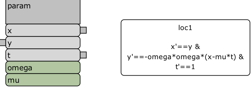
Base Component - Sine. For the sinusoid, we only need one base component that we call sin.
We have one location, named loc1, with three variables , , and . Using the equation 1, the flow is given by111Note that we opt for instead of to avoid any unexpected error caused by the SpacEx parser.
The three variables , , are declared as controlled, while the parameters / constants and are uncontrolled. The variable is a global variable, i.e. it can be communicated/shared to other components, whereas and are local variables. The hybrid automaton requires no invariant, reset, guard or synchronization label. Detailed information about modeling hybrid automata in SpaceEx can be found at [2]. The complete base component is shown in Figure 1.
The initial conditions are selected according to Section 2 to match the desired behavior of the sinusoidal signal.
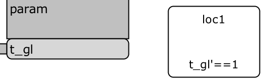
Base Component - Clock. We also need a base component that measures the global time. The name of the base component is clock and it has one variable . The variable is controlled and non-local. The base component has only one location with flow . The base component is portrayed in Figure 2.
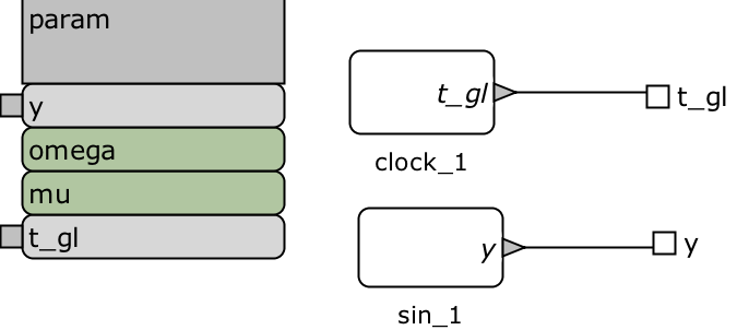
Network Component. For testing purposes, we add a network component that is a network of two hybrid automata. To do so, we add two binds in the Model Editor. The user can select the values of the parameters and here. The network component is portrayed in Figure 3.
4 Application
In this section, we show the applicability of this transformation via a numerical example as well as its usability within Simulink.
4.1 Numerical Example
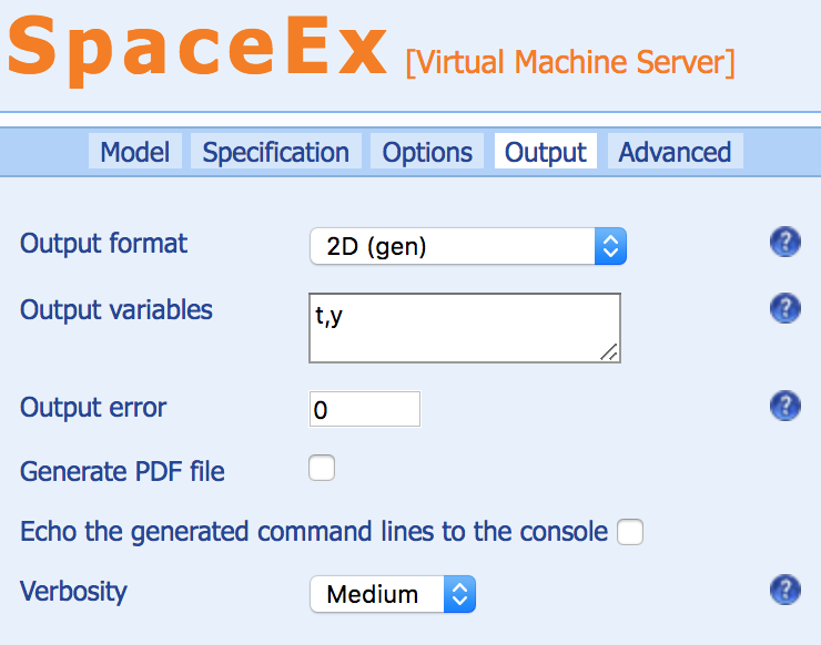
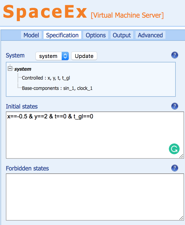
Consider that we opt for , , , and . After loading the model in the web interface, we need to select the initial states and the output variables. Note that , , and . For SpaceEx use, the output variables are defined in the Output tab, see Figure 4 and the initial states in the Specification tab, see Figure 5.
Then, we finalize the reachability analysis features in the Options tab by selecting the STC scenario, flowpipe tolerance 0.01, local time horizon 10s and max. iterations -1 (fixed point). The reachable set is shown in Figure 6.
4.2 Simulink sine wave block
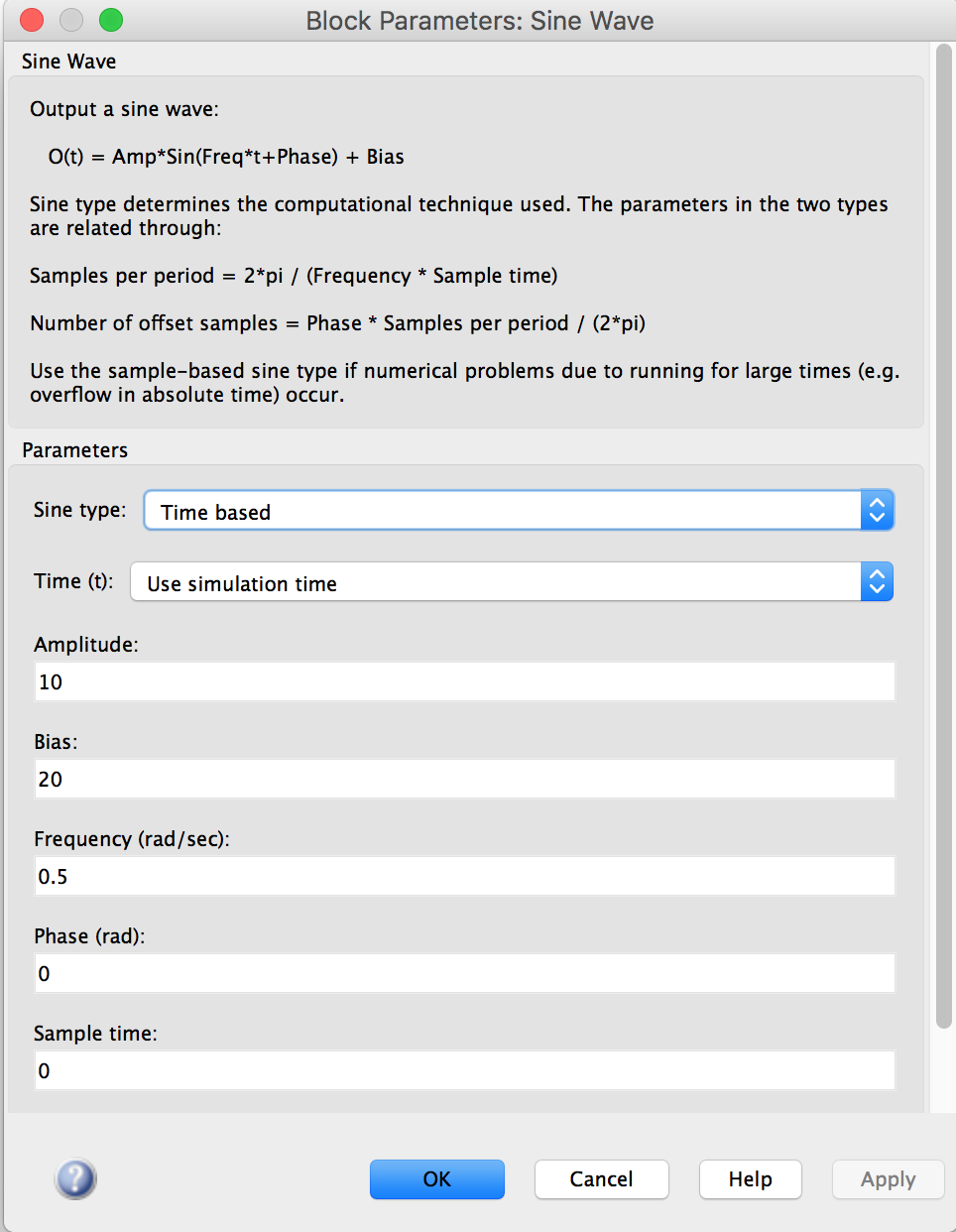
The proposed translation scheme is directly applicable to the Simulink sine wave block222https://www.mathworks.com/help/simulink/slref/sinewave.html. Figure 7 shows the options that exist in such a Simulink block. Table 1 presents the relation between the options in Simulink and the corresponding variables in SpaceEx. The translation of some Simulink blocks into hybrid automata supported by SpaceEx formalism is shown in [6, 5].
| Simulink | SpaceEx |
|---|---|
| Amplitude | |
| Bias | |
| Frequency | |
| Phase | |
| Sample time | – |
As it can be observed, the user can directly input the values of the Simulink block into the corresponding SpaceEx parameters. The initial conditions should be selected accordingly. Note that we shall opt the sampling time to be 0 as handle continuous-time systems.
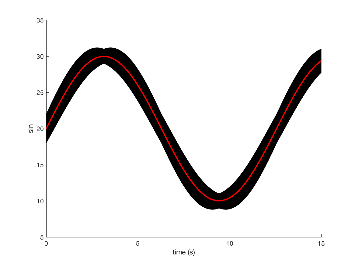
For the aforementioned example, we have , , , and . Then, and . Figure 8 shows the reachable set computed with SpaceEx against the Simulink simulation. The initial conditions are enlarged by 20% for the reachability computations. It can be observed that the simulation is included in the flowpipe.
References
- [1] Scott Cotton, Goran Frehse, and Olivier Lebeltel. The SpaceEx modeling language. http://spaceex.imag.fr/sites/default/files/spaceex_modeling_language_0.pdf, 2010.
- [2] Goran Frehse. An Introduction to SpaceEx v0.8. http://spaceex.imag.fr/documentation/user-documentation/introduction-spaceex-27, 2010.
- [3] Goran Frehse. An Introduction to Hybrid Automata, Numerical Simulation and Reachability Analysis. In Formal Modeling and Verification of Cyber-Physical Systems, pages 50–81. Springer, 2015.
- [4] Goran Frehse, Colas Le Guernic, Alexandre Donzé, Scott Cotton, Rajarshi Ray, Olivier Lebeltel, Rodolfo Ripado, Antoine Girard, Thao Dang, and Oded Maler. SpaceEx: Scalable verification of hybrid systems. In CAV Conference, 2011.
- [5] Nikolaos Kekatos. Formal Verification of Cyber-Physical Systems in the Industrial Model-Based Design Process. PhD thesis, 2018.
- [6] Nikolaos Kekatos, Marcelo Forets, and Goran Frehse. Constructing verification models of nonlinear simulink systems via syntactic hybridization. In 2017 IEEE 56th Annual Conference on Decision and Control (CDC), pages 1788–1795. IEEE, 2017.