End-to-End Annotator Bias Approximation
on Crowdsourced Single-Label Sentiment Analysis
Abstract
Sentiment analysis is often a crowdsourcing task prone to subjective labels given by many annotators. It is not yet fully understood how the annotation bias of each annotator can be modeled correctly with state-of-the-art methods. However, resolving annotator bias precisely and reliably is the key to understand annotators’ labeling behavior and to successfully resolve corresponding individual misconceptions and wrongdoings regarding the annotation task. Our contribution is an explanation and improvement for precise neural end-to-end bias modeling and ground truth estimation, which reduces an undesired mismatch in that regard of the existing state-of-the-art. Classification experiments show that it has potential to improve accuracy in cases where each sample is annotated only by one single annotator. We provide the whole source code publicly111https://github.com/theonlyandreas/end-to-end-crowdsourcing and release an own domain-specific sentiment dataset containing 10,000 sentences discussing organic food products222https://github.com/ghagerer/organic-dataset. These are crawled from social media and are singly labeled by 10 non-expert annotators.
1 Introduction
Modeling annotator bias in conditions where each data point is annotated by multiple annotators, below referred to as multi-labeled crowdsourcing, has been investigated thoroughly. However, bias modeling when every data point is annotated by only one person, hereafter called singly labeled crowdsourcing, poses a rather specific and difficult challenge. It is in particular relevant for sentiment analysis, where singly labeled crowdsourced datasets are prevalent. This is due to data from the social web which is annotated by the data creators themselves, e.g., rating reviewers or categorizing image uploaders. This might further include multi-media contents such as audio, video, images, and other forms of texts. While the outlook for such forms of data is promising, end-to-end approaches have not yet been fully explored on these types of crowdsourcing applications.
With these benefits in mind, we propose a neural network model tailored for such data with singly labeled crowdsourced annotations. It computes a latent truth for each sample and the correct bias of every annotator while also considering input feature distribution during training. We modify the loss function such that the annotator bias converges towards the actual confusion matrix of the regarding annotator and thus models the annotator biases correctly. This is novel, as previous methods either require a multi-labeled crowdsourcing setting Dawid and Skene (1979); Hovy et al. (2013) or do not produce a correct annotator bias during training which would equal the confusion matrix, see Zeng et al. (2018, figure 5) and Rodrigues and Pereira (2018, figure 3). A correct annotator- or annotator-group bias, however, is necessary to derive correct conclusions about the respective annotator behavior. This is especially important for highly unreliable annotators who label a high number of samples randomly – a setting, in which our proposed approach maintains its correctness, too.
Our contributions are as follows. We describe the corresponding state-of-the-art for crowdsourcing algorithms and tasks in section 2. Our neural network model method for end-to-end crowdsourcing modeling is explained in section 3, which includes a mathematical explanation that our linear bias modeling approach yields the actual confusion matrices. The experiments in section 4 underline our proof, show that the model handles annotator bias correctly as opposed to previous models, and demonstrate how the approach impacts classification.
2 Related Work
2.1 Crowdsourcing Algorithms
Problem definition. The need for data in the growing research areas of machine learning has given rise to the generalized use of crowdsourcing. This method of data collection increases the amount of data, saves time and money but comes at the potential cost of data quality. One of the key metrics of data quality is annotator reliability, which can be affected by various factors. For instance, the lack of rater accountability can entail spamming. Spammers are annotators that assign labels randomly and significantly reduce the quality of the data. Raykar and Yu (2012) and Hovy et al. (2013) addressed this issue by detecting spammers based on rater trustworthiness and the SpEM algorithm. However, spammers are not the only source of label inconsistencies. The varied personal backgrounds of crowd workers often lead to annotator biases that affect the overall accuracy of the models. Several works have previously ranked crowd workers Hovy et al. (2013); Whitehill et al. (2009); Yan et al. (2010), clustered annotators Peldszus and Stede (2013), captured sources of bias Wauthier and Jordan (2011) or modeled the varying difficulty of the annotation tasks Carpenter (2008); Whitehill et al. (2009); Welinder et al. (2010) allowing for the elimination of unreliable labels and the improvement of the model predictions.
Ground truth estimation. One common challenge in crowdsourced datasets is the ground truth estimation. When an instance has been annotated multiple times, a simple yet effective technique is to implement majority voting or an extension thereof TIAN and Zhu (2015); Yan et al. (2010). More sophisticated methods focus on modeling label uncertainty Spiegelhalter and Stovin (1983) or implementing bias correction Snow et al. (2008); Camilleri and Williams (2020). These techniques are commonly used for NLP applications or computer vision tasks Smyth et al. (1995); Camilleri and Williams (2020). Most of these methods for inferring the ground truth labels use variations of the EM algorithm by Dawid and Skene (1979), which estimates annotator biases and latent labels in turns. We use its recent extension called the Fast Dawid-Skene algorithm Sinha et al. (2018).
End-to-end approaches. The Dawid-Skene algorithm models the raters’ abilities as respective bias matrices. Similar examples include GLAD Whitehill et al. (2009) or MACE Hovy et al. (2013), which infer true labels as well as labeler expertise and sample difficulty. These approaches infer the ground truth only from the labels and do not consider the input features. End-to-end approaches learn a latent truth, annotator information, and feature distribution jointly during actual model training Zeng et al. (2018); Khetan et al. (2017); Rodrigues and Pereira (2018). Some works use the EM algorithm Raykar et al. (2009), e.g., to learn sample difficulties, annotator representations and ground truth estimates Platanios et al. (2020). However, the EM algorithm has drawbacks, namely that it can be unstable and more expensive to train Chu et al. (2020). LTNet models imperfect annotations derived from various image datasets using a single latent truth neural network and dataset-specific bias matrices Zeng et al. (2018). A similar approach is used for crowdsourcing, representing annotator bias by confusion matrix estimates Rodrigues and Pereira (2018). Both approaches show a mismatch between the bias and how it is modeled, see Zeng et al. (2018, figure 5) and Rodrigues and Pereira (2018, figure 3). We adapt the LTNet architecture (see section 3), as it can be used to model crowd annotators on singly labeled sentiment analysis, which, to our knowledge, is not done yet in the context of annotator bias modeling. Recent works about noisy labeling in sentiment analysis do not consider annotator bias Wang et al. (2019).
2.2 Crowdsourced Sentiment Datasets
Sentiment and Emotion. Many works use the terms sentiment and emotion interchangeably Demszky et al. (2020); Kossaifi et al. (2021), whereas sentiment is directed towards an entity Munezero et al. (2014) but emotion not necessarily. Both can be mapped to valence, which is the affective quality of goodness (high) or badness (low). Since emotion recognition often lacks annotated data, crowdsourced sentiment annotations can be beneficial Snow et al. (2008).
Multi-Labeled Crowdsourced Datasets. Crowdsourced datasets, such as, Google GoEmotion Demszky et al. (2020) and the SEWA database Kossaifi et al. (2021), usually contain multiple labels per sample and require their aggregation using ground truth estimation. Multi-labeled datasets are preferable to singly labeled ones on limited data. Snow et al. (2008) proved that many non-expert annotators give a better performance than a few expert annotators and are cheaper in comparison.
Singly Labeled Crowdsourced Datasets. Singly labeled datasets are an option given a fixed budget and unlimited data. Khetan et al. (2017) showed that it is possible to model worker quality with single labels even when the annotations are made by non-experts. Thus, multiple annotations can not only be redundant but come at the expense of fewer labeled samples. For singly labeled data, it can be distinguished between reviewer annotators and external annotators. Reviewer annotators rate samples they created themselves. It is common in forums for product and opinion reviews where a review is accompanied by a rating. As an example of this, we utilized the TripAdvisor dataset Thelwall (2018). Further candidates are the Amazon review dataset Ni et al. (2019), the Large Movie Review Dataset Maas et al. (2011), and many more comprising sentiment. External annotators annotate samples they have not created. Experts are needed for complex annotation tasks requiring domain knowledge. These are not crowdsourced, since the number of annotators is small and fixed. More common are external non-experts. Snow et al. (2008) showed that multi-labeled datasets annotated by non-expert improve performance. Khetan et al. (2017) showed that it also performs well in the singly labeled case. Thus, datasets made of singly labeled non-expert annotations can be cheaper, faster, and obtain performances comparable to those comprised of different types of annotations. Our organic dataset is annotated accordingly, see section 4.3.
3 Methodology
3.1 Basic Modeling Architecture
The model choice is determined by the fact that some of our datasets are small. Thus, the model should have only few trainable parameters to avoid overfitting. We utilize a simple attention mechanism, as it is comon for NLP applications. The input words are mapped to their word embeddings with , and being the input sequence length and the dimensionality of the input word vectors. These are GloVe embeddings of 50 dimensions pre-trained on 6B English tokens of the ”Wikipedia 2014 + Gigaword 5” dataset Pennington et al. (2014). Then, it computes the attention of each word using the trainable attention vector via . It takes the accordingly weighted average of the word vectors with denoting the -th sample or input text.
Finally, the classification head is the sigmoid of a simple linear layer , with and as the weights of the model. We refer to this last layer and to as latent truth layer or latent truth.
3.2 End-to-End Crowdsourcing Model
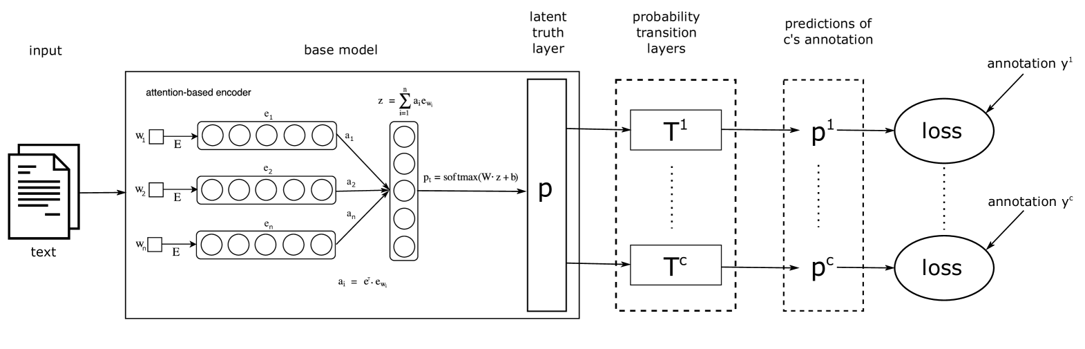
On top of the basic modeling architecture, the biases of the annotators are modeled as seen in figure 1. The theory is explained by Zeng et al. (2018) as follows:
“The labeling preference bias of different annotators cause inconsistent annotations. Each annotator has a coder-specific bias in assigning the samples to some categories. Mathematically speaking, let denote the data, the regarding annotations by coder . Inconsistent annotations assume that , where denotes the probability distribution that coder annotates sample . LTNet assumes that each sample has a latent truth . Without the loss of generality, let us suppose that LTNet classifies into the category with probability , where denotes the network parameters. If has a ground truth of , coder has an opportunity of to annotate as , where is the annotation of sample by coder . Then, the sample is annotated as label by coder with a probability of , where is the number of categories and
. denotes the transition matrix (also referred to as annotator bias) with rows summed to while is modeled by the base network Zeng et al. (2018). We define . Given the annotations from different coders on the data, LTNet aims to maximize the log-likelihood of the observed annotations. Therefore, parameters in LTNet are learned by minimizing the cross entropy loss of the predicted and observed annotations for each coder . ”
We represent the annotations and predictions as vectors of dimensionality such that is one-hot encoded and contains the probabilities for all class predictions of sample . The cross entropy loss function is then defined as .
3.3 The Effect of Logarithm Removal on Cross Entropy
The logarithm in the cross entropy formula leads to an exponential increase in the loss for false negative predictions, i.e., when the predicted probability for a ground truth class is close to and is . This increase can be helpful in conditions with numerical underflow, but at the same time this introduces a disproportionate high loss of the other class due to constantly misclassified items. This happens in crowdsourcing, for example, when one annotator is a spammer assigning a high degree of random annotations, which in turn leads to a disproportionally higher loss caused by that annotator’s many indistinguishable false negative annotations. Consequentially, the bias matrix of that annotator would be biased towards the false classes. Moreover, this annotator would cause overall more loss than other annotators, which can harm the model training for layers which are shared among all annotators, e.g., the latent truth layer when it is actually trained.
By omitting the log function, these effects are removed and all annotators and datapoints contribute with the same weight to the overall gradient and to the trainable annotator bias matrices, independent of the annotator and his respective annotation behavior. As a consequence, the annotator matrices are capable of modeling the real annotator bias, which is the mismatch between an annotation of coder and the latent truth prediction . If is one-hot encoded, this results to the according classification ratios of samples and is equal to the confusion matrix, without an algorithmically encoded bias towards a certain group of items. This is shown mathematically in the following, where it is assumed that the base network is fixed, i.e., backpropagation is performed through the bias matrices and stops at the latent truth layer.
We define as the number of all samples and of class . is the number of classes, the bias matrix of coder , the latent truth vector of sample , and the annotator prediction. is the latent truth of the -th sample of class with , same for and . The loss without logarithm is
Apparently, the derivation step between the second and third line would not work if there would be the logarithm from the standard cross entropy. Now, let the learning rate be , the number of epochs and the starting values of the initialized bias matrix . The bias parameters of the bias matrix are updated according to
For sufficiently large the starting values become infinitesimally small in comparison to the second additive term and thus negligible. As we are normalizing the rows of after training so that the bias fulfills our probability constraint defined in section 3.2, the linear factor is canceled out, too. Thus, the bias matrix results in the row normalized version of . is the sum of the latent truth probabilities for class on all samples of a ground truth class . If we assume that the latent truth is one hot encoded, equals to the confusion matrix, of which the -th column sums up to the number of samples in class : .
4 Experiments
4.1 Bias Convergence
The following experiment compares how training with and without the logarithm in the cross entropy loss affects the LTNet bias matrices empirically. The mathematical explanations in section 3.3 suggest that the logarithm removal from cross entropy leads to an annotator bias matrix identical to the confusion matrix, which would not be the case for the normal cross entropy.
Experiment Description. For the data, we use the TripAdvisor dataset from Thelwall et al. consisting of English consumer reviews about hotels from male and female reviewers plus their self-assigned sentiment ratings Thelwall (2018). We use the gender information to split the data into two annotator groups, male and female, from which we model each one with a corresponding bias matrix. We exclude neutral ratings and binarize the rest to be either positive or negative. As the dataset is by default completely balanced regarding gender and sentiment at each rating level, it is a natural candidate for correct bias approximation. Throughout our experiments, we use 70% of the obtained data as training, 20% as validation and the 10% remaining as test sets.
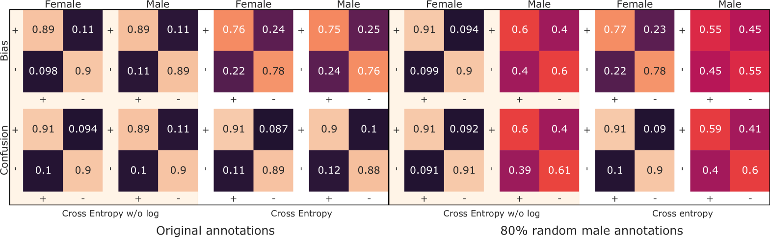
Similar to the explanation in 3.3, the base model with its latent truth predictions is pre-trained on all samples and then frozen when the bias matrices are trained. The stochastic gradient descent method is used to optimize the parameters, as other wide-spread optimizers, such as Adam and AdaGrad (the latter introduced that feature first), introduce an – in our case undesired – bias towards certain directions in the gradient space, namely by using the previous learning steps to increase or decrease the weights along dimensions with larger or smaller gradients Kingma and Ba (2014). For all four sub-experiments, we train the base models with varying hyperparameters and pick the best based on accuracy. We train the transition matrices 50 times with different learning rates from the interval . The batch size is 64. In addition to a normal training setting, we add random annotations to 80% of the instances annotated by male subjects, such that 40% from them are wrongly annotated. This results in four models: with and without logarithm in the cross entropy, with and without random male annotations, each time respectively with two annotator group matrices, male and female – see figure 2.
Results. The bias matrices of the models with the best accuracy are picked and presented in figure 2 in the top row. The corresponding confusion matrices depict the mismatch between latent truth predictions and annotator-group labels in the bottom row. The bias matrices trained without logarithm in the cross entropy are almost identical to the confusion matrices in all cases, which never holds for the normal cross entropy. This confirms our mathematically justified hypothesis given in section 3.3 that the logarithm removal from cross entropy leads to a correctly end-to-end-trained bias. In this context, it is relevant that the related work shows the same mismatch between bias and confusion matrix when applying cross entropy loss without explaining nor tackling this difference, see Zeng et al. (2018, figure 5) and Rodrigues and Pereira (2018, figure 3).
It is worth mentioning for the 80% random male annotations that these are correctly modeled without cross entropy, too, as opposed to normal cross entropy. If the goal is to model the annotator bias correctly in an end-to-end manner, this might be considered as particularly useful to analyze annotator behavior, e.g., spammer detection, later on.
Finally, we report how much variation the bias matrices show during training for cross entropy with and without logarithm. As mentioned in the experiment description, we trained each model times. The elements of the resulting bias matrices with standard cross entropy have on average standard deviation compared to without logarithm. It can be concluded that the bias produced by standard cross entropy is less stable during training, which raises questions about the overall reliability of its outcome.
In summary, the observations confirm our assumptions that cross entropy without logarithm captures annotator bias correctly in contrast to standard cross entropy. This carries the potential to detect spammer annotators and leads to an overall more stable training.
4.2 Ground Truth Estimation
In the following paragraphs, we demonstrate how to estimate the ground truth based on the latent truth from LTNet. This is then compared to two other kinds of ground truth estimates. All of them can be applied in a single label crowdsourcing setting.
The Dawid-Skene algorithm Sinha et al. (2018) is a common approach to calculate a ground truth in crowdsourcing settings where there are multiple annotations given on each sample. This method is, for instance, comparable to majority voting, which tends to give similar results for ground truth estimation. However, in single label crowdsourcing settings, these approaches are not feasible. Under single label conditions, the Dawid-Skene ground truth estimates equal to the single label annotations.
This is given by Sinha et al. (2018, formula 1) in the expectation step, where the probability for a class given the annotations is defined as
Here, is the sample to be estimated, the number of annotators for that sample, the set of annotators who labeled this sample, the set of annotation choices chosen by these participants for sample n, and the correct (or aggregated) label to be estimated for the sample Sinha et al. (2018).
In the single label case equals to 1, which reduces the formula to . This in turn equals to if is the assigned class label to sample by annotator , or otherwise. In other words, if there is only one annotation per sample, this annotation defines the ground truth. Since different annotators do not assign labels on the same samples, there is also no way to model mutual dependencies of each other.
LTNet, however, provides estimates for all variables from this formula. is the prior and is approximated by the latent truth probability for class of sample . is the probability that, assuming would be the given class, sample is labeled as by annotator . This equals to , i.e., the entries of the LTNet bias matrix of annotator .
Eventually, the LTNet ground truth can be derived by choosing such that the probability is maximized:
We will leverage this formula to derive and evaluate the ground truth generated by LTNet.
Experiment
We calculate the LTNet ground truth according to the previous formula on the organic dataset, a singly labeled crowdsourcing dataset, which is described in Section 4.3. To demonstrate the feasibility and the soundness of the approach, we compare it with two other ways of deriving a ground truth. Firstly, we apply the fast Dawid-Skene algorithm on the annotator-wise class predictions from the LTNet model. Secondly, we train a base network on all annotations while ignoring which annotator annotated which samples. Eventually, we compare the ground truth estimates of all three methods by calculating Cohen’s kappa coefficient Cohen (1960), which is a commonly used standard to analyze correspondence of annotations between two annotators or pseudo annotators. The training procedures and the dataset are identical to the ones from the classification experiments in Section 4.3.
Results
As can be seen on Table 1, the three ground truth estimators are all highly correlated to each other, since the minimal Cohen’s kappa score is . Apparently, there are only minor differences in the ground truth estimates, if any at all. Thus, it appears that the ground truths generated by the utilized methods are mostly identical. Especially, the LTNet and Dawid-Skene ground truths are highly correlated with a kappa of . The base model, which is completely unaware of which annotator labeled which sample, is slightly more distant with kappas between – . So with respect to the ground truth itself, we do not see a specific benefit of any method, since they are almost identical.
However, it must be noted that LTNet additionally produces correct bias matrices of every annotator during model training, which is not the case for the base model. Correct biases have the potential to help improving model performance by analyzing which annotators tend to be more problematic and weighting them accordingly.
| Dawid | Basic | ||
| Ground truths | Skene | LTNet | Model |
| Dawid Skene | |||
| LTNet | |||
| Base Model |
4.3 Classification
We conduct classification comparing LTNet in different configurations on three datasets with crowdsourced sentiment annotations to discuss the potential related benefits and drawbacks of our proposed loss modification.
Emotion Dataset. The emotion dataset consists of 100 headlines and their ratings for valence by multiple paid Amazon Mechanical Turk annotators Snow et al. (2008). Each headline is annotated by 10 annotators, and each annotated several but not all headlines. We split the interval-based valence annotations to positive, neutral, or negative. Throughout our experiments, we used 70% of the obtained data as training, 20% as validation and 10% as test sets.
Organic Food Dataset. With this paper, we publish our dataset containing social media texts discussing organic food related topics.
Source. The dataset was crawled in late 2017 from Quora, a social question-and-answer website. To retrieve relevant articles from the platform, the search terms ”organic”, ”organic food”, ”organic agriculture”, and ”organic farming” are used. The texts are deemed relevant by a domain expert if articles and comments deal with organic food or agriculture and discuss the characteristics, advantages, and disadvantages of organic food production and consumption. From the filtered data, 1,373 comments are chosen and 10,439 sentences annotated.
Annotation Scheme. Each sentence has sentiment (positive, negative, neutral) and entity, the sentiment target, annotated. We isolate sentiments expressed about organic against non-organic entities, whereas for classification only singly labeled samples annotated as organic entity are considered. Consumers discuss organic or non-organic products, farming practices, and companies.
Annotation Procedure. The data is annotated by each of the 10 coders separately; it is divided into 10 batches of sentences for each annotator and none of these batches shared any sentences between each other. 4616 sentences contain organic entities with 39% neutral, 32% positive, and 29% negative sentiments. After annotation, the data splits are 80% training, 10% validation, and 10% test set. The data distribution over sentiments, entities, and attributes remains similar on all splits.
Experiment Description. The experiment is conducted on the TripAdvisor, organic, and emotion datasets introduced in section 4.3. We compare the classification of the base network with three different LTNet configurations. Two of them are trained using cross entropy with and without logarithm. For the emotion dataset, we compute the bias matrices and the ground truth for the base model using the fast Dawid-Skene algorithm Sinha et al. (2018). This is possible for the emotion dataset, since each sample is annotated by several annotators.
We apply pre-training for each dataset by training several base models with different hyperparameters and pick the best based on accuracy. Eventually, we train the LTNet model on the crowdsourcing annotation targets by fine-tuning the best base model together with the bias matrices for the respective annotators. The bias matrices are initialized as row normalized identity matrices plus uniform noise around . The models are trained 50 times with varying learning rates sampled from between . A batch size of 64 is used.
| Dataset | Model | F1 % | Acc % |
| TripAdvisor | Base Model | 88.92 | 88.91 |
| LTNet w/o log | 89.71 | 89.71 | |
| LTNet | 89.39 | 89.39 | |
| Organic | Base Model | 32.08 | 45.75 |
| LTNet w/o log | 44.71 | 50.54 | |
| LTNet | 40.51 | 47.77 | |
| Emotion | Base Model | 51.74 | 56.00 |
| LTNet w/o log | 58.15 | 63.00 | |
| LTNet | 61.23 | 66.00 | |
| Base Model DS | 44.17 | 54.00 |
Results. The classification results of the models are presented in table 2 with their macro F1 score and accuracy as derived via predictions on the test sets. LTNet generally shows a significant classification advantage over the base model. On all three databases, LTNet approaches performed better on the test datasets. The LTNet improvement has a big delta of when there is a low annotation reliability (organic and emotion datasets) and a small delta with high reliability (TripAdvisor) 333Unreliable means that the provided annotations have a low Cohen’s kappa inter-rater reliability on the organic and emotion () dataset. On the organic dataset we prepared a separate data partition of 300 sentences annotated by all annotators for that purpose. For the TripAdvisor dataset, it is apparent that the correspondence of annotations between the two annotator groups (male and female) is high as can be seen in figure 2 for cross entropy without logarithm.. Apparently, model each annotator separately gives significant advantages.
Regarding the comparison between cross entropy (CE) loss with and without logarithm on LTNet, the removed logarithm shows better classification results on organic () and TripAdvisor data () and worse on the emotion dataset (). This means that on both of the singly labeled crowdsourcing datasets, the removal of the logarithm from the loss function leads to better predictions than the standard CE loss. On the multi-labeled emotion dataset, however, this does not appear to be beneficial. As this data has only a very small test set of 100 samples, it is not clear if this result is an artifact or not. Concluding, the log removal appears to be beneficial on large datasets, where the bias is correctly represented in the training and test data splits, such that it can be modeled correctly by the denoted approach. It shall be noted, that it is not clear if that observation would hold generally. We advice to run the same experiments multiple times on many more datasets to substantiate this finding.
5 Conclusion
We showed the efficacy of LTNet for modeling crowdsourced data and the inherent bias accurately and robustly. The bias matrices produced by our modified LTNet improve such that they are more similar to the actual bias between the latent truth and ground truth. Moreover, the produced bias shows high robustness under very noisy conditions making the approach potentially usable outside of lab conditions. The latent truth, which is a hidden layer below all annotator biases, can be used for ground truth estimation in our single label crowdsourcing scenario, providing almost identical ground truth estimates as pseudo labeling. Classification on three crowdsourced datasets show that LTNet approaches outperfom naive approaches not considering each annotator separately. The proposed log removal from the loss function showed better results on singly labeled crowdsourced datasets, but this observation needs further experiments to be substantiated. Furthermore, there might be many use cases to explore the approach on other tasks than sentiment analysis.
References
- Camilleri and Williams (2020) Michael P. J. Camilleri and Christopher K. I. Williams. 2020. The extended dawid-skene model. In Machine Learning and Knowledge Discovery in Databases, pages 121–136, Cham. Springer International Publishing.
- Carpenter (2008) Bob Carpenter. 2008. Multilevel bayesian models of categorical data annotation.
- Chu et al. (2020) Zhendong Chu, Jing Ma, and Hongning Wang. 2020. Learning from crowds by modeling common confusions.
- Cohen (1960) Jacob Cohen. 1960. A coefficient of agreement for nominal scales. Educational and psychological measurement, 20(1):37–46.
- Dawid and Skene (1979) A. P. Dawid and A. M. Skene. 1979. Maximum likelihood estimation of observer error-rates using the em algorithm. Applied Statistics, 28(1):20–28.
- Demszky et al. (2020) Dorottya Demszky, Dana Movshovitz-Attias, Jeongwoo Ko, Alan Cowen, Gaurav Nemade, and Sujith Ravi. 2020. Goemotions: A dataset of fine-grained emotions.
- He et al. (2017) Ruidan He, Wee Sun Lee, Hwee Tou Ng, and Daniel Dahlmeier. 2017. An unsupervised neural attention model for aspect extraction. In Proceedings of the 55th Annual Meeting of the Association for Computational Linguistics (Volume 1: Long Papers), pages 388–397, Vancouver, Canada. Association for Computational Linguistics.
- Hovy et al. (2013) Dirk Hovy, Taylor Berg-Kirkpatrick, Ashish Vaswani, and Eduard Hovy. 2013. Learning whom to trust with MACE. In Proceedings of the 2013 Conference of the North American Chapter of the Association for Computational Linguistics: Human Language Technologies, Atlanta, Georgia. Association for Computational Linguistics.
- Khetan et al. (2017) Ashish Khetan, Zachary C. Lipton, and Anima Anandkumar. 2017. Learning from noisy singly-labeled data.
- Kingma and Ba (2014) Diederik P. Kingma and Jimmy Ba. 2014. Adam: A method for stochastic optimization. CoRR, abs/1412.6980.
- Kossaifi et al. (2021) J. Kossaifi, R. Walecki, Y. Panagakis, J. Shen, M. Schmitt, F. Ringeval, J. Han, V. Pandit, A. Toisoul, B. Schuller, K. Star, E. Hajiyev, and M. Pantic. 2021. Sewa db: A rich database for audio-visual emotion and sentiment research in the wild. IEEE Transactions on Pattern Analysis and Machine Intelligence, 43(3):1022–1040.
- Maas et al. (2011) Andrew L. Maas, Raymond E. Daly, Peter T. Pham, Dan Huang, Andrew Y. Ng, and Christopher Potts. 2011. Learning word vectors for sentiment analysis. In Proceedings of the 49th Annual Meeting of the Association for Computational Linguistics: Human Language Technologies, Portland, Oregon, USA. Association for Computational Linguistics.
- Munezero et al. (2014) M. Munezero, C. S. Montero, E. Sutinen, and J. Pajunen. 2014. Are they different? affect, feeling, emotion, sentiment, and opinion detection in text. IEEE Transactions on Affective Computing, 5(2):101–111.
- Ni et al. (2019) Jianmo Ni, Jiacheng Li, and Julian McAuley. 2019. Justifying recommendations using distantly-labeled reviews and fine-grained aspects. In Proceedings of the 2019 Conference on Empirical Methods in Natural Language Processing and the 9th International Joint Conference on Natural Language Processing (EMNLP-IJCNLP), pages 188–197, Hong Kong, China. Association for Computational Linguistics.
- Peldszus and Stede (2013) Andreas Peldszus and Manfred Stede. 2013. Ranking the annotators: An agreement study on argumentation structure. In Proceedings of the 7th Linguistic Annotation Workshop and Interoperability with Discourse, pages 196–204, Sofia, Bulgaria. Association for Computational Linguistics.
- Pennington et al. (2014) Jeffrey Pennington, Richard Socher, and Christopher Manning. 2014. GloVe: Global vectors for word representation. In Proceedings of the 2014 Conference on Empirical Methods in Natural Language Processing (EMNLP), pages 1532–1543, Doha, Qatar. Association for Computational Linguistics.
- Platanios et al. (2020) Emmanouil Antonios Platanios, Maruan Al-Shedivat, Eric Xing, and Tom Mitchell. 2020. Learning from imperfect annotations.
- Raykar and Yu (2012) Vikas C. Raykar and Shipeng Yu. 2012. Eliminating spammers and ranking annotators for crowdsourced labeling tasks. J. Mach. Learn. Res., 13:491–518.
- Raykar et al. (2009) Vikas C. Raykar, Shipeng Yu, Linda H. Zhao, Anna K. Jerebko, Charles Florin, Gerardo Hermosillo Valadez, Luca Bogoni, and Linda Moy. 2009. Supervised learning from multiple experts: whom to trust when everyone lies a bit. In ICML, volume 382 of ACM International Conference Proceeding Series, pages 889–896. ACM.
- Rodrigues and Pereira (2018) Filipe Rodrigues and Francisco C. Pereira. 2018. Deep learning from crowds. Proceedings of the AAAI Conference on Artificial Intelligence, 32(1):1611–1618.
- Sinha et al. (2018) Vaibhav B Sinha, Sukrut Rao, and Vineeth N Balasubramanian. 2018. Fast dawid-skene: A fast vote aggregation scheme for sentiment classification.
- Smyth et al. (1995) Padhraic Smyth, Usama Fayyad, Michael Burl, Pietro Perona, and Pierre Baldi. 1995. Inferring ground truth from subjective labelling of venus images. In Advances in Neural Information Processing Systems, volume 7, pages 1085–1092, San Diego, CA. MIT Press.
- Snow et al. (2008) Rion Snow, Brendan O’Connor, Daniel Jurafsky, and Andrew Y. Ng. 2008. Cheap and fast—but is it good?: evaluating non-expert annotations for natural language tasks. In EMNLP ’08: Proceedings of the Conference on Empirical Methods in Natural Language Processing, Morristown, NJ, USA. Association for Computational Linguistics.
- Spiegelhalter and Stovin (1983) DJ Spiegelhalter and PGI Stovin. 1983. An analysis of repeated biopsies following cardiac transplantation. Statistics in medicine, 2(1):33–40.
- Thelwall (2018) Mike Thelwall. 2018. Gender bias in sentiment analysis. Online Information Review, 42(3):343–354.
- TIAN and Zhu (2015) TIAN TIAN and Jun Zhu. 2015. Max-margin majority voting for learning from crowds. In Advances in Neural Information Processing Systems, volume 28, pages 1621–1629, San Diego, CA. Curran Associates, Inc.
- Wang et al. (2019) Hao Wang, Bing Liu, Chaozhuo Li, Yan Yang, and Tianrui Li. 2019. Learning with noisy labels for sentence-level sentiment classification. CoRR, abs/1909.00124.
- Wauthier and Jordan (2011) Fabian L. Wauthier and Michael I. Jordan. 2011. Bayesian bias mitigation for crowdsourcing. In NIPS, volume 24, pages 1800–1808, San Diego, CA. Curran Associates, Inc.
- Welinder et al. (2010) Peter Welinder, Steve Branson, Serge Belongie, and Pietro Perona. 2010. The multidimensional wisdom of crowds. In Proceedings of the 23rd International Conference on Neural Information Processing Systems - Volume 2, Red Hook, NY, USA. Curran Associates Inc.
- Whitehill et al. (2009) Jacob Whitehill, Paul Ruvolo, Tingfan Wu, Jacob Bergsma, and Javier R. Movellan. 2009. Whose vote should count more: Optimal integration of labels from labelers of unknown expertise. In NIPS, pages 2035–2043, San Diego, CA. Curran Associates, Inc.
- Yan et al. (2010) Yan Yan, Rómer Rosales, Glenn Fung, Mark W. Schmidt, Gerardo Hermosillo Valadez, Luca Bogoni, Linda Moy, and Jennifer G. Dy. 2010. Modeling annotator expertise: Learning when everybody knows a bit of something. In AISTATS, volume 9 of JMLR Proceedings, pages 932–939, Chia Laguna Resort, Sardinia, Italy. JMLR.org.
- Zeng et al. (2018) Jiabei Zeng, Shiguang Shan, and Xilin Chen. 2018. Facial expression recognition with inconsistently annotated datasets. In ECCV (13), volume 11217 of Lecture Notes in Computer Science, pages 227–243, Red Hook, NY, USA. Springer.