End-to-End Segmentation via Patch-wise Polygons Prediction
Abstract
The leading segmentation methods represent the output map as a pixel grid. We study an alternative representation in which the object edges are modeled, per image patch, as a polygon with vertices that is coupled with per-patch label probabilities. The vertices are optimized by employing a differentiable neural renderer to create a raster image. The delineated region is then compared with the ground truth segmentation. Our method obtains multiple state-of-the-art results: 76.26% mIoU on the Cityscapes validation, 90.92% IoU on the Vaihingen building segmentation benchmark, 66.82% IoU for the MoNU microscopy dataset, and 90.91% for the bird benchmark CUB. Our code for training and reproducing these results is attached as supplementary.
1 Introduction
Accurate segmentation in dense environments is a challenging computer vision task. Many applications, such as autonomous driving [33], drone navigation [25], and human-robot interaction [24], rely on segmentation for performing scene understanding. Therefore, the accuracy of the segmentation method should be high as possible.
In recent years, fully convolutional networks based on encoder-decoder architectures [21], in which the encoder is pre-trained on ImageNet, have become the standard tool in the field. Several techniques were developed to better leverage the capacity of the architectures. For example, skip connections between the encoder and the decoder were added to overcome the loss of spatial information and to better propagate the training signal through the network [27]. What all these methods have in common is the representation of the output segmentation map as a binary multi-channel image, where the number of channels is the number of classes . In our work, we add a second type of output representation, in which, for every patch in the image and for every class, a polygon comprised of points represents the binary mask.
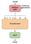
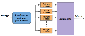
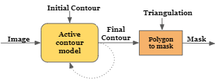
Alternative image segmentation architectures are presented in Fig. 1. The most common is the encoder-decoder one. The active contour methods, similar to our work, employ a polygon representation. Such methods, however, are iterative, and produce a single polygon, lacking the flexibility to cope with occlusions. Transformer based network employ patch-wise self-attention maps to calculate a spatial representation that attends globally to multiple parts of the image. The output mask is then generated by an MLP decoder. Our method differs from these approaches and produces multiple polygons, which are rendered by a neural renderer to produce the final segmentation mask.
For optimization purposes, we use a neural renderer to translate the polygons to a binary raster-graphics mask. The neural renderer provides a gradient for the polygon vertices and enables us to maximize the overlap between the output masks and the ground truth. Since there are polygons for every patch and every class, whether the object appears there or not, we multiply the binary mask with a low-resolution binary map that indicates the existence of each object.
The method achieves state-of-the-art results on four segmentation benchmarks, Cityscapes, CUB-200-2011, Nucleus segmentation challenges (MoNuSeg) and on the Vaihingen building segmentation benchmark.
 |
 |
|
| (a) | ||
 |
||
| (b) | (c) | (d) |
2 Related work
Most modern approaches to image segmentation perform image-to-image mapping with a Fully Convolutional Network [21]. Many encoder-decoder architectures were proposed, e.g., [12, 32, 30, 14], most of which employ U-Net based skip connections between parallel blocks of the encoder and the decoder [27]. Improved generalization is obtained by reducing the gap between the encoder and decoder semantic maps [41]. Another contribution adds residual connections for each encoder and decoder block and divides the image into patches with a calculated weighted map for each patch as input to the model. [37]. Wang et al. add attention maps to each feature map in the encoder-decoder block in order to enlarge the representation between far areas in the image with good computational efficiency [36]. This is extended by adding scalar gates to the attention layers [34]. The same contribution also adds a Local-Global training strategy (LoGo), which further improves performance. Dilated convolutions [38] are used by many methods to preserve the spatial size of the feature map and to enlarge the receptive field [5, 40, 39]. The receptive field can also be enlarged by using larger kernels [26] and enriched with contextual information, by using kernels of multiple scales [6]. Hardnet [4] employs a Harmonic Densely Connected Network that is shown to be highly effective in many real-time tasks, such as classification and object detection.
Polygon-based segmentation Active contour, also known as snakes [15], was used on many instance segmentation applications over the years. Such methods iteratively minimize an energy function that includes both edge-seeking terms and a shape prior until it stops [17, 8, 3]. The first deep learning-based snakes predict a correction vector for each point, by considering the small enclosing patch, in order to converge to the object outline [29]. Acuna et al.[1] propose automated and semi-automated methods for object annotating and segmentation based on Graph neural networks and reinforcement learning. Ling et al.[20] used a Graph Convolutional Network (GCN) in order to fit the polygon’s positions to the outline. A different approach predicts a shift map and iteratively changes the positions of the polygon vertices, according to this map [10]. In order to obtain a gradient signal, the authors use a neural renderer that transforms the 2D polygon into a 2D segmentation map. Our method also employs a neural renderer. However, we perform local predictions per patch and recover the vertex locations of the polygon in each patch non-iteratively. This allows us to perform finer local predictions, and overcome discontinuities caused by occlusions or by the existence of multiple objects.
A recent contribution [19], refines the output instance mask of pretrained Mask-RCNN algorithm by learning to correct the coordinates of the extracted polygons. This algorithm obtains good performances for the cityscapes instance segmentation benchmark but uses different settings than the rest of the literature. For example, the entire image is used instead of a specified bounding box, and the bounding box expansion differs from what is conventionally used in published work. Since no code was published, we cannot perform a direct comparison. From the algorithmic perspective, the methods greatly differ in the type of polygons used (boundary vs. local), the type of optimization (Chamfer Distance loss [13] on polygon coordinates vs. using a neural renderer), and almost every other aspect.
Neural Renderers The ground truth segmentation is given as an image, and in order to compare the obtained solution with it and compute a loss term, it is required to have a differentiable way to convert the vertex representation to a rasterized form. This conversion task, when implemented as a neural network, is referred to as “neural renderers”. On the backward pass, fully differential neural renderers convert image-based loss to gradients on the vertices’ coordinates. Loper et al. [22] approximate this gradient-based on image derivatives, while Kato et al. [16] approximates the propagated error, according to the overlap between the rasterization output and the ground truth.
 |
|
|
| (a) | (b) | (c) |
3 Methods
The input to our method is an RGB image , of dimensions . The image is divided into patches of size and a polygon with vertices is predicted for each patch. In addition, each patch has an associate scalar that determines the probability of the object being present in the patch.
This mask representation is illustrated in Fig. 2. The low-res probability map in panel (a) assigns one value per grid cell, where we denote higher probabilities by a brighter value. The local polygons in panel (b) determine a local segmentation mask in each grid cell. When the grid cell is completely enclosed by the segmented object, the polygon covers the entire cell. At object boundaries, it takes the form of the local boundary. When out of the object, it can degenerate to a zero area polygon or an arbitrary one. The final segmentation map, depicted in Fig. 2(c) is obtained by multiplying the low-resolution probability map with the local patch rastered for each polygon.
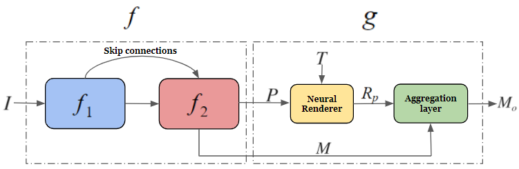
The learned network we employ is given as , where is the backbone (encoder) network, and is the decoder networks. The output space of is a tensor that can be viewed as a field with vectors , each representing a single polygon that is associated with a single image patch. This representation is the concatenation of the 2D coordinates of the vertices together with the probability. The image coordinates are normalized, such that their range is [-1,1].
 |
A fixed triangulation is obtained by performing Delaunay triangulation to a regular polygon of vertices. It is used to convert all polygons to a raster image, assuming that locally the polygons are almost always close to being convex. We set the z-axis to be constant and the perspective to be zero, in order to use a 3D renderer for 2D objects.
The output is divided into two parts, see Fig. 3. We denote by the set of all polygons, and by the map of size that contains all the probabilities. The neural renderer , given the vertices and the fixed triangulation , returns the polygon shape as a local image patch. In this raster image, all pixels inside the polygon defined by through the triangulation are assigned a value of one, zero for pixels outside, and in-between values for pixels that the polygon divides:
| (1) |
The aggregation layer collecting all local patches , each in its associated patch location, we obtain the map . By performing nearest neighbor upsampling to the probability map by a factor of in each dimension, and obtain a probability maps of the same size as . The final mask is the pixel-wise product between these two maps.
| (2) |
where denotes elementwise multiplication and denotes upsampling. This way, the low-resolution mask serves as a gating mechanism that determines whether the polygon exists within an object of a certain class in the output segmentation map.
To maximize the overlap between the output mask (before and after incorporating the polygons) and the ground truth segmentation map , a soft dice loss [31]:
| (3) |
Where TP is the true positive between the ground truth and output mask , FN is a false negative and FP is a false positive. In addition, a binary cross-entropy is used for :
| (4) |
| (5) |
This loss appears without weighting, in order to avoid an additional parameter. During inference, we employ only and the second term can be seen as auxiliary.
Architecture
For the backbone , the Harmonic Dense Net [4] is used, in which the receptive field is of size . The network contains six “HarD” blocks, as described in [4], with 192, 256, 320, 480, 720, 1280 output channels, respectively. The last block contains a dropout layer of 0.1. Pre-trained ImageNet weights are used at initialization.
The decoder contains two upsampling blocks in order to obtain an output resolution of times less than the original image size. Each block contains two convolutional layers with a kernel size equal to 3 and zero padding equal to one. In addition, we use batch normalization after the last convolution layer before the activation function. The first layer’s activation function is a ReLU, while the second layer’s activation functions are sigmoid for the channel of the low-resolution map and for the polygon vertices. Each layer receives a skip connection from the block of the encoder that has the same spatial resolution. We note that our decoder requires considerably fewer learnable parameters related to a regular decoder and, since only two blocks are used, fewer skip connections from the encoder.
The subsequent network employs the mesh renderer of [16], with a zero perspective, a camera distance of one, and output mask of size . This way, the 3D renderer is adapted for the 2D rendering task.
In term of FLOPs, for image size of we get 16.51 GMacs for our model and 25.44 GMacs for the comparable FCN. The peak memory consumption is 486MB for our model and 506MB for the FCN.
| Category | Full[train/val] | Occlusion[train/val] |
|---|---|---|
| Bicycle | 3501/1166 | 1029/385 |
| Bus | 374/98 | 115/30 |
| Car | 26226/4655 | 3333/914 |
| Person | 16753/3395 | 1731/669 |
| Train | 167/23 | 86/15 |
| Truck | 481/93 | 108/19 |
| Motorcycle | 707/149 | 175/55 |
| Rider | 1711/544 | 291/155 |
 |
|
|
|
 |
|
|
|
| (a) | (b) | (c) | (d) |
| Method | Bike | Bus | Person | Train | Truck | Mcycle | Car | Rider | Mean |
|---|---|---|---|---|---|---|---|---|---|
| Polygon-RNN++ (with BS) [1] | 63.06 | 81.38 | 72.41 | 64.28 | 78.90 | 62.01 | 79.08 | 69.95 | 71.38 |
| PSP-DeepLab [6] | 67.18 | 83.81 | 72.62 | 68.76 | 80.48 | 65.94 | 80.45 | 70.00 | 73.66 |
| Polygon-GCN (with PS) [20] | 66.55 | 85.01 | 72.94 | 60.99 | 79.78 | 63.87 | 81.09 | 71.00 | 72.66 |
| Spline-GCN (with PS) [20] | 67.36 | 85.43 | 73.72 | 64.40 | 80.22 | 64.86 | 81.88 | 71.73 | 73.70 |
| Ours | 68.20 | 85.10 | 74.52 | 74.80 | 80.50 | 66.20 | 82.10 | 71.81 | 75.40 |
| Deep contour [10] | 68.08 | 83.02 | 75.04 | 74.53 | 79.55 | 66.53 | 81.92 | 72.03 | 75.09 |
| FCN-HarDNet-85 [4] | 68.26 | 84.98 | 74.51 | 76.60 | 80.20 | 66.25 | 82.36 | 71.57 | 75.59 |
| Ours | 69.53 | 85.50 | 75.15 | 76.90 | 81.20 | 66.96 | 82.69 | 72.18 | 76.26 |
| Method | F1-Score | mIoU | WCov | FBound |
|---|---|---|---|---|
| FCN-UNet (Ronneberger 2015) | 87.40 | 78.60 | 81.80 | 40.20 |
| FCN-ResNet34 | 91.76 | 87.20 | 88.55 | 75.12 |
| FCN-HarDNet-85 (Chao 2019) | 93.97 | 88.95 | 93.60 | 80.20 |
| DSAC (Marcos 2018) | - | 71.10 | 70.70 | 36.40 |
| DarNet (Cheng 2019) | 93.66 | 88.20 | 88.10 | 75.90 |
| Deep contour (Gur 2019) | 94.80 | 90.33 | 93.72 | 78.72 |
| TDAC (Hatamizadeh 2020) | 94.26 | 89.16 | 90.54 | 78.12 |
| Ours | 95.15 | 90.92 | 94.36 | 83.89 |
 |
 |
 |
 |
 |
 |
 |
 |
| (a) | (b) | (c) | (d) |
| Method | Dice | mIoU |
|---|---|---|
| FCN [2] | 28.84 | 28.71 |
| U-Net [27] | 79.43 | 65.99 |
| U-Net++[41] | 79.49 | 66.04 |
| Res-UNet[37] | 79.49 | 66.07 |
| Axial Attention U-Net[36] | 76.83 | 62.49 |
| MedT[34] | 79.55 | 66.17 |
| FCN-Hardnet85 | 79.52 | 66.06 |
| Low res FCN-Hardnet85 () | 65.82 | 49.13 |
| Ours () | 80.05 | 66.82 |
 |
 |
 |
 |
 |
 |
 |
 |
 |
 |
 |
 |
| (a) | (b) | (c) | (d) |
4 Experiments
We present our results on three segmentation benchmarks and compare our performance with the state-of-the-art methods. We further perform a study on the effect of each parameter of the proposed algorithm, and on the effect of the underlying network architecture. We put an added emphasis on the subset of test images that depict an occlusion of the segmented object.
The Citycapes dataset [9] for instance segmentation includes eight object classes with fine-annotated images, divided into images for training, for validation, and for the test set.
The Cityscapes dataset contains urban scenes that are characterized by dense and multiple objects. In order to fully understand the scene, the segmentation method is required to be robust to occlusions of objects, which causes the segmentation task to be more challenging. Following [20], we train and evaluate given the bounding box of the object, such that the network outputs a single mask for the entire instance.
To analyze the images with occlusions, the cases where the ground truth contains at least two contours are identified. for this purpose, we define an occlusion distance per image as:
| (6) |
where is the set of all contours of a specific class defined for a specific image, each contour being a set of points. The distance , which degenerates to zero if there is only one contour, is then used to stratify the test images by the number of occlusions. Tab. 1 contains the number of images in both the validation set of the entire Cityscapes dataset, as well as for the subset of which the occlusion distance is larger than one. As can be seen, occlusions are fairly common for many of the objects.
The baseline methods we compare to on the Cityscapes dataset are PSPDeepLab[6], Polygon-RNN++[1], Curve-GCN[20] and Deep active contours [10]. Another baseline, denoted as “FCN-HarDNet-85” employs a fully-convolutional network with the same backbone [4] we used for our own method.
We note that our method employs 17M parameters in its decoder, while the “FCN-HarDNet-85” employs a decoder with 22M parameters.
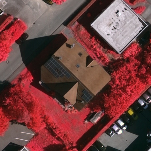
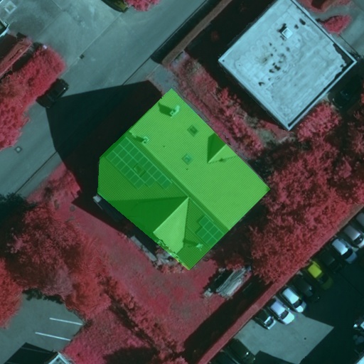
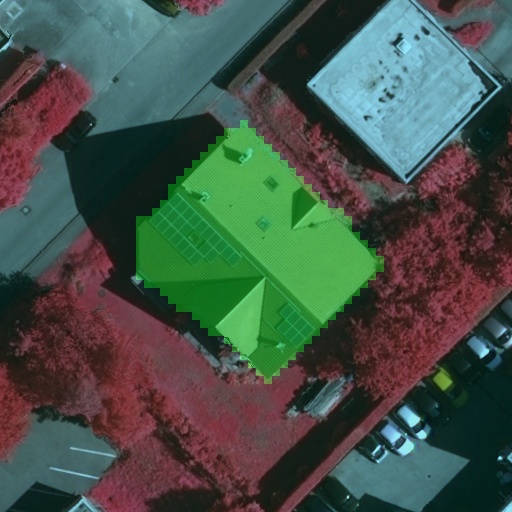
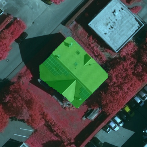
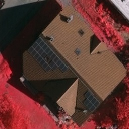
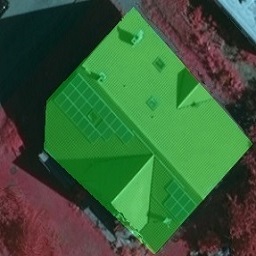
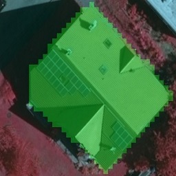
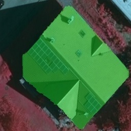
The Vaihingen [28] dataset consists of 168 aerial images, at a resolution of , from this German city. The task is to segment the central building in a very dense and challenging environment, which includes other structures, streets, trees, and cars. The dataset is divided into 100 buildings for training, and the remaining 68 for testing.
For building segmentation, we use an encoder-decoder architecture based on the HarDNet-85 [4] backbone and produce at 1/8 resolution ().
The baseline methods we compare to on the Vaihingen buildings dataset are “DSAC”[23], “DarNet”[7], “TDAC”[11] and Deep active contours [10]. We also present results for “FCN-UNET” [27], “FCN-ResNet-34” and “FCN-HarDNet-85”, all based on fully-convolutional network decoders.
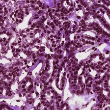
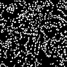
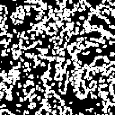
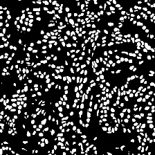
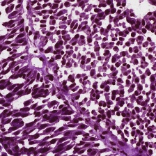
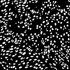
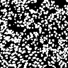
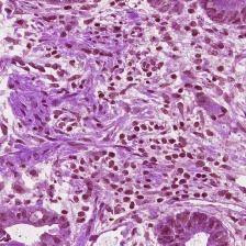
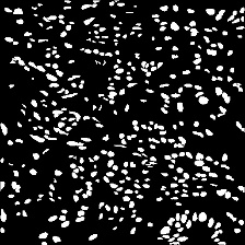
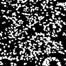
The MoNuSeg dataset [18] contains a training set with 30 microscopic images from seven organs with annotations of 21,623 individual nuclei, the test dataset contains 14 similar images. Following previous work, we resized the images into a resolution of [34]. An encoder-decoder architecture based on the HarDNet-85 [4] backbone. Since the recovered elements are very small, our method employs a map at 1/4 resolution (), and not lower resolutions as in other datasets.
The baseline methods we compare to on the Monu dataset are “FCN”[2], “UNET”[27], “UNET++”[41], Res-Unet[37], Axial attention Unet[36] and Medical transformer [34].
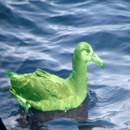
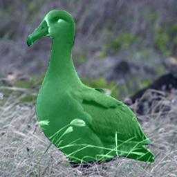
Finally, we report results on CUB-200-2011 [35]. The dataset contains 5994 images of different birds for training, and 5794 for validation. We trained the model for the same setting of cityscapes where the input image size is and the evaluation is on the original image size.
Training details For training our network, we use the ADAM optimizer with an initial learning rate of 0.0003 and a gamma decay of 0.7, applied every 50 epochs. The batch size is 32 and the parameter of the weight decay regularization is set to . A single GeForce RTX 2080 Ti is used for training on all datasets. Our networks are trained for up to 1000 epochs.
Following [10], we used for the Cityscapes images a set of augmentations that includes: (i) scaling by a random scale factor in the range of and then cropping an image of size , (ii) color jitter with the parameters of brightness sampled uniformly between , a contrast in the range , saturation in the range , and hue in the range , (iii) a random horizontal flip with a probability of 0.5.
For the Vaihingen dataset, also following [10], we used (i) a random rotation augmentation of 360 degrees and a scale range of , (ii) a random vertical and horizontal flip with a probability of 0.5, (iii) random color jitter with a maximal value of 0.6 for brightness, 0.5 for contrast, 0.4 for saturation, and 0.025 for hue.
For the MoNu dataset, we used (i) a random rotation augmentation of ±20 degrees and a scale range of , (ii) a random horizontal flip with a probability of 0.5, (iii) random color jitter with a maximal value of 0.4 for brightness, 0.4 for contrast, 0.4 for saturation, and 0.1 for hue.
Evaluation Metrics The Cityscapes segmentation results employ the common metrics of mean Intersection-over-Union (IoU). The Vaihingen benchmark is equipped with a set of additional evaluation metrics. The results are evaluation by the IoU of the single class, and the F1-score of retrieving building pixels. The weighted Coverage (WCov) score is computed as the IoU for each object in the image weighted by the related size of the object from the whole image. Finally, the Boundary F-score (BoundF) is the average of the F1-scores computed with thresholds ranging from 1 to 5 pixels around the ground truth boundaries, as described by [28].
Results The Cityscapes results are presented in Tab. 2. As can be seen, our method outperforms all baseline methods, including active contour methods and encoder-decoder architectures. Furthermore, one can observe the gap in performance between our method and the U-Net-like method that is based on the same backbone architecture (“FCN-HarDNet-85”). This is despite the reduction in the number of trainable parameters and the size of the representation (each patch is represented by output floats, instead of 64 floats).
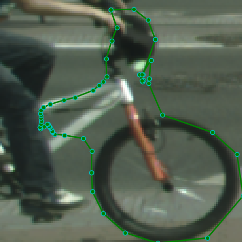
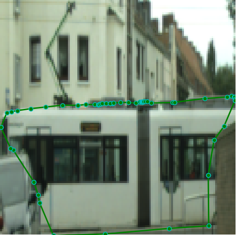
Fig. 4 presents sample results and compares our method to the leading active contour method (“Deep contour”) and to the FCN-HarDNet-85 baseline. As can be seen, the active contour method struggles to model objects that deviate considerably from their convex hull, and cannot handle occlusions well. In comparison to the FCN baseline, our method provides more accurate details (consider the bicycle fork in the first row), but the overall shape is the same.
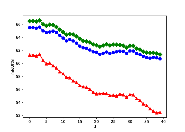
The results for images stratified by the level of occlusion (the measurement ) are presented in Fig. 5. All methods present a decrease in performance as the amount of occlusion increases. The FCN-HarDNet-85 maintains a stable performance level below our method, and the active contour method suffers the most from occlusion, as expected.
The results for the Vaihingen building dataset are presented in Tab. 3. Our method outperforms both the fully connected segmentation methods, as well as the active-contour based methods. Fig. 6 presents typical samples, demonstrating the refinement that is obtained by the polygons over the initial segmentation mask.
The results for MoNu dataset are reported in Tab. 4. We outperform all baselines for both the Dice score and mean-IoU. Our algorithm also obtains better performances in comparison to the fully convolutional segmentation network with the same backbone Hardnet-85. The improvement from low resolution mask () to the output mask () is from 49.13% IoU to 66.82%. The full resolution FCN-Hardnet85 obtains a lower result of 66.06 IoU. Fig. 7 presents the output mask of our algorithm for samples from the test set.
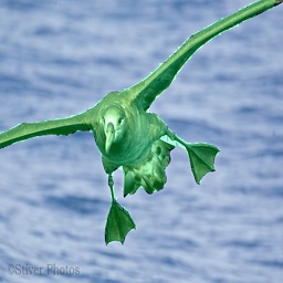
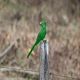
The results for CUB-200-2011 are reported in Tab. 5. We obtain better results than both FCN-Hardnet85 and Deep Contour on all metrics. Fig. 8 present the output mask of our algorithm for samples from CUB-200-2011.
| Method | Dice | mIoU | FBound |
|---|---|---|---|
| U-Net [27] | 93.84 | 88.80 | 76.54 |
| Deep contour [10] | 93.72 | 88.35 | 75.92 |
| FCN-Hardnet85 | 94.91 | 90.51 | 79.73 |
| Low res FCN-Hardnet85 () | 84.45 | 73.43 | 39.47 |
| Ours () | 95.11 | 90.91 | 79.86 |
|
|
 |
 |
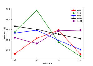
Parameter sensitivity The proposed patch-wise polygon scheme adds two hyperparameters: the size of the patch that each polygon for each class is applied to and the number of vertices in each polygon. In order to study the effect of these parameters, we varied the number of vertices to be in the range of and the size of the patch to be one of .
Fig. 9 shows our network performances for building segmentation, when varying the two parameters. As can be seen, for small patches, for instance, or , the number of nodes that optimizes performance is five. As may be expected, for larger patches, the method performs better with a higher number of vertices.
We also checked our performances for different Hardnet backbones - HarDNnet39DS, HarDNnet68DS, HarDNnet68, HarDNnet85 (DS stands for for depth-wise-separable, see [4]). The results appear in Tab. 6 for the building dataset. As expected, the performance improves with the increase in the number of parameters in the network. It can also be observed that the low- resolution mask after upsampling and the refined mask have a performance gap of 4% in terms of mean IoU, in favor of the latter, across all of the backbones.
| Backbone | Params[#] | [mIoU] | [mIoU] |
|---|---|---|---|
| HarDNet-39DS | 3.5M | 89.11 | 85.07 |
| HarDNet-68DS | 4.2M | 89.75 | 85.40 |
| HarDNet-68 | 17.6M | 90.50 | 85.60 |
| HarDNet-85 | 36.7M | 90.92 | 85.98 |
5 Discussion
The ability to work with polygons allows our network to produce segmentation maps at a resolution that is limited only by machine precision. This can be seen in Fig. 2(b), where the polygons have fractional coordinates. These polygons can be rasterized at any resolution.
The property of practically-infinite resolution may be of use in applications that require an adaptive resolution, depending on the object or its specific regions. An example is foreground segmentation for background replacement (virtual “green screens”), in which hair regions require finer resolutions. Such scenarios would raise research questions about training networks at a resolution that is higher than the resolution of the ground truth data, and on the proper evaluation of the obtained results.
We note that while we do not enforce the polygons of nearby patches to be compatible at the edges, this happens naturally, as can be seen in Fig. 2(b). Earlier during development, we have attempted to use loss terms that encourage such compatibility but did not observe an improvement.
Further inspection of the obtained polygons reveals that polygons with often employ overlapping vertices in order to match the square cell edges. In empty regions, polygons tend to become of zero-area by sticking to one of the boundaries. These behaviors emerge without being directly enforced. In some cases, phantom objects are detected by single polygons, as in the top right part of Fig. 2(b). These polygons are removed by the gating process that multiplies with , as can be seen in Fig. 2(c). We do not observe such polygons in the output images.
6 Conclusions
The pixel grid representation is commonly used by deep segmentation networks. In this work, we present an alternative approach that encodes the local segmentation maps as polygons. The method employs a neural renderer to backprop the rasterization process. A direct comparison to a method that employs the same backbone but without the polygonal representation reveals a significant improvement in performance on multiple benchmarks, despite using fewer training parameters. Moreover, our method also outperforms all other segmentation methods.
Acknowledgment
This project has received funding from the European Research Council (ERC) under the European Unions Horizon 2020 research and innovation programme (grant ERC CoG 725974).
References
- [1] David Acuna, Huan Ling, Amlan Kar, and Sanja Fidler. Efficient interactive annotation of segmentation datasets with polygon-rnn++. In Proceedings of the IEEE conference on Computer Vision and Pattern Recognition, pages 859–868, 2018.
- [2] Vijay Badrinarayanan, Alex Kendall, and Roberto Cipolla. Segnet: A deep convolutional encoder-decoder architecture for image segmentation. IEEE transactions on pattern analysis and machine intelligence, 39(12):2481–2495, 2017.
- [3] Vicent Caselles, Ron Kimmel, and Guillermo Sapiro. Geodesic active contours. International journal of computer vision, 22(1):61–79, 1997.
- [4] Ping Chao, Chao-Yang Kao, Yu-Shan Ruan, Chien-Hsiang Huang, and Youn-Long Lin. Hardnet: A low memory traffic network. In Proceedings of the IEEE International Conference on Computer Vision, pages 3552–3561, 2019.
- [5] Liang-Chieh Chen, George Papandreou, Iasonas Kokkinos, Kevin Murphy, and Alan L Yuille. Semantic image segmentation with deep convolutional nets and fully connected crfs. arXiv preprint arXiv:1412.7062, 2014.
- [6] Liang-Chieh Chen, George Papandreou, Iasonas Kokkinos, Kevin Murphy, and Alan L Yuille. Deeplab: Semantic image segmentation with deep convolutional nets, atrous convolution, and fully connected crfs. IEEE transactions on pattern analysis and machine intelligence, 40(4):834–848, 2017.
- [7] Dominic Cheng, Renjie Liao, Sanja Fidler, and Raquel Urtasun. Darnet: Deep active ray network for building segmentation. In Proceedings of the IEEE Conference on Computer Vision and Pattern Recognition, pages 7431–7439, 2019.
- [8] Laurent D Cohen. On active contour models and balloons. CVGIP: Image understanding, 53(2):211–218, 1991.
- [9] Marius Cordts, Mohamed Omran, Sebastian Ramos, Timo Rehfeld, Markus Enzweiler, Rodrigo Benenson, Uwe Franke, Stefan Roth, and Bernt Schiele. The cityscapes dataset for semantic urban scene understanding. In Proceedings of the IEEE conference on computer vision and pattern recognition, pages 3213–3223, 2016.
- [10] Shir Gur, Tal Shaharabany, and Lior Wolf. End to end trainable active contours via differentiable rendering. arXiv preprint arXiv:1912.00367, 2019.
- [11] Ali Hatamizadeh, Debleena Sengupta, and Demetri Terzopoulos. End-to-end trainable deep active contour models for automated image segmentation: Delineating buildings in aerial imagery. In European Conference on Computer Vision, pages 730–746. Springer, 2020.
- [12] Kaiming He, Xiangyu Zhang, Shaoqing Ren, and Jian Sun. Deep residual learning for image recognition. In Proceedings of the IEEE conference on computer vision and pattern recognition, pages 770–778, 2016.
- [13] Namdar Homayounfar, Wei-Chiu Ma, Shrinidhi Kowshika Lakshmikanth, and Raquel Urtasun. Hierarchical recurrent attention networks for structured online maps. In Proceedings of the IEEE Conference on Computer Vision and Pattern Recognition, pages 3417–3426, 2018.
- [14] Gao Huang, Zhuang Liu, Laurens Van Der Maaten, and Kilian Q Weinberger. Densely connected convolutional networks. In Proceedings of the IEEE conference on computer vision and pattern recognition, pages 4700–4708, 2017.
- [15] Michael Kass, Andrew Witkin, and Demetri Terzopoulos. Snakes: Active contour models. International journal of computer vision, 1(4):321–331, 1988.
- [16] Hiroharu Kato, Yoshitaka Ushiku, and Tatsuya Harada. Neural 3d mesh renderer. In Proceedings of the IEEE Conference on Computer Vision and Pattern Recognition, pages 3907–3916, 2018.
- [17] Satyanad Kichenassamy, Arun Kumar, Peter Olver, Allen Tannenbaum, and Anthony Yezzi. Gradient flows and geometric active contour models. In Proceedings of IEEE International Conference on Computer Vision, pages 810–815. IEEE, 1995.
- [18] Neeraj Kumar, Ruchika Verma, Deepak Anand, Yanning Zhou, Omer Fahri Onder, Efstratios Tsougenis, Hao Chen, Pheng-Ann Heng, Jiahui Li, Zhiqiang Hu, et al. A multi-organ nucleus segmentation challenge. IEEE transactions on medical imaging, 39(5):1380–1391, 2019.
- [19] Justin Liang, Namdar Homayounfar, Wei-Chiu Ma, Yuwen Xiong, Rui Hu, and Raquel Urtasun. Polytransform: Deep polygon transformer for instance segmentation. In Proceedings of the IEEE/CVF Conference on Computer Vision and Pattern Recognition, pages 9131–9140, 2020.
- [20] Huan Ling, Jun Gao, Amlan Kar, Wenzheng Chen, and Sanja Fidler. Fast interactive object annotation with curve-gcn. In Proceedings of the IEEE/CVF Conference on Computer Vision and Pattern Recognition, pages 5257–5266, 2019.
- [21] Jonathan Long, Evan Shelhamer, and Trevor Darrell. Fully convolutional networks for semantic segmentation. In Proceedings of the IEEE conference on computer vision and pattern recognition, pages 3431–3440, 2015.
- [22] Matthew M Loper and Michael J Black. Opendr: An approximate differentiable renderer. In European Conference on Computer Vision, pages 154–169. Springer, 2014.
- [23] Diego Marcos, Devis Tuia, Benjamin Kellenberger, Lisa Zhang, Min Bai, Renjie Liao, and Raquel Urtasun. Learning deep structured active contours end-to-end. In Proceedings of the IEEE Conference on Computer Vision and Pattern Recognition, pages 8877–8885, 2018.
- [24] Gabriel L Oliveira, Claas Bollen, Wolfram Burgard, and Thomas Brox. Efficient and robust deep networks for semantic segmentation. The International Journal of Robotics Research, 37(4-5):472–491, 2018.
- [25] Vivek Parmar, Narayani Bhatia, Shubham Negi, and Manan Suri. Exploration of optimized semantic segmentation architectures for edge-deployment on drones. arXiv preprint arXiv:2007.02839, 2020.
- [26] Chao Peng, Xiangyu Zhang, Gang Yu, Guiming Luo, and Jian Sun. Large kernel matters–improve semantic segmentation by global convolutional network. In Proceedings of the IEEE conference on computer vision and pattern recognition, pages 4353–4361, 2017.
- [27] Olaf Ronneberger, Philipp Fischer, and Thomas Brox. U-net: Convolutional networks for biomedical image segmentation. In International Conference on Medical image computing and computer-assisted intervention, pages 234–241. Springer, 2015.
- [28] Franz Rottensteiner, Gunho Sohn, Jaewook Jung, Markus Gerke, Caroline Baillard, Sébastien Bénitez, and U Breitkopf. International society for photogrammetry and remote sensing, 2d semantic labeling contest. http://www2.isprs.org/commissions/comm3/wg4/semantic-labeling.html.
- [29] Christian Rupprecht, Elizabeth Huaroc, Maximilian Baust, and Nassir Navab. Deep active contours. arXiv preprint arXiv:1607.05074, 2016.
- [30] Karen Simonyan and Andrew Zisserman. Very deep convolutional networks for large-scale image recognition. arXiv preprint arXiv:1409.1556, 2014.
- [31] Carole H Sudre, Wenqi Li, Tom Vercauteren, Sebastien Ourselin, and M Jorge Cardoso. Generalised dice overlap as a deep learning loss function for highly unbalanced segmentations. In Deep learning in medical image analysis and multimodal learning for clinical decision support, pages 240–248. Springer, 2017.
- [32] Christian Szegedy, Wei Liu, Yangqing Jia, Pierre Sermanet, Scott Reed, Dragomir Anguelov, Dumitru Erhan, Vincent Vanhoucke, and Andrew Rabinovich. Going deeper with convolutions. In Proceedings of the IEEE conference on computer vision and pattern recognition, pages 1–9, 2015.
- [33] Michael Treml, José Arjona-Medina, Thomas Unterthiner, Rupesh Durgesh, Felix Friedmann, Peter Schuberth, Andreas Mayr, Martin Heusel, Markus Hofmarcher, Michael Widrich, et al. Speeding up semantic segmentation for autonomous driving. In MLITS, NIPS Workshop, volume 2, 2016.
- [34] Jeya Maria Jose Valanarasu, Poojan Oza, Ilker Hacihaliloglu, and Vishal M Patel. Medical transformer: Gated axial-attention for medical image segmentation. arXiv preprint arXiv:2102.10662, 2021.
- [35] Catherine Wah, Steve Branson, Peter Welinder, Pietro Perona, and Serge Belongie. The Caltech-UCSD birds-200-2011 dataset. 2011.
- [36] Huiyu Wang, Yukun Zhu, Bradley Green, Hartwig Adam, Alan Yuille, and Liang-Chieh Chen. Axial-deeplab: Stand-alone axial-attention for panoptic segmentation. In European Conference on Computer Vision, pages 108–126. Springer, 2020.
- [37] Xiao Xiao, Shen Lian, Zhiming Luo, and Shaozi Li. Weighted res-unet for high-quality retina vessel segmentation. In 2018 9th international conference on information technology in medicine and education (ITME), pages 327–331. IEEE, 2018.
- [38] Fisher Yu and Vladlen Koltun. Multi-scale context aggregation by dilated convolutions. arXiv preprint arXiv:1511.07122, 2015.
- [39] Hang Zhang, Kristin Dana, Jianping Shi, Zhongyue Zhang, Xiaogang Wang, Ambrish Tyagi, and Amit Agrawal. Context encoding for semantic segmentation. In Proceedings of the IEEE conference on Computer Vision and Pattern Recognition, pages 7151–7160, 2018.
- [40] Hengshuang Zhao, Jianping Shi, Xiaojuan Qi, Xiaogang Wang, and Jiaya Jia. Pyramid scene parsing network. In Proceedings of the IEEE conference on computer vision and pattern recognition, pages 2881–2890, 2017.
- [41] Zongwei Zhou, Md Mahfuzur Rahman Siddiquee, Nima Tajbakhsh, and Jianming Liang. Unet++: A nested u-net architecture for medical image segmentation. In Deep learning in medical image analysis and multimodal learning for clinical decision support, pages 3–11. Springer, 2018.