This paper was converted on www.awesomepapers.org from LaTeX by an anonymous user.
Want to know more? Visit the Converter page.

Endogenous Stochastic Arbitrage Bubbles
and the Black–Scholes model.

Mauricio Contreras G Universidad Metropolitana de Ciencias de la Educación UMCE.      email: mauricio.contreras@umce.cl

This paper develops a model that incorporates the presence of stochastic arbitrage explicitly in the Black–Scholes equation. Here, the arbitrage is generated by a stochastic bubble, which generalizes the deterministic arbitrage model obtained in the literature [17]. It is considered to be a generic stochastic dynamic for the arbitrage bubble, and a generalized Black–Scholes equation is then derived. The resulting equation is similar to that of the stochastic volatility models, but there are no undetermined parameters as the market price of risk.
The proposed theory has asymptotic behaviors that are associated with the weak and strong arbitrage bubble limits. For the case where the arbitrage bubble’s volatility is zero (deterministic bubble), the weak limit corresponds to the usual Black-Scholes model. The strong limit case also give a Black–Scholes model, but the underlying asset’s mean value replaces the interest rate. When the bubble is stochastic, the theory also has weak and strong asymptotic limits that give rise to option price dynamics that are similar to the Black–Scholes model. Explicit formulas are derived for Gaussian and lognormal stochastic bubbles.
Consequently, the Black–Scholes model can be considered to be a “low energy” limit of a more general stochastic model.


Keywords: Option pricing; Black–Scholes equation; Arbitrage bubbles; Stochastic equations.

1 Introduction

Since its introduction by Fischer Black, Myron Scholes [1], and Robert C. Merton [2], the Black–Scholes (B–S) model has been widely used in financial engineering to price a derivative on equity. Several generalizations of the initial model premises have since been made. For example, some of these generalizations include stochastic volatility models [3][7]; the incorporation of jumps, which gives rise to integrodifferential equations for the option price [8]; and, the consideration of many assets which gives its multi-asset extension [9], [10], among others.
However, one of the last assumptions of the initial model to be changed was the no-arbitrage hypothesis. In effect, in the last decade, several efforts to overcome the no-arbitrage assumption have been made in the literature [11], [12], [13]. In addition, [14], [15], and [16] suggested that the arbitrage can be taken into account in option pricing model by changing the usual return rate of the B–S portfolio PP from

dP=rdt,dP=rdt, (1)

to

dP=(r+x(t))Pdt,dP=(r+x(t))Pdt, (2)

where x(t)x(t) follows an Ornstein–Uhlenbeck process. Using these ideas, an endogenous arbitrage model is presented in [17]. Here, equation (2) is replaced by the stochastic differential equation

dP=rPdt+f(S,t)PdW,dP=rPdt+f(S,t)PdW, (3)

and where the deterministic function f(S,t)f(S,t) was called an arbitrage bubble, and dWdW is the same Brownian motion that is present in the underlying asset dynamics given by

dS=Sμdt+SσdW.dS=S\mu dt+S\sigma dW. (4)

In [17], using (3) and (4), the following Black–Scholes equation in the presence of an arbitrage bubble is obtained

Vt+12σ2S22VS2+(r+v(S,t))[SVSV]=0\displaystyle\frac{\partial V}{\partial t}+\frac{1}{2}\sigma^{2}S^{2}\frac{\partial^{2}V}{\partial S^{2}}+\left(r+v(S,t)\right)\left[S\frac{\partial V}{\partial S}-V\right]=0 , (5)

where V=V(S,t)V=V(S,t) and

v(S,t)=(rμ)(σf(S,t))f(S,t),v(S,t)=\frac{\left(r-\mu\right)}{(\sigma-f(S,t))}f(S,t), (6)

is a potential term that is equivalent to an electromagnetic potential that is induced by the arbitrage bubble f(S,t)f(S,t). An approximate solution of this equation for an arbitrary bubble form f(S,t)f(S,t) is given in [18] and a method to determine the bubble ff from the real financial data is proposed in [19]. The resonances that appear in the model are also discussed in [20].

The interacting B–S equation (5) has two limit behaviors. The first is the “weak bubble” limit f/σ<<1f/\sigma<<1 or f0f\approx 0, in which case the potential is v(S,t)0v(S,t)\approx 0 and (5) becomes the usual “free” Black–Scholes equation

Vt+12σ2S22VS2+r[SVSV]=0.\frac{\partial V}{\partial t}+\frac{1}{2}\sigma^{2}S^{2}\frac{\partial^{2}V}{\partial S^{2}}+r\left[S\frac{\partial V}{\partial S}-V\right]=0. (7)

The second is the “strong bubble” limit f/σ>>1f/\sigma>>1 or ff\rightarrow\infty, in which case

v(S,t)=(rμ)v(S,t)=-(r-\mu) (8)

and equation (5) again becomes a “free” Black–Scholes equation

Vt+12σ2S22VS2+μ[SVSV]=0,\frac{\partial V}{\partial t}+\frac{1}{2}\sigma^{2}S^{2}\frac{\partial^{2}V}{\partial S^{2}}+\mu\left[S\frac{\partial V}{\partial S}-V\right]=0, (9)

where the value of the interest rate has been changed to the mean of the underlying asset value μ\mu.

In this paper, I want to incorporate possible stochastic effects on the arbitrage bubble. Hence, instead of ff being a given deterministic function, it becomes a random variable. I will explore its consequences on the dynamic of the option price, and I will obtain the respective weak and strong bubble limits for this case.

2 The stochastic bubble

Consider the usual underlying asset dynamics given in (4). Now, I generalize the deterministic bubble given in [17] to the stochastic case. To do that, one can assume that the arbitrage bubble satisfies the generic stochastic differential equation

df=μfdt+ΓdW,df=\mu_{f}dt+\Gamma dW, (10)

where μ=μ(S,f,t)\ \mu=\mu(S,f,t), σ=σ(S,f,t)\ \sigma=\sigma(S,f,t), μf=μf(S,f,t)\ \mu_{f}=\mu_{f}(S,f,t) and Γ=Γ(S,f,t)\ \Gamma=\Gamma(S,f,t)\ are arbitrary functions of SS, ff and tt, which defines the stochastic model completely. Note that for both equations (4) and (10), there is a unique Brownian motion dWdW. Therefore, this model is endogenous in the same sense of [17].
In this case, the option price VV then also becomes a function of ff, so V=V(S,f,t)V=V(S,f,t) and by the Itô lemma one has that

dV=Vtdt+VSdS+Vfdf+122VS2dS2+122Vf2df2+2VSfdSdf,dV=\frac{\partial V}{\partial t}dt+\frac{\partial V}{\partial S}dS+\frac{\partial V}{\partial f}df+\frac{1}{2}\frac{\partial^{2}V}{\partial S^{2}}dS^{2}+\frac{1}{2}\frac{\partial^{2}V}{\partial f^{2}}df^{2}+\frac{\partial^{2}V}{\partial S\partial f}dSdf, (11)

and by replacing (4) and (10) in (11), one has that

dV=\displaystyle dV= L(V)dt+[σSVS+ΓVf]dW,\displaystyle\ L(V)\ dt+\left[\sigma S\frac{\partial V}{\partial S}+\Gamma\frac{\partial V}{\partial f}\right]dW, (12)

where L(V)L(V) denotes the differential operator action

L(V)=Vt+12σ2S2VS2+12Γ22Vf2+SσΓ2VSf+SμSVS+μfVf.L(V)=\frac{\partial V}{\partial t}+\frac{1}{2}\sigma^{2}S^{2}\frac{\partial V}{\partial S^{2}}+\frac{1}{2}\Gamma^{2}\frac{\partial^{2}V}{\partial f^{2}}+S\sigma\Gamma\frac{\partial^{2}V}{\partial S\partial f}+S\mu_{S}\frac{\partial V}{\partial S}+\mu_{f}\frac{\partial V}{\partial f}. (13)

To derive the corresponding Black–Scholes equation, one must consider a portfolio PP that is constructed by a number of NVN_{V} options and NSN_{S} underlying assets according to

P=NSS+NVV,P=N_{S}S+N_{V}V, (14)

so one has that (see [10], [9])

dP=NSdS+NVdV.dP=N_{S}dS+N_{V}dV. (15)

According to equation (3) [17], the portfolio return in the presence of a arbitrage bubble ff has the form

dP=Prdt+PfdW,dP=Prdt+PfdW, (16)

so

NSdS+NVdV=Prdt+PfdW.N_{S}dS+N_{V}dV=Prdt+PfdW. (17)

By replacing (4), (12) in (17), one obtains

NS(μSdt+σSdW)+NV(Ldt+σSVSdW+ΓVfdW)=(NsS+NVV)rdt+(NsS+NVV)fdt.N_{S}\left(\mu Sdt+\sigma SdW\right)+N_{V}\left(Ldt+\sigma S\frac{\partial V}{\partial S}dW+\Gamma\frac{\partial V}{\partial f}dW\right)=\left(N_{s}S+N_{V}V\right)rdt+\left(N_{s}S+N_{V}V\right)fdt. (18)

By equalling terms in dtdt and dWdW in this equation, one finds the system

(μSSSr)NS+(LrV)NV=0(σSSf)NS+(σSVS+ΓVfVf)NV=0,\begin{array}[]{l}\left(\mu_{S}S-Sr\right)N_{S}+(L-rV)N_{V}=0\\ (\sigma S-Sf)N_{S}+\left(\sigma S\frac{\partial V}{\partial S}+\Gamma\frac{\partial V}{\partial f}-Vf\right)N_{V}=0,\end{array} (19)

To obtain a solution with NS0N_{S}\neq 0 and NV0N_{V}\neq 0, the determinant associated to the matrix form of this system (19) must be equal to zero; that is,

(μSSr)(σSVS+ΓVfVf)(σSSf)(LrV)=0,\left(\mu S-Sr\right)\left(\sigma S\frac{\partial V}{\partial S}+\Gamma\frac{\partial V}{\partial f}-Vf\right)-(\sigma S-Sf)(L-rV)=0, (20)

that is,

(LrV)=(μSSr)(σSVS+ΓVfVf)(σSSf).(L-rV)=\frac{\left(\mu S-Sr\right)\left(\sigma S\frac{\partial V}{\partial S}+\Gamma\frac{\partial V}{\partial f}-Vf\right)}{(\sigma S-Sf)}. (21)

Now, by replacing L(V)L(V) in (13) and simplifying terms, one finally ends with the following explicit Black–Scholes equation for the option price

Vt+12σ2S22VS2+12Γ22Vf2+SσΓ2VSf+(r+v(f))[SVSV]+(μf(μr)(σf)Γ)Vf=0.\displaystyle\frac{\partial V}{\partial t}+\frac{1}{2}\sigma^{2}S^{2}\frac{\partial^{2}V}{\partial S^{2}}+\frac{1}{2}\Gamma^{2}\frac{\partial^{2}V}{\partial f^{2}}+S\sigma\Gamma\frac{\partial^{2}V}{\partial S\partial f}+\left(r+v(f)\right)\left[S\frac{\partial V}{\partial S}-V\right]+\left(\mu_{f}-\frac{\left(\mu-r\right)}{(\sigma-f)}\Gamma\right)\frac{\partial V}{\partial f}=0. (22)

where

v(f)=(rμ)(σf)f,v(f)=\frac{\left(r-\mu\right)}{(\sigma-f)}f, (23)

is the “electromagnetic” potential mentioned in [17]. Note that the (22) is the same form of the Blacks–Scholes equation for a stochastic volatility model, but without external undetermined functions as the market price of risk [9], [7].

For the Γ=0\Gamma=0 case, equation (22) reduces to

V(S,f,t)t+12σ2S22V(S,f,t)S2+(r+v(f))[SV(S,f,t)SV(S,f,t)]+μfV(S,f,t)f=0.\displaystyle\frac{\partial V(S,f,t)}{\partial t}+\frac{1}{2}\sigma^{2}S^{2}\frac{\partial^{2}V(S,f,t)}{\partial S^{2}}+\left(r+v(f)\right)\left[S\frac{\partial V(S,f,t)}{\partial S}-V(S,f,t)\right]+\mu_{f}\frac{\partial V(S,f,t)}{\partial f}=0. (24)

Here, ff is, due to (10), the deterministic function

dfdt=μf(S,f,t),\frac{df}{dt}=\mu_{f}(S,f,t), (25)

so f=f(S,t)f=f(S,t) and the option price becomes a function of SS and tt only, which is defined by

V(S,t)=V(S,f(S,t),t),V(S,t)=V(S,f(S,t),t), (26)

This means that

V(S,t)t=V(S,f(S,t),t)fdf(S,t)dt+V(S,f(S,t),t)t,\frac{\partial V(S,t)}{\partial t}=\frac{\partial V(S,f(S,t),t)}{\partial f}\frac{df(S,t)}{dt}+\frac{\partial V(S,f(S,t),t)}{\partial t}, (27)

that is,

V(S,t)t=V(S,f(S,t),t)fμf+V(S,f(S,t),t)t,\frac{\partial V(S,t)}{\partial t}=\frac{\partial V(S,f(S,t),t)}{\partial f}\ \mu_{f}+\frac{\partial V(S,f(S,t),t)}{\partial t}, (28)

Consequently, in terms of V(S,t)V(S,t), equation (24) is finally

V(S,t)t+12σ2S22V(S,t)S2+(r+v(f))[SV(S,t)SV(S,t)]=0.\displaystyle\frac{\partial V(S,t)}{\partial t}+\frac{1}{2}\sigma^{2}S^{2}\frac{\partial^{2}V(S,t)}{\partial S^{2}}+\left(r+v(f)\right)\left[S\frac{\partial V(S,t)}{\partial S}-V(S,t)\right]=0. (29)

which is the same equation (5). Thus, the case Γ=0\Gamma=0 recovers the deterministic arbitrage bubble case.

In the rest of this paper, I will test the effect of the stochastic bubble on the Black–Scholes solution on analytical grounds. I will analyze two special cases: one is the Gaussian bubble, and the other is the lognormal bubble. For these two models, one can find an analytical solution valid for some asymptotic regions in the (S,f,t)(S,f,t) space.
Of course, for more general models, to find solutions of equation (22) one must use numerical methods [9]. Nevertheless, the analytical solutions obtained in this work can be used to test the grade of exactitude of the numerical solutions. In a further incoming paper, I will tackle the numerical analysis in a detailed manner and I will then compare it with the analytical solutions obtained in the following sections.

3 The Gaussian bubble

For the Gaussian bubble, one can consider that the asset’s dynamics (4) is given by the usual Black–Scholes case; that is, μ\mu and σ\sigma are constants. In addition, for the Gaussian bubble, the ff–dynamic is given by (10) with μf\mu_{f} and Γ\Gamma constants. In fact, these parameters represent the mean height and the variance of the bubble.
Thus, one needs to find solutions of (22), with all parameters being constant. An analytical solution can be obtained that is valid in the following regions of the (S,f,t)(S,f,t) space:

(a) the region f0f\approx 0, in which case v(f)=(rμ)(σf)f0v(f)=\frac{\left(r-\mu\right)}{(\sigma-f)}f\approx 0 and (22) takes the form

Vt+12σ2S22VS2+12Γ22Vf2+SσΓ2VSf+r[SVSV]+(μf(μr)σΓ)Vf=0,\displaystyle\frac{\partial V}{\partial t}+\frac{1}{2}\sigma^{2}S^{2}\frac{\partial^{2}V}{\partial S^{2}}+\frac{1}{2}\Gamma^{2}\frac{\partial^{2}V}{\partial f^{2}}+S\sigma\Gamma\frac{\partial^{2}V}{\partial S\partial f}+r\left[S\frac{\partial V}{\partial S}-V\right]+\left(\mu_{f}-\frac{\left(\mu-r\right)}{\sigma}\Gamma\right)\frac{\partial V}{\partial f}=0, (30)

and

(b) the asymptotic limit f>>σ\ f>>\sigma  or  ff\rightarrow\infty, in which case v(f)=(rμ)(σf)f(rμ)v(f)=\frac{\left(r-\mu\right)}{(\sigma-f)}f\rightarrow-(r-\mu) so the asymptotic Black–Scholes equation becomes

Vt+12σ2S22VS2+12Γ22Vf2+SσΓ2VSf+μ[SVSV]+μfVf=0.\displaystyle\frac{\partial V}{\partial t}+\frac{1}{2}\sigma^{2}S^{2}\frac{\partial^{2}V}{\partial S^{2}}+\frac{1}{2}\Gamma^{2}\frac{\partial^{2}V}{\partial f^{2}}+S\sigma\Gamma\frac{\partial^{2}V}{\partial S\partial f}+\mu\left[S\frac{\partial V}{\partial S}-V\right]+\mu_{f}\frac{\partial V}{\partial f}=0. (31)

One can consider equation (30) as the “weak bubble limit” of (22), whereas (31) can be considered as the “strong bubble limit” of (22).

Instead of working directly on equations (30) and (31) to obtain the analytical solutions, one can again consider the “full” equation (22) for the Gaussian bubble, and take the following transformation

{u¯=lnS(r12σ2)tf=ft=t.\left\{\begin{array}[]{l}\bar{u}=\ln S-\left(r-\frac{1}{2}\sigma^{2}\right)t\\ f=f\\ t=t.\end{array}\right. (32)

This maps (22) to the following equation

Vt+12σ2Vu¯2+12Γ22Vf2+σΓ2Vu¯f+v(f)Vu¯\displaystyle\frac{\partial V}{\partial t}+\frac{1}{2}\sigma^{2}\frac{\partial V}{\partial\bar{u}^{2}}+\frac{1}{2}\Gamma^{2}\frac{\partial^{2}V}{\partial f^{2}}+\sigma\Gamma\frac{\partial^{2}V}{\partial\bar{u}\partial f}+v(f)\frac{\partial V}{\partial\bar{u}} (33)
+(μf(μr)Γ(σf))Vf(r+v(f))V=0.\displaystyle+\left(\mu_{f}-\frac{(\mu-r)\Gamma}{(\sigma-f)}\right)\frac{\partial V}{\partial f}-(r+v(f))V=0.

By defining

V(u¯,f,t)=er(Tt)ψ(u¯,f,t)V(\bar{u},f,t)=e^{-r(T-t)}\psi(\bar{u},f,t) (34)

one has that

ψt+(12σ22ψu¯2+12Γ22ψf2+σΓ2ψu¯f)+v(f)(ψu¯ψ)+(μf(μr)Γ(σf))ψf=0.\frac{\partial\psi}{\partial t}+\left(\frac{1}{2}\sigma^{2}\frac{\partial^{2}\psi}{\partial\bar{u}^{2}}+\frac{1}{2}\Gamma^{2}\frac{\partial^{2}\psi}{\partial f^{2}}+\sigma\Gamma\frac{\partial^{2}\psi}{\partial\bar{u}\partial f}\right)+\\ v(f)\left(\frac{\partial\psi}{\partial\bar{u}}-\psi\right)+\left(\mu_{f}-\frac{(\mu-r)\Gamma}{(\sigma-f)}\right)\frac{\partial\psi}{\partial f}=0. (35)

Now, by performing the following transformation

{x¯=12(u¯σ+fΓ)μf2Γty¯=12(u¯σfΓ)+μf2Γtτ=Tt,\left\{\begin{array}[]{l}\bar{x}=\frac{1}{2}\left(\frac{\bar{u}}{\sigma}+\frac{f}{\Gamma}\right)-\frac{\mu_{f}}{2\Gamma}t\\ \bar{y}=\frac{1}{2}\left(\frac{\bar{u}}{\sigma}-\frac{f}{\Gamma}\right)+\frac{\mu_{f}}{2\Gamma}t\\ \tau=T-t,\end{array}\right. (36)

one arrives to

ψτ+122ψx¯2+[12σv(f)12(μr)(σf)]ψx¯+[12σv(f)+12(μr)(σf)]ψy¯v(f)ψ=0,-\frac{\partial\psi}{\partial\tau}+\frac{1}{2}\frac{\partial^{2}\psi}{\partial\bar{x}^{2}}+\left[\frac{1}{2\sigma}v(f)-\frac{1}{2}\frac{(\mu-r)}{(\sigma-f)}\right]\frac{\partial\psi}{\partial\bar{x}}+\left[\frac{1}{2\sigma}v(f)+\frac{1}{2}\frac{(\mu-r)}{(\sigma-f)}\right]\frac{\partial\psi}{\partial\bar{y}}-v(f)\psi=0, (37)

where ff denotes the function

f=f(x¯,y¯,τ)=Γ(x¯y¯μfΓ(Tτ)).f=f(\bar{x},\bar{y},\tau)=\Gamma\left(\bar{x}-\bar{y}-\frac{\mu_{f}}{\Gamma}(T-\tau)\right). (38)

Now, by replacing v(f)v(f) explicitly one has that

ψτ+122ψx¯2+[(rμ)2σ(1+f/σ)(1f/σ)]ψx¯+[(rμ)2σ]ψy¯(rμ)(1f/σ)(f/σ)ψ=0,-\frac{\partial\psi}{\partial\tau}+\frac{1}{2}\frac{\partial^{2}\psi}{\partial\bar{x}^{2}}+\left[\frac{(r-\mu)}{2\sigma}\frac{(1+f/\sigma)}{(1-f/\sigma)}\right]\frac{\partial\psi}{\partial\bar{x}}+\left[-\frac{(r-\mu)}{2\sigma}\right]\frac{\partial\psi}{\partial\bar{y}}-\frac{\left(r-\mu\right)}{(1-f/\sigma)}(f/\sigma)\ \psi=0, (39)

One can now consider the “weak” and “strong” limits of (39).

3.1 The weak bubble limit for the Gaussian bubble

The “weak” bubble limit, that is

f/σ<<1,f/\sigma<<1, (40)

will be valid in the (x¯,y¯,τ)(\bar{x},\bar{y},\tau) space region for which

Γ(x¯y¯μfΓ(Tτ))<<σ,\Gamma\left(\bar{x}-\bar{y}-\frac{\mu_{f}}{\Gamma}(T-\tau)\right)<<\sigma, (41)

and the equation (39) can be approximated to (f0f\approx 0)

ψτ+122ψx¯2+[(rμ)2σ]ψx¯[(rμ)2σ]ψy¯=0.-\frac{\partial\psi}{\partial\tau}+\frac{1}{2}\frac{\partial^{2}\psi}{\partial\bar{x}^{2}}+\left[\frac{(r-\mu)}{2\sigma}\right]\frac{\partial\psi}{\partial\bar{x}}-\left[\frac{(r-\mu)}{2\sigma}\right]\frac{\partial\psi}{\partial\bar{y}}=0. (42)

Note that this equation also can be obtained by doing several coordinate transformations directly to equation (30).

3.2 The strong bubble limit for the Gaussian bubble

The “strong” bubble limit, that is

f/σ>>1,f/\sigma>>1, (43)

will be valid in the (x¯,y¯,τ)(\bar{x},\bar{y},\tau) space region for which

Γ(x¯y¯μfΓ(Tτ))>>σ,\Gamma\left(\bar{x}-\bar{y}-\frac{\mu_{f}}{\Gamma}(T-\tau)\right)>>\sigma, (44)

so equation (39) can be approximated in this region with the limit ff\rightarrow\infty, so

(1+f/σ)(1f/σ)1,\frac{(1+f/\sigma)}{(1-f/\sigma)}\rightarrow-1, (45)

and

v(f)(rμ),v(f)\rightarrow-(r-\mu), (46)

so asymptotic Black–Scholes equation is

ψτ+122ψx¯2[(rμ)2σ]ψx¯[(rμ)2σ]ψy¯+(rμ)ψ=0.-\frac{\partial\psi}{\partial\tau}+\frac{1}{2}\frac{\partial^{2}\psi}{\partial\bar{x}^{2}}-\left[\frac{(r-\mu)}{2\sigma}\right]\frac{\partial\psi}{\partial\bar{x}}-\left[\frac{(r-\mu)}{2\sigma}\right]\frac{\partial\psi}{\partial\bar{y}}+\left(r-\mu\right)\ \psi=0. (47)

Now by defining

ψ=e(rμ)τΨ\psi=e^{(r-\mu)\tau}\Psi (48)

one can find the strong limit in terms of Ψ\Psi as

Ψt+122Ψx¯2[(rμ)2σ]Ψx¯[(rμ)2σ]Ψy¯=0.-\frac{\partial\Psi}{\partial t}+\frac{1}{2}\frac{\partial^{2}\Psi}{\partial\bar{x}^{2}}-\left[\frac{(r-\mu)}{2\sigma}\right]\frac{\partial\Psi}{\partial\bar{x}}-\left[\frac{(r-\mu)}{2\sigma}\right]\frac{\partial\Psi}{\partial\bar{y}}=0. (49)

Note that equation (49) has the same form of equation (42) for ψ\psi and note also that the option price in the strong limit is given by

V=er(Tt)ψ=er(Tt)e(rμ)(Tt)Ψ=eμ(Tt)Ψ.V=e^{-r(T-t)}\psi=e^{-r(T-t)}e^{(r-\mu)(T-t)}\Psi=e^{-\mu(T-t)}\Psi. (50)

3.3 The case f/σ1f/\sigma\approx-1 for the Gaussian bubble

For the Gaussian case, the variable ff can take negative values; thus, ff could also take values near σ-\sigma. Then, when f/σ1f/\sigma\approx-1, that is for region in the (x¯,y¯,τ)(\bar{x},\bar{y},\tau) for which

Γ(x¯y¯μfΓ(Tτ))σ,\Gamma\left(\bar{x}-\bar{y}-\frac{\mu_{f}}{\Gamma}(T-\tau)\right)\approx-\sigma, (51)

equation (39) reduces to

ψτ+122ψx¯2+[(rμ)2σ]ψy¯+(rμ)2ψ=0.-\frac{\partial\psi}{\partial\tau}+\frac{1}{2}\frac{\partial^{2}\psi}{\partial\bar{x}^{2}}+\left[-\frac{(r-\mu)}{2\sigma}\right]\frac{\partial\psi}{\partial\bar{y}}+\frac{\left(r-\mu\right)}{2}\ \psi=0. (52)

By defining

ψ=e(rμ)2τΨ,\psi=e^{\frac{(r-\mu)}{2}\tau}\Psi, (53)

so

Ψτ+122Ψx¯2(rμ)2σ2Ψy¯2=0.-\frac{\partial\Psi}{\partial\tau}+\frac{1}{2}\frac{\partial^{2}\Psi}{\partial\bar{x}^{2}}-\frac{(r-\mu)}{2\sigma}\frac{\partial^{2}\Psi}{\partial\bar{y}^{2}}=0. (54)

Note that the option price in this case is

V=erτψ=erτe(rμ)2τΨ=e(r+μ)2τΨ.V=e^{-r\tau}\psi=e^{-r\tau}e^{\frac{(r-\mu)}{2}\tau}\Psi=e^{\frac{-(r+\mu)}{2}\tau}\Psi. (55)

4 The lognormal bubble

For the lognormal bubble, the underlying SS–dynamics are the same as the Gaussian but for ff one takes instead

μf=fμ¯fΓ=fΓ¯,\begin{array}[]{l}\mu_{f}=f\ \bar{\mu}_{f}\\ \Gamma=f\ \bar{\Gamma},\end{array} (56)

where μ¯f\bar{\mu}_{f} and Γ¯\bar{\Gamma} are constants. Consequently, (10) becomes

df=μ¯ffdt+fΓ¯dW.df=\bar{\mu}_{f}fdt+f\bar{\Gamma}dW. (57)

In this case, both the underlying asset and the stochastic bubble have lognormal dynamics. For this case, equation (22) becomes

Vt+12σ2S22VS2+12Γ¯2f22Vf2+σΓ¯Sf2VSf+(r+v(f))[SVSV]+(μ¯f(μr)(σf)Γ¯)fVf=0,\displaystyle\frac{\partial V}{\partial t}+\frac{1}{2}\sigma^{2}S^{2}\frac{\partial^{2}V}{\partial S^{2}}+\frac{1}{2}\bar{\Gamma}^{2}f^{2}\frac{\partial^{2}V}{\partial f^{2}}+\sigma\bar{\Gamma}Sf\frac{\partial^{2}V}{\partial S\partial f}+\left(r+v(f)\right)\left[S\frac{\partial V}{\partial S}-V\right]+\left(\bar{\mu}_{f}-\frac{\left(\mu-r\right)}{(\sigma-f)}\bar{\Gamma}\right)f\frac{\partial V}{\partial f}=0, (58)

Now by taking the coordinate transformation

{u¯=lnS(r12σ2)tv¯=lnf(μ¯f12Γ¯2)tt=t,\left\{\begin{array}[]{ll}\bar{u}&=\ln S-\left(r-\frac{1}{2}\sigma^{2}\right)t\\ \bar{v}&=\ln f-\left(\bar{\mu}_{f}-\frac{1}{2}\bar{\Gamma}^{2}\right)t\\ t&=t,\end{array}\right. (59)

and defining

V(u¯,v¯,t)=er(Tt)ψ(u¯,v¯,t),V(\bar{u},\bar{v},t)=e^{-r(T-t)}\psi(\bar{u},\bar{v},t), (60)

equation (58) maps to

ψt+12σ2ψu¯2+12Γ¯22ψv¯2+σΓ2ψu¯v¯\displaystyle\frac{\partial\psi}{\partial t}+\frac{1}{2}\sigma\frac{\partial^{2}\psi}{\partial\bar{u}^{2}}+\frac{1}{2}\bar{\Gamma}^{2}\frac{\partial^{2}\psi}{\partial\bar{v}^{2}}+\sigma\Gamma\frac{\partial^{2}\psi}{\partial\bar{u}\partial\bar{v}} (61)
+v(f)(ψu¯ψ)(μr)(σf)Γ¯ψv¯=0.\displaystyle+v(f)\left(\frac{\partial\psi}{\partial\bar{u}}-\psi\right)-\frac{(\mu-r)}{(\sigma-f)}\bar{\Gamma}\frac{\partial\psi}{\partial\bar{v}}=0.

Now, by doing the following transformation

{x=12(u¯σ+v¯Γ¯)y=12(u¯σv¯Γ¯)τ=Tt,\left\{\begin{array}[]{ll}x=\frac{1}{2}\left(\frac{\bar{u}}{\sigma}+\frac{\bar{v}}{\bar{\Gamma}}\right)&\\ \\ y=\frac{1}{2}\left(\frac{\bar{u}}{\sigma}-\frac{\bar{v}}{\bar{\Gamma}}\right)&\\ \\ \tau=T-t,\end{array}\right. (62)

the equation (61) gets

ψτ+122ψx2+(12σv(f)12(μr)(σf))ψx+(12σv(f)+12(μr)(σf))ψy=0.-\frac{\partial\psi}{\partial\tau}+\frac{1}{2}\frac{\partial^{2}\psi}{\partial x^{2}}+\left(\frac{1}{2\sigma}v(f)-\frac{1}{2}\frac{(\mu-r)}{(\sigma-f)}\right)\frac{\partial\psi}{\partial x}\\ +\left(\frac{1}{2\sigma}v(f)+\frac{1}{2}\frac{(\mu-r)}{(\sigma-f)}\right)\frac{\partial\psi}{\partial y}=0. (63)

where ff denotes the function

f=f(x,y,τ)=eΓ¯(xy)+(μ¯f12Γ¯2)(Tτ).f=f(x,y,\tau)=e^{\bar{\Gamma}(x-y)+\left(\bar{\mu}_{f}-\frac{1}{2}\bar{\Gamma}^{2}\right)(T-\tau)}. (64)

By replacing v(f)v(f), one finally obtains

ψτ+122ψx2+[(rμ)2σ(1+f/σ)(1f/σ)]ψx(rμ)2σψy=0.-\frac{\partial\psi}{\partial\tau}+\frac{1}{2}\frac{\partial^{2}\psi}{\partial x^{2}}+\left[\frac{(r-\mu)}{2\sigma}\frac{(1+f/\sigma)}{(1-f/\sigma)}\right]\frac{\partial\psi}{\partial x}-\frac{(r-\mu)}{2\sigma}\frac{\partial\psi}{\partial y}=0. (65)

4.1 The weak bubble limit for the lognormal bubble

Note that when f/σ<<1f/\sigma<<1, that is in the time-spatial (x,y,τ)(x,y,\tau) region, that

Γ¯(xy)+(μ¯f12Γ¯2)(Tτ)<<lnσ,\bar{\Gamma}(x-y)+\left(\bar{\mu}_{f}-\frac{1}{2}\bar{\Gamma}^{2}\right)(T-\tau)<<\ln\sigma, (66)

then

(1+f/σ)(1f/σ)1,\frac{(1+f/\sigma)}{(1-f/\sigma)}\approx 1, (67)

so the Black–Scholes equation (65) can be approximated in this region by

ψτ+122ψx2+(rμ)2σψx(rμ)2σψy=0.-\frac{\partial\psi}{\partial\tau}+\frac{1}{2}\frac{\partial^{2}\psi}{\partial x^{2}}+\frac{(r-\mu)}{2\sigma}\frac{\partial\psi}{\partial x}-\frac{(r-\mu)}{2\sigma}\frac{\partial\psi}{\partial y}=0. (68)

4.2 The strong bubble limit for the lognormal bubble

For the case f/σ>>1f/\sigma>>1, that is in the time-spatial (x,y,τ)(x,y,\tau) region, that

Γ¯(xy)+(μ¯f12Γ¯2)(Tτ)>>lnσ,\bar{\Gamma}(x-y)+\left(\bar{\mu}_{f}-\frac{1}{2}\bar{\Gamma}^{2}\right)(T-\tau)>>\ln\sigma, (69)

then

(1+f/σ)(1f/σ)1,\frac{(1+f/\sigma)}{(1-f/\sigma)}\approx-1, (70)

so the Black–Scholes equation (65) gets to the asymptotic equation

ψτ+122ψx2(rμ)2σψx(rμ)2σψy=0.-\frac{\partial\psi}{\partial\tau}+\frac{1}{2}\frac{\partial^{2}\psi}{\partial x^{2}}-\frac{(r-\mu)}{2\sigma}\frac{\partial\psi}{\partial x}-\frac{(r-\mu)}{2\sigma}\frac{\partial\psi}{\partial y}=0. (71)

Note that due to (64), ff can take only positive values. Therefore, there is no analog to f/σ=1\ f/\sigma=-1\ case for the lognormal bubble.

5 The analytical solutions

The asymptotic equations (42), (49), (54), (68) and (71) are particular cases of the generic equation

ψτ+122ψx2+αxψx+αyψy=0,-\frac{\partial\psi}{\partial\tau}+\frac{1}{2}\frac{\partial^{2}\psi}{\partial x^{2}}+\alpha_{x}\frac{\partial\psi}{\partial x}+\alpha_{y}\frac{\partial\psi}{\partial y}=0, (72)

where αx\alpha_{x} and αy\alpha_{y} are constants. In fact, the propagator of (72) is

P(x,y,τ)=12πτe(x+αxτ)22τδ(y+αyτ),P(x,y,\tau)=\frac{1}{\sqrt{2\pi\tau}}\ e^{-\frac{(x+\alpha_{x}\tau)^{2}}{2\tau}}\delta\left(y+\alpha_{y}\tau\right), (73)

where δ(x)\delta(x) is the Dirac’s delta function. So, if Φ(x,y)\Phi(x,y) is some initial condition for equation (72), then its solution is

ψ(x,y,τ)=++P(xx,yy,τ)Φ(x,y)𝑑x𝑑y,\psi(x,y,\tau)=\int_{-\infty}^{+\infty}\int_{-\infty}^{+\infty}P(x-x^{\prime},y-y^{\prime},\tau)\ \Phi(x^{\prime},y^{\prime})\ dx^{\prime}dy^{\prime}, (74)

that is

ψ(x,y,τ)=++12πτe(xx+αxτ)22τδ(yy+αyτ)Φ(x,y)𝑑x𝑑y.\psi(x,y,\tau)=\int_{-\infty}^{+\infty}\int_{-\infty}^{+\infty}\frac{1}{\sqrt{2\pi\tau}}\ e^{-\frac{(x-x^{\prime}+\alpha_{x}\tau)^{2}}{2\tau}}\delta\left(y-y^{\prime}+\alpha_{y}\tau\right)\ \Phi(x^{\prime},y^{\prime})\ dx^{\prime}dy^{\prime}. (75)

5.1 The solutions for the Gaussian bubble

The weak and strong limits of the Gaussian bubble are given by equations (42), (49), which generically can be written as

ψτ+122ψx¯2+αx¯ψx¯+αy¯ψy¯=0.-\frac{\partial\psi}{\partial\tau}+\frac{1}{2}\frac{\partial^{2}\psi}{\partial\bar{x}^{2}}+\alpha_{\bar{x}}\frac{\partial\psi}{\partial\bar{x}}+\alpha_{\bar{y}}\frac{\partial\psi}{\partial\bar{y}}=0. (76)

The solution (75) is then given by

ψ(x¯,y¯,τ)=++12πτe(x¯x¯+αx¯τ)22τδ(y¯y¯+αy¯τ)Φ(x¯,y¯)𝑑x¯𝑑y¯.\psi(\bar{x},\bar{y},\tau)=\int_{-\infty}^{+\infty}\int_{-\infty}^{+\infty}\frac{1}{\sqrt{2\pi\tau}}\ e^{-\frac{(\bar{x}-\bar{x}^{\prime}+\alpha_{\bar{x}}\tau)^{2}}{2\tau}}\delta\left(\bar{y}-\bar{y}^{\prime}+\alpha_{\bar{y}}\tau\right)\ \Phi(\bar{x}^{\prime},\bar{y}^{\prime})\ d\bar{x}^{\prime}d\bar{y}^{\prime}. (77)

To perform this integral, one must invert the transformations given in Section 3 to give x¯\bar{x} and y¯\bar{y} in terms of the initial variables SS and ff. In fact, one has that

{x¯=12(lnS(r12σ2)(Tτ)σ+fΓ)μf(Tτ)2Γy¯=12(lnS(r12σ2)(Tτ)σfΓ)+μf(Tτ)2Γ,\left\{\begin{array}[]{l}\bar{x}=\frac{1}{2}\left(\frac{\ln S-\left(r-\frac{1}{2}\sigma^{2}\right)(T-\tau)}{\sigma}+\frac{f}{\Gamma}\right)-\frac{\mu_{f}(T-\tau)}{2\Gamma}\\ \bar{y}=\frac{1}{2}\left(\frac{\ln S-\left(r-\frac{1}{2}\sigma^{2}\right)(T-\tau)}{\sigma}-\frac{f}{\Gamma}\right)+\frac{\mu_{f}(T-\tau)}{2\Gamma},\end{array}\right. (78)

so

x¯x¯=12σln(SS)+12Γ(ff),\bar{x}-\bar{x}^{\prime}=\frac{1}{2\sigma}\ln\left(\frac{S}{S^{\prime}}\right)+\frac{1}{2\Gamma}(f-f^{\prime}), (79)

and

y¯y¯=12σln(SS)12Γ(ff).\bar{y}-\bar{y}^{\prime}=\frac{1}{2\sigma}\ln\left(\frac{S}{S^{\prime}}\right)-\frac{1}{2\Gamma}\left(f-f^{\prime}\right). (80)

Also

dx¯dy¯=12σΓSdSdf,d\bar{x}d\bar{y}=\frac{1}{2\sigma\Gamma S}dSdf, (81)

so equation (77) becomes

ψ(S,f,τ)=0++e[12σln(SS)+12Γ(ff)+αx¯τ]22πτ×\displaystyle\psi(S,f,\tau)=\int_{0}^{+\infty}\int_{-\infty}^{+\infty}\frac{e^{-\left[\frac{1}{2\sigma}\ln\left(\frac{S}{S^{\prime}}\right)+\frac{1}{2\Gamma}\left(f-f^{\prime}\right)+\alpha_{\bar{x}}\tau\right]^{2}}}{\sqrt{2\pi\tau}}\times (82)
δ[12σln(SS)12Γ(ff)+αy¯τ]Φ(S,f)dSdf2σΓS.\displaystyle\delta\left[\frac{1}{2\sigma}\ln\left(\frac{S}{S^{\prime}}\right)-\frac{1}{2\Gamma}\left(f-f^{\prime}\right)+\alpha_{\bar{y}}\tau\right]\Phi\left(S^{\prime},f^{\prime}\right)\frac{dS^{\prime}df^{\prime}}{2\sigma\Gamma S^{\prime}}.

After performing the ff^{\prime} integral, one gives

ψ(S,f,τ)=0+e[ln(SS)+(αx¯+αy¯)στ]22σ2τ2πσ2τΦ(S,f0)dSS,\psi(S,f,\tau)=\int_{0}^{+\infty}\frac{e^{-\frac{\left[\ln\left(\frac{S}{S^{\prime}}\right)+\left(\alpha_{\bar{x}}+\alpha_{\bar{y}}\right)\sigma\tau\right]^{2}}{2\sigma^{2}\tau}}}{\sqrt{2\pi\sigma^{2}\tau}}\Phi\left(S^{\prime},f_{0}\right)\frac{dS^{\prime}}{S^{\prime}}, (83)

where

f0=f0(S,S,f,τ)=fΓσln(S/S)2Γαy¯τ.f_{0}=f_{0}(S,S^{\prime},f,\tau)=f-\frac{\Gamma}{\sigma}\ln\left(S/S^{\prime}\right)-2\Gamma\alpha_{\bar{y}}\tau. (84)

Two obtain an explicit analytic solution, one can consider now the case of a pure Call, for which the contract function Φ\Phi is

Φ(S,f)=Φ(S)=max{0,SK},\Phi\left(S,f\right)=\Phi\left(S\right)=max\{0,S-K\}, (85)

so

ψ(S,f,τ)=K+e[ln(SS)+(αx¯+αy¯)στ]22σ2τ2πσ2τ(SK)dSS.\psi(S,f,\tau)=\int_{K}^{+\infty}\frac{e^{-\frac{\left[\ln\left(\frac{S}{S^{\prime}}\right)+\left(\alpha_{\bar{x}}+\alpha_{\bar{y}}\right)\sigma\tau\right]^{2}}{2\sigma^{2}\tau}}}{\sqrt{2\pi\sigma^{2}\tau}}(S^{\prime}-K)\frac{dS^{\prime}}{S^{\prime}}. (86)

The last integral can be performed exactly to give

ψ(S,f,τ)=eσ(αx¯+αy¯)τ+12σ2τSN(d1)EN(d2),\psi(S,f,\tau)=e^{\sigma\left(\alpha_{\bar{x}}+\alpha_{\bar{y}}\right)\tau+\frac{1}{2}\sigma^{2}\tau}\ S\ N\left(d_{1}\right)-E\ N\left(d_{2}\right), (87)

where

d1=ln(S/E)+σ(αx¯+αy¯)τ+σ2τστ,d_{1}=\frac{\ln(S/E)+\sigma\left(\alpha_{\bar{x}}+\alpha_{\bar{y}}\right)\tau+\sigma^{2}\tau}{\sigma\sqrt{\tau}}, (88)

and

d2=ln(S/E)+σ(αx¯+αy¯)τστ.d_{2}=\frac{\ln(S/E)+\sigma\left(\alpha_{\bar{x}}+\alpha_{\bar{y}}\right)\tau}{\sigma\sqrt{\tau}}. (89)

5.1.1 The solutions for weak limit of the Gaussian bubble

For the weak limit of the Gaussian model (42), one has

αx¯=\displaystyle\alpha_{\bar{x}}= (rμ)2σ,\displaystyle\ \frac{(r-\mu)}{2\sigma}, (90)
αy¯=\displaystyle\alpha_{\bar{y}}= (rμ)2σ,\displaystyle-\frac{(r-\mu)}{2\sigma},

The option price given by (34) is

V(S,f,τ)=erτψ(S,f,τ).V(S,f,\tau)=e^{-r\tau}\psi(S,f,\tau). (91)

Then, due that

αx¯+αy¯=0,\alpha_{\bar{x}}+\alpha_{\bar{y}}=0, (92)

by using (87), (88) and (89), one finds that the option price in the weak limit of the Gaussian model is

V(s,f,τ)=erτ[e12σ2τSN(d1)EN(d2)],V(s,f,\tau)=e^{-r\tau}\cdot\left[e^{\frac{1}{2}\sigma^{2}\tau}\ S\ N\left(d_{1}\right)-E\ N\left(d_{2}\right)\right], (93)

or

V(s,f,τ)=e(r12σ2)τSN(d1)EerτN(d2),V(s,f,\tau)=e^{-(r-\frac{1}{2}\sigma^{2})\tau}\ S\ N\left(d_{1}\right)-Ee^{-r\tau}\ N\left(d_{2}\right), (94)

with

d1=ln(S/E)+σ2τστ,d_{1}=\frac{\ln(S/E)+\sigma^{2}\tau}{\sigma\sqrt{\tau}}, (95)

and

d2=ln(S/E)στ.d_{2}=\frac{\ln(S/E)}{\sigma\sqrt{\tau}}. (96)

5.1.2 The solutions for strong limit of the Gaussian bubble

For the strong limit of the Gaussian model (49) one has

αx¯=\displaystyle\alpha_{\bar{x}}= (rμ)2σ,\displaystyle-\frac{(r-\mu)}{2\sigma}, (97)
αy¯=\displaystyle\alpha_{\bar{y}}= (rμ)2σ,\displaystyle-\frac{(r-\mu)}{2\sigma},

then

αx¯+αy¯=(rμ)σ,\alpha_{\bar{x}}+\alpha_{\bar{y}}=-\frac{(r-\mu)}{\sigma}, (98)

so by (87), (88) and (89) the function Ψ\Psi is

Ψ(S,f,τ)=e(rμ)τ+12σ2τSN(d1)EN(d2),\Psi(S,f,\tau)=e^{-(r-\mu)\tau+\frac{1}{2}\sigma^{2}\tau}\ S\ N\left(d_{1}\right)-E\ N\left(d_{2}\right), (99)

with

d1=ln(S/E)+(rμ)τ+σ2τστ,d_{1}=\frac{\ln(S/E)+(r-\mu)\tau+\sigma^{2}\tau}{\sigma\sqrt{\tau}}, (100)

and

d2=ln(S/E)+(rμ)τστ.d_{2}=\frac{\ln(S/E)+(r-\mu)\tau}{\sigma\sqrt{\tau}}. (101)

The option price is given in this case by (50)

V(S,f,τ)=eμτΨ(S,f,τ),V(S,f,\tau)=e^{-\mu\tau}\Psi(S,f,\tau), (102)

so the option price in the strong limit of the Gaussian bubble is

V(S,f,τ)=eμτ[e(rμ)τ+12σ2τSN(d1)EN(d2)],V(S,f,\tau)=e^{-\mu\tau}\left[e^{-(r-\mu)\tau+\frac{1}{2}\sigma^{2}\tau}\ S\ N\left(d_{1}\right)-E\ N\left(d_{2}\right)\right], (103)

or

V(S,f,τ)=e(r12σ2)τSN(d1)EeμτN(d2).V(S,f,\tau)=e^{-(r-\frac{1}{2}\sigma^{2})\tau}\ S\ N\left(d_{1}\right)-Ee^{-\mu\tau}\ N\left(d_{2}\right). (104)

5.1.3 The solutions for the f/σ1f/\sigma\approx-1 case for the Gaussian bubble

For the case f/σ1f/\sigma\approx-1, the dynamics are given by equation (54), which is a special case of (76), with

αx¯=0,αy¯=(rμ)2σ,\begin{array}[]{l}\alpha_{\bar{x}}=0,\\ \alpha_{\bar{y}}=-\frac{(r-\mu)}{2\sigma},\end{array} (105)

The solution is given then according to (87), (87), (89) and (55) by

V=e(r12σ2)τSN(d1)Ee(r+μ)2τN(d2),V=e^{-\left(r-\frac{1}{2}\sigma^{2}\right)\tau}\ S\ N\left(d_{1}\right)-E\ e^{-\frac{\left(r+\mu\right)}{2}\tau}\ N\left(d_{2}\right), (106)

with

d1=ln(S/E)(rμ)2τ+σ2τστ,d_{1}=\frac{\ln(S/E)-\frac{(r-\mu)}{2}\tau+\sigma^{2}\tau}{\sigma\sqrt{\tau}}, (107)

and

d2=ln(S/E)(rμ)2τστ.d_{2}=\frac{\ln(S/E)-\frac{(r-\mu)}{2}\tau}{\sigma\sqrt{\tau}}. (108)

5.2 The solutions for the lognormal bubble

The weak and strong limits of the lognormal bubble are given by equations (68), (71), which are again of the form of equation (72), so the solution in the (x,y,τ)(x,y,\tau) is given by (75). Now one can map this solution into the (S,f,τ)(S,f,\tau) space by taking the inverse of the transformation done in Section 4. The result is

x=12(lnS(r12σ2)(Tτ)σ+lnf(u¯f12Γ¯2)(Tτ)Γ¯),x=\frac{1}{2}\left(\frac{\ln S-\left(r-\frac{1}{2}\sigma^{2}\right)(T-\tau)}{\sigma}+\frac{\ln f-\left(\bar{u}_{f}-\frac{1}{2}\bar{\Gamma}^{2}\right)(T-\tau)}{\bar{\Gamma}}\right), (109)
y=12(lnS(r12σ2)(Tτ)σlnf(u¯f12Γ¯2)(Tτ)Γ¯),y=\frac{1}{2}\left(\frac{\ln S-\left(r-\frac{1}{2}\sigma^{2}\right)(T-\tau)}{\sigma}-\frac{\ln f-\left(\bar{u}_{f}-\frac{1}{2}\bar{\Gamma}^{2}\right)(T-\tau)}{\bar{\Gamma}}\right), (110)

so

xx=ln[(SS)1/2σ(ff)1/2Γ¯],\begin{array}[]{l}x-x^{\prime}=\ln\left[\left(\frac{S}{S^{\prime}}\right)^{1/2\sigma}\ \left(\frac{f}{f^{\prime}}\right)^{1/2\bar{\Gamma}}\right],\\ \end{array} (111)

and

yy=ln[(SS)1/2σ(ff)1/2Γ¯].\begin{array}[]{l}y-y^{\prime}=\ln\left[\left(\frac{S}{S^{\prime}}\right)^{1/2\sigma}\ \left(\frac{f}{f^{\prime}}\right)^{-1/2\bar{\Gamma}}\right].\\ \end{array} (112)

Also, one can show that

dxdy=12σΓ¯SfdSdf.dxdy=\frac{1}{2\sigma\bar{\Gamma}Sf}\ dS\ df. (113)

In this way, the solution in the (S,f,τ)(S,f,\tau) space is then

ψ(S,f,τ)=\displaystyle\psi(S,f,\tau)= 12πτe(ln[(SS)1/2σ(ff)1/2Γ¯]+αxτ)22τ×\displaystyle\int_{-\infty}^{\infty}\int_{-\infty}^{\infty}\frac{1}{\sqrt{2\pi\tau}}e^{-\frac{\left(\ln\left[\left(\frac{S}{S^{\prime}}\right)^{1/2\sigma}\ \left(\frac{f}{f^{\prime}}\right)^{1/2\bar{\Gamma}}\right]+\alpha_{x}\tau\right)^{2}}{2\tau}}\times (114)
δ(ln[(SS)1/2σ(ff)1/2Γ¯]+αyτ)Φ(S,f)12σΓ¯SfdSdf.\displaystyle\delta\left(\ln\left[\left(\frac{S}{S^{\prime}}\right)^{1/2\sigma}\ \left(\frac{f}{f^{\prime}}\right)^{-1/2\bar{\Gamma}}\right]+\alpha_{y}\tau\right)\Phi\left(S^{\prime},f^{\prime}\right)\ \frac{1}{2\sigma\bar{\Gamma}S^{\prime}f^{\prime}}\ dS^{\prime}\ df^{\prime}.

By integrating in ff^{\prime}, one obtains

ψ(S,f,τ)=012πσ2τe(ln[(SS)1/σ]+(αx+αy)τ)22τΦ(S,f0)dSS,\psi(S,f,\tau)=\int_{0}^{\infty}\frac{1}{\sqrt{2\pi\sigma^{2}\tau}}e^{-\frac{\left(\ln\left[\left(\frac{S}{S^{\prime}}\right)^{1/\sigma}\right]+(\alpha_{x}+\alpha_{y})\tau\right)^{2}}{2\tau}}\ \Phi\left(S^{\prime},f_{0}\right)\ \frac{dS^{\prime}}{S^{\prime}}, (115)

where f0f_{0} denotes on this occasion the function

f0=f0(S,S,f)=f(SS)Γ¯/σe2Γ¯αyτ.f_{0}=f_{0}(S,S^{\prime},f)=f\left(\frac{S^{\prime}}{S}\right)^{\bar{\Gamma}/\sigma}e^{-2\bar{\Gamma}\alpha_{y}\tau}. (116)

Note that this is the same result obtained in (83), but the form of f0f_{0} is different.

Thus, if one considers a pure Call contract as in (85), then (115) implies that the generic solution for the pure Call contract is given by equations (87), (88) and (89) but with αx¯\alpha_{\bar{x}} and αy¯\alpha_{\bar{y}} replaced by αx\alpha_{x} and αy\alpha_{y}, respectively.

5.2.1 The solutions for weak limit of the lognormal bubble

For the weak limit, equation (68) implies that

αx=\displaystyle\alpha_{x}= (rμ)2σ,\displaystyle\ \frac{(r-\mu)}{2\sigma}, (117)
αy=\displaystyle\alpha_{y}= (rμ)2σ,\displaystyle-\frac{(r-\mu)}{2\sigma},

so

αx+αy=0,\alpha_{x}+\alpha_{y}=0, (118)

and the solutions for the option price VV are given again by equations (94), (95) and (96).

5.2.2 The solutions for strong limit of the lognormal bubble

For the strong limit, equation (71) implies that

αx=\displaystyle\alpha_{x}= (rμ)2σ,\displaystyle-\frac{(r-\mu)}{2\sigma}, (119)
αy=\displaystyle\alpha_{y}= (rμ)2σ,\displaystyle-\frac{(r-\mu)}{2\sigma},

so

αx+αy=(rμ)σ,\alpha_{x}+\alpha_{y}=-\frac{(r-\mu)}{\sigma}, (120)

and the solutions for the option price VV are given this time by equations (104), (100) and (101).

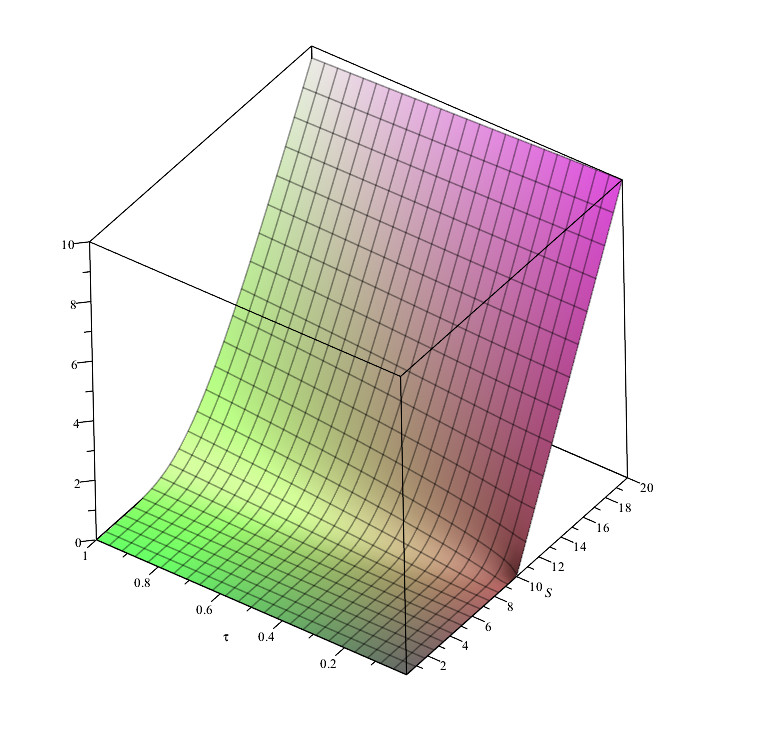
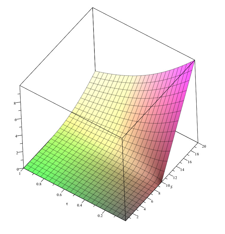
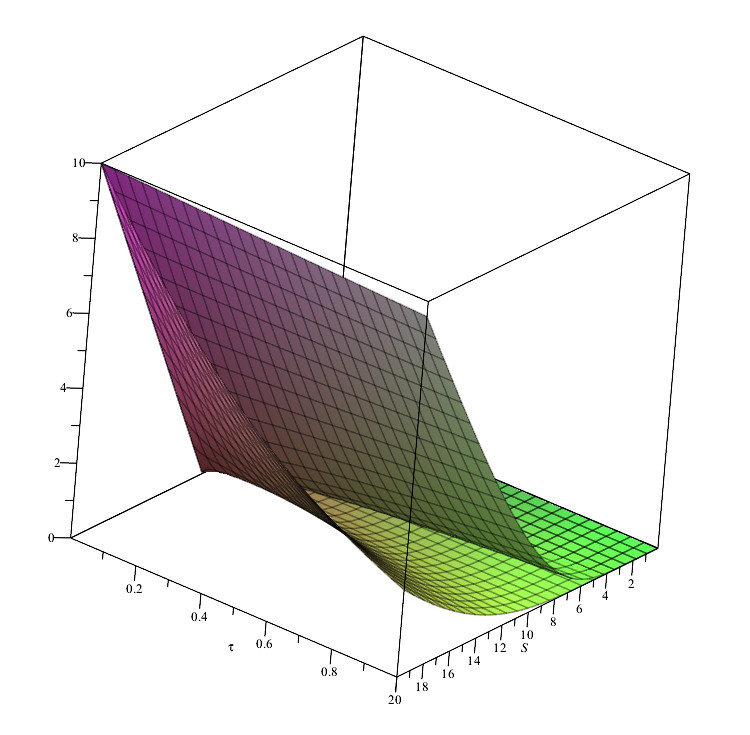
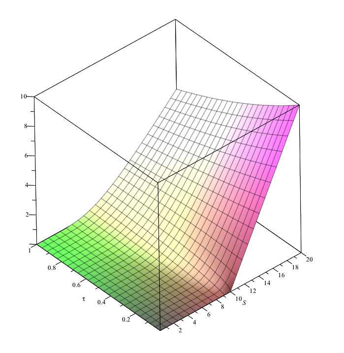
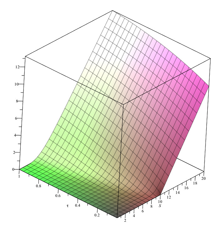
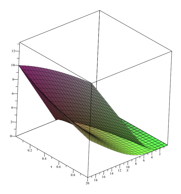
Figures (1) and (1) show the behavior of the weak and strong solution VV for two different parameter sets.
Refer to caption
Refer to caption
Refer to caption
Figure 1: From left to right: weak solution, strong solution and both solutions for E=10E=10, μ=0.8\mu=0.8, r=0.2r=0.2, σ=0.4\sigma=0.4 in the pure Call case.

Refer to caption
Refer to caption
Refer to caption
Figure 2: From left to right: weak solution, strong solution and both solutions for E=10E=10, μ=0.2\mu=0.2, r=0.8r=0.8, σ=0.4\sigma=0.4 in the pure Call case.

Finally, one must note that all of these results are valid if μ\mu, σ\sigma, μf\mu_{f} and Γ\Gamma are functions of the space–time variables (S,f,t)(S,f,t) that satisfy the asymptotic behavior

limf0μ(S,f,t)μ0limf0σ(S,f,t)σ0limf0μf(S,f,t)μf0limf0Γ(S,f,t)Γ0limfμ(S,f,t)μlimfσ(S,f,t)σlimfμf(S,f,t)μflimfΓ(S,f,t)Γ,\begin{aligned} \lim_{f\rightarrow 0}&\ \mu(S,f,t)\ &\approx&\ \ \mu^{0}\\ \lim_{f\rightarrow 0}&\ \sigma(S,f,t)\ &\approx&\ \ \sigma^{0}\\ \lim_{f\rightarrow 0}&\ \mu_{f}(S,f,t)\ &\approx&\ \ \mu_{f}^{0}\\ \lim_{f\rightarrow 0}&\ \Gamma(S,f,t)\ &\approx&\ \ \Gamma^{0}\end{aligned}\ \ \ \ \ \ \ \ \ \ \ \ \ \ \ \ \begin{aligned} \lim_{f\rightarrow\infty}&\ \mu(S,f,t)\ &\approx&\ \ \mu^{\infty}\\ \lim_{f\rightarrow\infty}&\ \sigma(S,f,t)\ &\approx&\ \ \sigma^{\infty}\\ \lim_{f\rightarrow\infty}&\ \mu_{f}(S,f,t)\ &\approx&\ \ \mu_{f}^{\infty}\\ \lim_{f\rightarrow\infty}&\ \Gamma(S,f,t)\ &\approx&\ \ \Gamma^{\infty},\end{aligned} (121)

for the Gaussian Bubble or

limf0μ(S,f,t)μ0limf0σ(S,f,t)σ0limf0μf(S,f,t)fμf0limf0Γ(S,f,t)fΓ0limfμ(S,f,t)μlimfσ(S,f,t)σlimfμf(S,f,t)fμflimfΓ(S,f,t)fΓ,\begin{aligned} \lim_{f\rightarrow 0}&\ \mu(S,f,t)\ &\approx&\ \ \mu^{0}\\ \lim_{f\rightarrow 0}&\ \sigma(S,f,t)\ &\approx&\ \ \sigma^{0}\\ \lim_{f\rightarrow 0}&\ \mu_{f}(S,f,t)\ &\approx&\ \ f\ \mu_{f}^{0}\\ \lim_{f\rightarrow 0}&\ \Gamma(S,f,t)\ &\approx&\ \ f\ \Gamma^{0}\end{aligned}\ \ \ \ \ \ \ \ \ \ \ \ \ \ \ \ \begin{aligned} \lim_{f\rightarrow\infty}&\ \mu(S,f,t)\ &\approx&\ \ \mu^{\infty}\\ \lim_{f\rightarrow\infty}&\ \sigma(S,f,t)\ &\approx&\ \ \sigma^{\infty}\\ \lim_{f\rightarrow\infty}&\ \mu_{f}(S,f,t)\ &\approx&\ \ f\ \mu_{f}^{\infty}\\ \lim_{f\rightarrow\infty}&\ \Gamma(S,f,t)\ &\approx&\ \ f\ \Gamma^{\infty},\end{aligned} (122)

for the log-normal bubble. Here, μ0\mu^{0}, σ0\sigma^{0}, μf0\mu_{f}^{0}, Γ0\Gamma^{0}, μ\mu^{\infty}, σ\sigma^{\infty}, μf\mu_{f}^{\infty} and Γ\Gamma^{\infty} are constant.

6 Conclusions

In this article, a stochastic model of endogenous arbitrage bubbles was developed. In this case, the arbitrage bubble satisfies a stochastic differential equation (10), and the option price is given by the general equation (22). This equation has several interesting limit behaviors. For example, for Γ=0\Gamma=0 in (22), there exist both “weak” f0f\approx 0 and “strong” ff\rightarrow\infty bubble regimens. The weak case corresponds to the usual arbitrage-free Black–Scholes model, while the strong case also corresponds to a Black–Scholes model where the interest rate has been changed by the mean value of the underlying assets.

For the case Γ0\Gamma\neq 0, it has been shown that similar weak and strong bubble behaviors exist for two different stochastic bubbles: the Gaussian and the lognormal bubbles. For a pure Call contract case, the dynamic equations of these weak and stronger limits are given by equations (42), (49) and (68) and (71), respectively. The solutions of these asymptotic equations are given by equations (94) and (104), which are equivalents to the Black–Scholes solution but with Γ0\Gamma\neq 0.
It is interesting to note that for the Gaussian bubble case, where ff can take positive and negative values, there exist another weak limit f/σ1f/\sigma\approx-1, whose dynamics are given by (54) with a solution given by (106). However, for the lognormal case, that limit cannot be reached because ff would always maintain positive according to (64).

Thus, the usual Black–Scholes theory can be considered as only an asymptotic limit of a more general model given by equation (22). Although the solutions studied here are limit cases of the general model (22), they are by no means important. Furthermore, these solutions can test the accuracy of the general case’s numerical solution in the different asymptotic scenarios.

In a forthcoming article, I will obtain the corresponding numerical solutions of (22) and compare them with the weak and strong limits solutions obtained in this paper.

References

  • [1] Black F and Scholes M 1973 The pricing of options and corporate liabilities J. Polit. Econ. 8 31 637–654
  • [2] Merton R 1973 Theory of rational option pricing Bell J. Econ. Manage. Sci. 4 1 141–183
  • [3] Heston S 1993 A close form solution for option with stochastic volatility, with applications to bond and currency options Rev. Financ. Stud. 6 327–343
  • [4] Hull J and White A 1987 The pricing of options on assets with stochastic volatilities The Journal of Finance 42 2 281–300
  • [5] Chen L 1996 Financial Markets, Institutions, and Instruments 5 1–88
  • [6] Baaquie B 1997 A Path Integral Approach to Option Pricing with Stochastic Volatility: Some Exact Results J. Phys. I France 7 12 1733–1753
  • [7] Gatheral J 2006 The Volatility Surface (Wiley)
  • [8] Cont R and Tankov P 2004 Financial Modelling with Jump Processes (Chapman and Hall/CRC)
  • [9] Wilmott P 2000 Paul Wilmott on Quantitative Finance (Wiley)
  • [10] T. Björk 2009 Arbitrage Theory in Continuous Time (Oxford University Press)
  • [11] Otto M 2000 Stochastic relaxational dynamics applied to finance: towards non-equilibriumoption pricing theory International Journal of Theoretical and Applied Finance 3 3 565
  • [12] Panayides S 2006 Arbitrage opportunities and their implications to derivative hedging Physica A 361 1 289–296
  • [13] Fedotov S and Panayides S 2005 Stochastic arbitrage return and its implication for option pricing, Physica A 345 1 207–217
  • [14] K. Ilinski 2001 Physics of Finance: Gauge Modelling in Non-equilibrium pricing (Wiley)
  • [15] Ilinski K 1999 How to account for the virtual arbitrage in the standard derivative pricing preprint.cond-mat/9902047
  • [16] Ilinski K and Stepanenko A 1999 Derivative Pricing with Virtual Arbitrage preprint.cond-mat/9902046
  • [17] Contreras M, Montalva R, Pellicer R and Villena M 2010 Dynamic option pricing with endogenous stochastic arbitrage Physica A 389 17 3552–3564
  • [18] Contreras M, Pellicer R, Ruiz A and Villena M 2010 A quantum model of option pricing: When Black–Scholes meets Schrödinger and its semi–classical limit Physica A 389 23 5447–5459
  • [19] Contreras M, Pellicer R, Santiagos D and Villena M 2016 Calibration and simulation of arbitrage effects in a non–equilibrium quantum Black–Scholes model by using semi–classical methods J. Math. Finance 6 541–561
  • [20] Contreras M, Echeverría J, Peña J and Villena M, 2020 Physica A 540 123238