Energetic instability of passive states in thermodynamics
Abstract
Passivity is a fundamental concept in thermodynamics that demands a quantum system’s energy cannot be lowered by any reversible, unitary process acting on the system. In the limit of many such systems, passivity leads in turn to the concept of complete passivity, thermal states, and the emergence of a thermodynamic temperature. In contrast, here we need only consider a single system and show that every passive state except the thermal state is unstable under a weaker form of reversibility. More precisely, we show that given a single copy of any athermal quantum state we may extract a maximal amount of energy from the state when we can use a machine that operates in a reversible cycle and whose state is left unchanged. This means that for individual systems the only form of passivity that is stable under general reversible processes is complete passivity, and thus provides a single-shot and more physically motivated identification of thermal states and the emergence of temperature. The machine which extracts work from passive states exploits the fact that one can find a subspace which acts as a virtual hot reservoir, and a subspace which acts as a virtual cold reservoir. We show that an optimal amount of work can be extracted, and that the machine operates at the Carnot efficiency between pairs of virtual reservoirs.
I Introduction
Within thermodynamics, heat engines are devices that operate in a thermal context so as to extract ordered energy in the form of work. The canonical scenario involves an engine that operates cyclically between two temperatures , and performs a quantity of mechanical work. To do so the engine absorbs heat from the hot reservoir, converts some of this energy to mechanical work and releases heat into the cold reservoir in accordance with the Second Law of thermodynamics. The largest possible efficiency, , occurs for the reversible Carnot engine carnot_reflections_1824 ; callen_thermodynamics_1985 and provides a fundamental thermodynamic bound on the amount of ordered energy that can be obtained. Carnot engines, and more in general heat engines, have been extensively studied in the microscopic regime scully_extracting_2003 ; scovil_three-level_1959 ; geusic_quantum_1967 ; alicki_quantum_1979 ; howard_molecular_1997 ; geva_classical_1992 ; hanggi_artificial_2009 ; feldmann_quantum_2006 ; rousselet_directional_1994 ; faucheux_optical_1995 ; linden_how_2010 ; horodecki_fundamental_2013 ; brunner_virtual_2012 ; tajima_optimal_2014 ; ito_optimal_2016 ; verley_unlikely_2014 ; gardas_thermodynamic_2015 ; uzdin_collective_2015 ; uzdin_quantum_2016 ; kosloff_quantum_2016 ; woods_maximum_2015 ; frenzel_quasi-autonomous_2016 ; lekscha_quantum_2016 ; niedenzu_operation_2016 (as well as, of course, in the macroscopic regime).
However, the issue of ordered energy extraction can also be considered in scenarios in which no notion of temperature exists, and can provide a broader notion of equilibrium states. For example, more general equilbrium states can occur in physical realisations when a system has been perturbed and has not had enough time to fully thermalise. They can also arise in the context of non-equilibrium steady states seifert2012stochastic . Given a quantum system in a state one can ask if it is possible to extract energy from it solely by performing a reversible unitary transformation on the system. The largest amount of ordered energy that can be extracted (the “ergotropy”, see Refs. allahverdyan_maximal_2004 ; alicki_entanglement_2013 ; sparaciari_resource_2016 ) depends non-trivially on the quantum state. If no energy can be extracted in this way then is called passive pusz_passive_1978 ; lenard_thermodynamical_1978 ; perarnau-llobet_extractable_2015 ; perarnau-llobet_most_2015 ; hovhannisyan_entanglement_2013 and constitutes a primitive form of equilibrium.
In this work, we consider a scenario that is intermediate between the above two contexts, and is motivated by the fact that a work extraction machine should be considered as a system which is involved in the process. Our core question is whether there exist passive states for which energy can be extracted if one performs a reversible unitary process over the system together with a second quantum system , which starts and finishes in the same quantum state . This second quantum system is the machine, such as the working body in a Carnot cycle, which undergoes a cyclic evolution. This class of processes is reminiscent of the ones taking place inside heat engines, and has been termed a catalytic thermal operation brandao_second_2013 .
Indeed, the system described by a passive state represents both the reservoirs, while the additional system is the machine which exchanges energy with the reservoirs in a cyclic manner. Due to the fact that microscopic heat engines can nowadays be realised in the laboratory scovil_three-level_1959 ; rousselet_directional_1994 ; faucheux_optical_1995 ; howard_molecular_1997 ; schulman_molecular_1999 ; scully_quantum_2002 , it seems reasonable to extend the analysis on passive states to the case in which this broader class of operations is allowed. Crucially, this analysis has fundamental implications for the notion of passivity. In fact, if energy can be extracted from a passive state with these reversible processes, and no entropy is generated, then it seems that associating passivity of the state is a restricted idealisation, unstable under this simple extension.
The paper is structured as follows. In Sec. II we provide the definition of passive and completely passive states, together with their description in terms of virtual temperatures. Any three levels of a passive state can be thought of as containing a subsystem which acts as a virtual hot reservoir, and one which acts as a virtual cold one. Sec. III provides the description of a protocol involving finite-sized engines which enable us to extract work in a cyclic way from a single passive state. In Sec. IV we prove that in fact any passive state which is not thermal can be activated by such an engine. Finally in Sec. V we show that such an activation can be done optimally via a quasi-static, reversible process with zero generation of entropy. We provide a simple expression for the amount of work which can be extracted from an arbitrary passive state, Eq. (38), and show that our machine can operate at the efficiency of a Carnot engine operating between two virtual heat reservours. We conclude that the only states in the single-shot regime that are stable under general reversible processes are thermal states.
II Passive states
Consider a finite-dimensional quantum system associated with the Hilbert space (a qudit), with Hamiltonian , and described by the state . We say that the state is passive iff its average energy cannot be lowered by acting on it with unitary operations, that is,
| (1) |
This implies that no work can be extracted from the state via a unitary process, since by conservation of energy, lowering the energy of a system would mean that this energy has been transfered to a work storage device.
We can also introduce a more restrictive notion of passivity. Let us consider independent and identically distributed (i.i.d.) copies of our system, with a total Hamiltonian , where each is a single-system Hamiltonian acting on a different copy of the system. The state of this global system is described by . Then, we say that the state is completely passive if and only if the state is passive for all . It can be shown pusz_passive_1978 that the completely passive states of a system with Hamiltonian are the ones satisfying the KMS condition kubo_statistical-mechanical_1957 ; martin_theory_1959 ; haag_equilibrium_1967 . Specifically, these states are the ground state and the thermal states with temperature , that is, with . Any state which is not of this form, is called athermal.
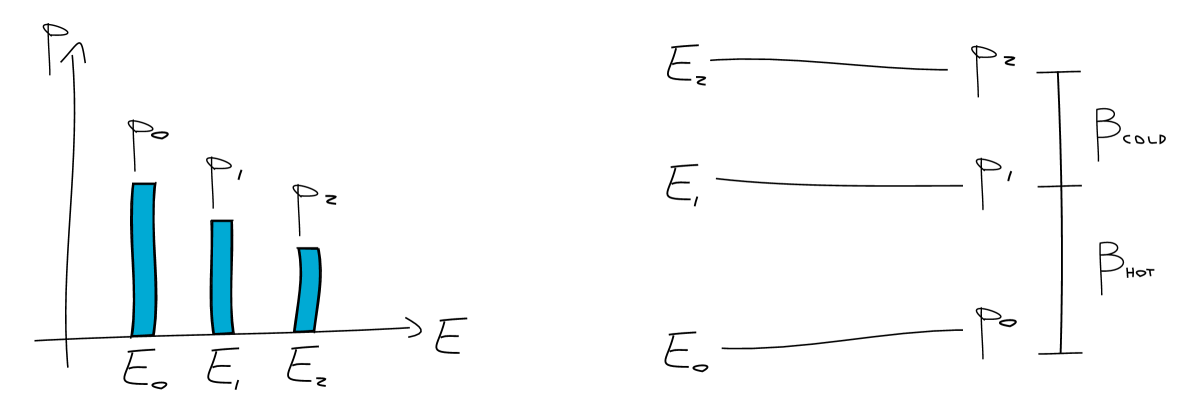
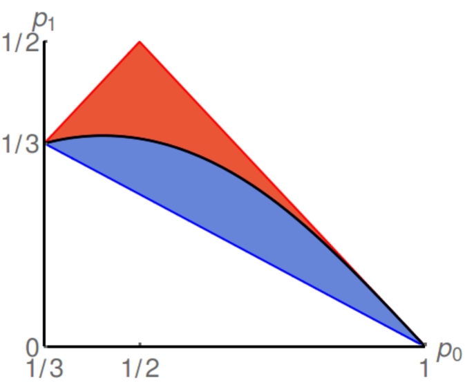
A characterization of all passive states can be easily obtained. A system in a passive state is such that the ground state has the highest probability of being occupied, and the probability of occupation decreases as the energy associated with the eigenstate of increases, Fig. 1, left plot. Specifically, a state is passive iff , where is a monotone non-increasing function. Simply put, this means that the state can expressed as
| (2) |
where are the eigenvectors of , ordered so that for all (for the case of equal energies we must make an additional stability assumption to ensure that ).
We can describe the probability distribution of the passive state by using virtual temperatures brunner_virtual_2012 ; skrzypczyk_passivity_2015 . In fact, for any given passive state, we can associate a (non-negative) virtual temperature with each pair of its eigenstates. For example, if we consider the pair , we define the virtual temperature associated with them as the such that
| (3) |
where is the probability of occupation of the state , and is the energy associated with the state (similarly for ). Thus, each pair of states can be regarded as an effective thermal state at a specific temperature. When all pairs of states has the same virtual temperature, we have that the passive state is completely passive, that is, it is the thermal state of at that temperature.
III The core protocol
We now introduce an engine that extracts work by acting individually on a passive state. The engine is composed by two main elements, namely, a qudit “machine” system with trivial Hamiltonian (), and a particular passive state. It suffices to consider qutrit systems, as a similar construction works more generally. The qutrit is assumed to have a Hamiltonian
| (4) |
and . The qutrit system is described by the state
| (5) |
where (Fig. 1, left plot).
In the following we assume that the passive state is described by the virtual temperature associated with the pair of eigenstates , and the virtual temperature associated with the pair . We assume for simplicity that , but a similar analysis applies for . In the Supplemental Material, Sec. I, the cycle is presented in full detail. The relation between the probability distribution of and the temperatures and is given by
| (6a) | ||||
| (6b) | ||||
where , and . Thus, the pair of states can be viewed as representing a “hot virtual reservoir”, while the pair of states represent a “cold virtual reservoir”. It is worth noting that the other pair of states, , is associated with a virtual temperature that is intermediate between and , as we can easily verify from Eqs. (6).
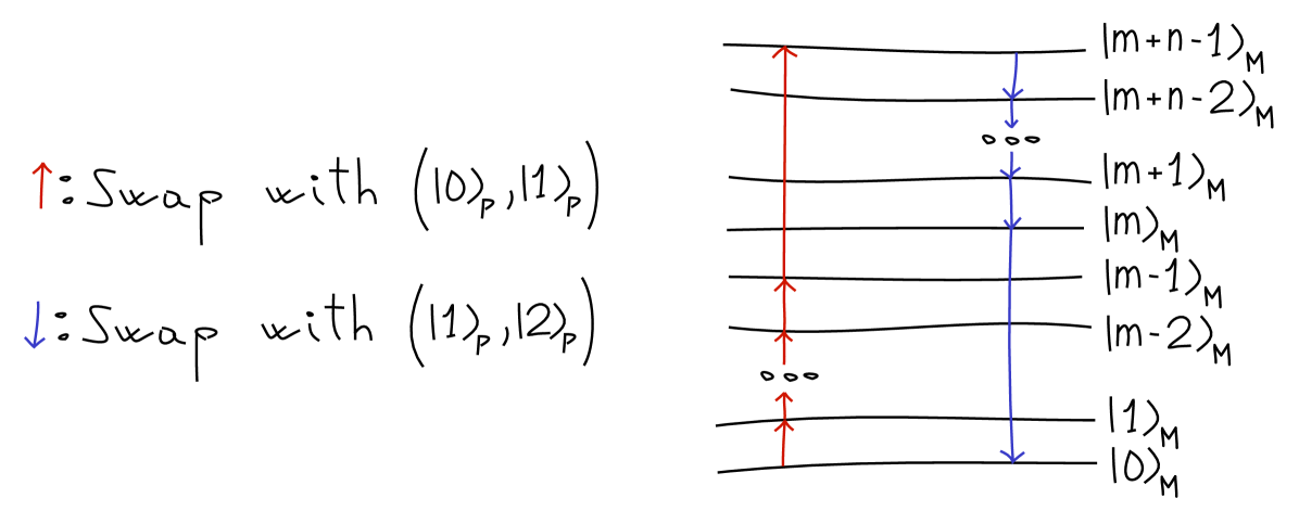
The engine extracts work by means of the following cycle. A single system, described by the state , is put in contact with the machine, described by the state . Then, we perform swaps between the hot virtual reservoir of the passive state and different pairs of states of , followed by swaps between the cold virtual reservoir and other different pairs of states of . In order to perform the swaps on different pairs of states, we need the machine to have at least levels, and therefore we fix . Specifically, we apply the following unitary operation to the global system
| (7) |
where the operator is a swap between system and machine, performed through the permutation . A graphical representation of this global operation is shown in Fig. 2, where each swap is depicted by an arrow acting over the states of the machine. Although in the figure we represent the eigenstates of in a ladder, they are all associated with the same energy, and therefore the order in which we present them is only functional for visualising the cycle .
In order for the engine to be re-usable, we need the local state of the machine to end up in its initial state. Therefore, we impose the following constraint on the state of the machine,
| (8) |
Through Eq. (8) we can express the probability distribution of the machine in terms of the passive state (see the Supplemental Material for further details). In our model we do not explicitly include an additional system (a battery) for storing the energy we extract from the passive state. Instead, we implicitly assume the existence of this work-storage system, and we define the work extracted, , as the difference in average energy between the initial and final state of the main system (as the machine has a trivial Hamiltonian, and no interaction terms are present between system and machine). Thus, we have that
| (9) |
where the final state of the system is
| (10) |
It is worth noting that the final state of system and machine will in general develop correlations. These correlations are classical, and without them work would not be extracted during the cycle. However, they do not compromise the re-usability of the machine if applied to another uncorrelated quantum system.
For a given system Hamiltonian and a given cycle we can investigate the amount of work we extract from the state . In the Supplemental Material we provide all the necessary steps to evaluate in terms of the probability distribution of . We can express this quantity as
| (11) |
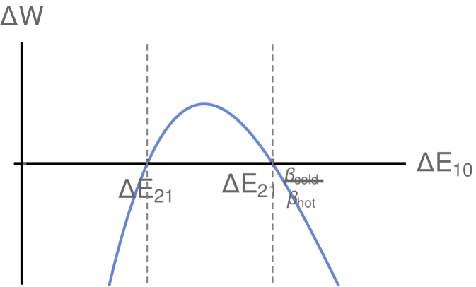
where is a positive coefficient depending non-trivially on the probability distribution of . For the class of passive states we are considering (namely, the one in which ), we find that work can be extracted () iff
-
1.
The Hamiltonian is such that .
-
2.
The temperatures of the two virtual reservoirs are such that .
Thus, for a fixed cycle (defined by the parameters and ), and for a fixed Hamiltonian , we find that work can only be extracted if the virtual temperature is lower than by a multiplicative factor which depends on the energy gaps of the Hamiltonian, see Fig. 3, left plot, for an example. In Sec. IV we show that, for a given Hamiltonian , work can be extracted by any passive (but not completely passive) state, and we characterise the cycle which allows for this extraction.
If we analyse in a more detailed way the cycle, we find that the same amount of energy is gained during each swap between the machine and the hot virtual reservoir, that is
| (12) |
where is the same positive coefficient of Eq. (11). Moreover, the same amount of energy is spent during each swap between the machine and the cold virtual reservoir,
| (13) |
Knowing the amount of energy exchanged during each swap allows us to evaluate the heat exchanged with the virtual reservoirs. In fact, if we identify the pair of levels with the hot virtual reservoir, then the energy exchanged during a swap with these levels can be considered as heat coming from the hot virtual reservoir. In this way, the total heat absorbed by the machine is
| (14) |
while the total heat provided to the cold virtual reservoir is
| (15) |
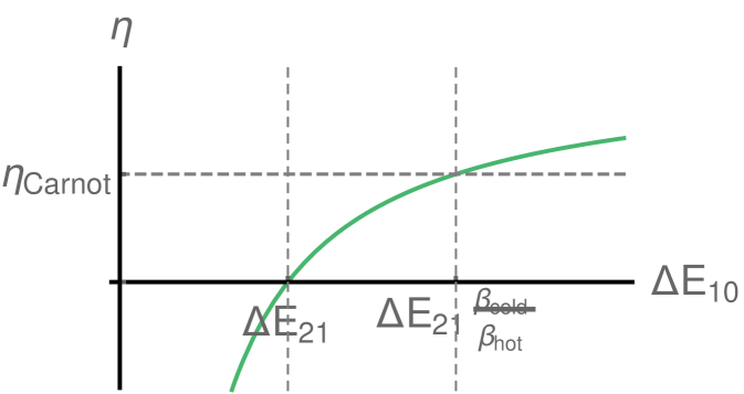
From Eqs. (14) and (15) we obtain that the work extracted can be expressed as , as in a standard heat engine exchanging energy between two reservoirs. Once and are defined, we can evaluate an efficiency of this cycle, that is
| (16) |
The efficiency of the engine (when the machine is finite-dimensional) is sub-Carnot in the virtual temperatures, see Fig. 3, right plot. In fact, work can only be extracted when conditions 1 and 2 are satisfied, and these conditions implied . When we consider the case of an infinite-dimensional machine, we find that by a judicious choice of parameters we may obtain Carnot efficiency.
Once the cycle is ended, the local state of the main system is moved to a less energetic state. By solving Eq. (8), we find that the final state of the main system has the following probability distribution
| (17a) | ||||
| (17b) | ||||
| (17c) | ||||
where the unit of probability depends on the initial state , and it is given by
| (18) |
with the same positive coefficient of Eq. (11). Due to condition 2, the unit , so that the probability of occupation of is reduced in favour of the probabilities and . Thus, energy is extracted from the passive state when is moved from to (during the hot swaps), and part of this energy is used to move the probability from to (during the cold swaps).
IV Work extraction from any passive state
We now show that, for a given Hamiltonian , work can be extracted from any passive but not completely passive state. In particular, we first show this for qutrit passive states, and we then generalise to the qudit case. Work extraction is achieved with the cycle presented in Sec. III, for specific values of the parameters and . In what follows, we represent the passive state with the probabilities of occupation , as opposed to the previous case in which the virtual temperatures were used. In this way, we can consider all possible scenarios, and we are not limited to the case in which a specific pair of eigenstates has a colder (hotter) virtual temperature than the other pair.
The Hamiltonian of the system is defined in Eq. (4), where the energy gap between ground and first excited state is , and the gap between first and second excited states is . We assume that
| (19) |
that is, we ask the ratio between the two energy gaps to be rational. Notice that, even if the ratio is irrational, we can find a suitable and such that the condition is approximatively satisfied. Once the relation between energy gaps is defined, we can divide the set of passive states into three different subsets, namely
| (20a) | ||||
| (20b) | ||||
| (20c) | ||||
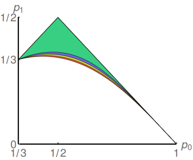
The union of these three subsets gives the set of all passive states. In particular, one can verify that the subset contains all the completely passive states, that is, the thermal states of at any temperature . Moreover, corresponds to the set of passive states with associated with the pair of eigenstates and , and associated with the pair and . The set , instead, contains the passive states with opposite hot and cold virtual temperatures. Since we are considering qutrit systems, we can represent the set of passive states in a two-dimensional diagram, using their probability distribution. Each point in this diagram represents a passive state. In Fig. 4, left plot, we show the three subsets of Eqs. (20).
In the previous section, we have seen that a cycle defined by the parameters and can activate a passive state with Hamiltonian if conditions 1 and 2 are satisfied. These conditions apply to the case in which the passive state is described by Eqs. 6, with . In the present, more general scenario we find that work is extracted by the cycle if and only if the passive state belongs to the following subset
| (21) |
where these conditions can be obtained by analysing the general expression of the extracted work, see Supplemental Material. We now show that, by tailoring the value of the parameters and , we can make to (asymptotically) cover either the region or . Here, we focus on solely, since follows from similar arguments. As a first step, we ask , which implies , due to Eq. (19). Then, in order to satisfy this condition, we set , where we ask to be large enough for to be an integer. The set of passive states activated by the cycle is such that
| (22) |
We notice that, since is passive, , which implies that
| (23) |
Thus, Eq. (22) and (23) together assure that . Moreover, if , we have that , which implies that . Thus, we have that, for a given Hamiltonian , and a given passive state , there exist a cycle such that . However, the closer (in trace norm) the state is to the set of completely passive states (), the larger the parameters and have to be, that is, the larger the machine has to be (see Fig. 4, right plot).
IV.1 Work extraction from a generic qudit passive state
Work extraction from a generic qudit passive state (for any Hamiltonian ) can be achieved with the cycle introduced in Sec. III, even if this work extraction is not optimal (as it might be when we deal with qutrit state, as we see in Sec. V). Indeed, even if the system has levels, we only need to focus our analysis on three of them, and perform the cycle on these levels only. Thus, given the state and the Hamiltonian , we can consider the subspace , for a given . Thus, we can divide the qudit state and the Hamiltonian in two contributions, one with support over , the other with support over its complement,
| (24a) | ||||
| (24b) | ||||
where the normalised quantum states are
| (25a) | ||||
| (25b) | ||||
while the Hamiltonian contributions are, respectively, and . In the following, we define , so that .
We can now introduce an ancillary system (the machine ) of dimension , described by the state , together with the global unitary operator ,
| (26) |
where the operator , described in Eq. (7), has support on , and therefore commute with . If we consider the evolution of the system under this operator, we obtain
| (27) |
and we can easily verify, due to the properties of , that the local state of the machine is left unchanged. The amount of work extracted during this cycle is
| (28) |
and the problem reduces to the one analysed at the beginning of this section (that is, to the extraction of work from a qutrit system described by the passive state , with Hamiltonian ), with the only difference of a multiplicative factor in .
IV.2 Work extraction and -activable states
The set of passive states can be divided into a hierarchy of classes, which divides the states according to the number of copies needed to activate them. Here, we say that a state is active if it is not passive, and therefore if we can extract work from it with unitary operations. Any passive but not completely passive state can be activated if we tensor together enough copies of it. In particular, when copies of a passive state are active, we call the state -activable. We now show that, if work is extracted from a qutrit passive state , with Hamiltonian , through the cycle , then the state realised by copies of is active. It worth noting that, while our cycle only requires an additional system of dimension to extract work from , in order to activate the same state we would need copies of it, that is, an ancilla whose size is exponential in .
In the following, we consider a qutrit system, although the same argument applies to qudit systems, for the reasons presented in the previous section. If the passive state is activated by the cycle , then one of the two conditions in Eq. (IV) has to be satisfied. Let us assume that the conditions satisfied by state and Hamiltonian are
| (29a) | ||||
| (29b) | ||||
where the other case follows straightforwardly.
Consider now a system composed by copies of the qutrit system under examination, with Hamiltonian , where the term acts over the -th copy. The state of this global system is . Then, let us focus our attention on two eigenstates of , namely, and . The first eigenstate has an energy of , and its occupation probability is . The second eigenstate, instead, has energy , and its occupation probability is . It is easy to verify that, if the constraints of Eqs. (29) hold, then the inequalities and are satisfied, implying that the state is active. Thus, we have shown that if a passive state can be activated with the cycle , then the state is active. However, this result does not tell us whether it is possible to activate the state by tensoring it with less copies. In the same way, we do not know whether the fact that the state is active implies that we can extract work from with the cycle .
V General Instability of Passive States
We can now establish our central claim: that any athermal passive state is energetically unstable under a reversible process that does not generate entropy. We analyse the evolution of a passive state which sequentially interacts with an infinite-dimensional machine , and find that the system moves through a continuous trajectory of passive states towards the set of minimum-energy states, that is, the set of the states jaynes_information_1957 .
We consider a cycle composed of infinitely many hot swaps, , and infinite many cold swaps, , with the assumption that , where is a parameter taking values in a specific range we will describe shortly. Let us now consider the situation in which the main system is a qutrit with Hamiltonian given in Eq. (4), described by the passive state whose probability distribution satisfies the equalities of Eqs. (6). Then, belongs to the subset defined in Eq. (20a), and the cycle has to satisfy conditions 1 and 2 in order to extract work from it. These conditions are reflected in the allowed range of the parameter , that is
| (30) |
If we set equal to a value inside the range specified by the previous equation, and we send , we find that (see Supplemental Material for details) the state of the machine as obtained from Eq. (8) is given by a mixture of two “thermal” states, one with effective temperature , the other with effective temperature (note we still have for the machine). These distributions have support in two different subspaces, and their weight depends non-trivially on the energy gaps of and on the virtual temperatures of . In fact, we can loosely interpret the state of the machine in terms of a thermal mixture
| (31) |
where
| (32) |
and
| (33) |
Notice that in order to define these “thermal states” we have introduced two fictitious Hamiltonians, namely, and . These operators are necessary if we want to consider the distribution of the machine as the mixture of two thermal distributions, but they do not enter in any way in the derivation of the extractable work. Indeed, as we have specified at the beginning of Sec. III, the machine can have any Hamiltonian (it does not modify the amount of work we extract during the cycle), and we choose to use a trivial one , so that the machine acts as a memory. The weight in the mixture is given by
| (34) |
Thus, during the cycle, the passive state first interacts with the “hot reservoir”, by performing a sequence of swaps between the pair of states and and the levels of . Then, the state interacts with the “cold reservoir”, performing a sequence of swaps between the pair and and the levels of .
In this scenario, we find that the probability distribution of the passive state is infinitesimally modified, and consequently the work extracted is infinitesimally small. In particular, we find that the unit of probability, defined in Eq. (18), tends to with an exponential scaling, for . Let us consider the probability distribution of the final state of the system . Since the distribution only changes infinitesimally during the cycle, we can recast Eqs. (17) as a set of differential equations (see the Supplemental Material for further details). Thus, we can imagine the situation in which infinite many machines are present, so that we can keep infinitesimally changing the state of the main system. In this case, the evolution of the state is governed by the following equation
| (35) |
where the parameter provides a continuum label for the sequence of cycles we perform on the passive state. We can then solve this equation for extremal cases for the function . When the parameter function is equal to one of its limiting values, Eq. (35) assumes a clear meaning. In fact,
-
•
when , then the differential equation can be recast as a condition over the average energy of the system, that is,
(36) Then, for taking this value, the passive state evolves along a trajectory that conserves the energy of the system.
-
•
when , instead, the differential equation can be recast as a condition over the entropy of the system, that is,
(37) where is the Von Neumann entropy. Then, for this , the passive state evolves along a trajectory that conserves the entropy of the system.
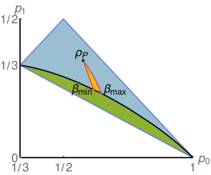
For taking values inside the allowed range, we have that any trajectory between the two presented above is possible, and the set of achievable states is shown in Fig. 5, left plot. It is possible to show that the evolution of the system moves the passive state toward the set of thermal states, which are the stationary states of this dynamic. In Fig. 5, right plot, we show the same set of achievable states, represented this time in the energy-entropy diagram sparaciari_resource_2016 . It is clear that, through this evolution, we can obtain any passive state with a smaller average energy and a bigger entropy than . In Supplemental Material, we show that these states are also the only ones that we can reach with our engines (and with a broader class of maps, called activation maps).
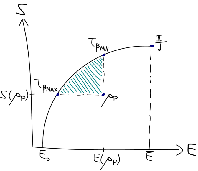
It is interesting to consider the limiting values of work extraction that can be achieved following the scheme suggested in this section. In particular, when the system evolves along the energy-preserving trajectory, the final state we obtain is the thermal state of at temperature , that is, , where the temperature is such that . In this case, it is easy to see that the engine is not extracting any work, and its only effect consists in raising the entropy of the system. If we consider the efficiency of this cycle, Eq. (16), we see that , as expected. The opposite limit is obtained when the system evolves along the entropy-preserving trajectory. In this case, the final state is , that is, the thermal state of at temperature , such that . In this case, the work extracted by the cycle is
| (38) |
that is the maximum amount one can extract alicki_entanglement_2013 ; sparaciari_resource_2016 . Significantly, in this case the efficiency is equal to the Carnot one, .
VI Conclusion
In the paper we have presented an engine that is able to extract work from any single copy of an athermal passive state. The engine utilises an ancillary system for the work extraction, and the local state of this system is recovered at the end of the cycle. In this way, the cycle can be run multiple times, and each time it acts on a new copy of the passive state. We show that, for any given Hamiltonian, work can be extracted from any passive, but not completely passive state. Moreover, we show that, in order to extract work from passive states close to the set of completely passive states, we need an ancillary system of large dimension. With an infinite dimension machine we can also evolve a passive state smoothly toward the set of thermal states. In particular, optimal work extraction can be obtained in this case, and it is achieved by mapping the initial state into the thermal state with the same entropy.
The present work provides some evidence that a resource theory for thermodynamics with an imperfect thermal reservoir presents non-trivial challenges. Such a resource theory could be realised by providing passive states for free. However, an obvious restriction we should make in this resource theory consists in the fact that we could not provide more than copies of a -activatable passive state, otherwise work might be extracted with unitary operations from this free state. Moreover, our results show that, even in the case in which a single passive state is provided, an ancillary system exists such that work can be extracted from the individual passive state. Then, in order to build a sensible resource theory, passive states should be always provided at a work cost, equal to the optimal amount of energy extractable from them when a machine is present.
It might also be interesting to analyse which passive states allow for the extraction of the highest amount of work in our cycle. In particular, this problem has been studied in the case of passive states and unitary evolution perarnau-llobet_most_2015 , and a comparison between that class of states and the class of states which allow for maximal work extraction during our cycle might be interesting.
Acknowledgements: We are grateful to Ben Schumacher and Michael Westmoreland for inspiring discussions. JO thanks the Royal Society and an EPSRC Established Career Fellowship for their support. CS is supported by the EPSRC [grant number EP/L015242/1]. DJ is supported by the Royal Society. We thank the COST Network MP1209 in Quantum Thermodynamics.
References
- (1) S. Carnot, Reflections on the Motive Power of Fire. 1824.
- (2) H. B. Callen, Thermodynamics and an Introduction to Thermostatistics. Wiley, 2nd ed., 1985.
- (3) M. O. Scully, M. S. Zubairy, G. S. Agarwal, and H. Walther, “Extracting Work from a Single Heat Bath via Vanishing Quantum Coherence,” Science, vol. 299, no. 5608, pp. 862–864, 2003.
- (4) H. E. D. Scovil and E. O. Schulz-DuBois, “Three-Level Masers as Heat Engines,” Physical Review Letters, vol. 2, no. 6, pp. 262–263, 1959.
- (5) J. E. Geusic, E. O. Schulz-DuBios, and H. E. D. Scovil, “Quantum Equivalent of the Carnot Cycle,” Physical Review, vol. 156, no. 2, pp. 343–351, 1967.
- (6) R. Alicki, “The quantum open system as a model of the heat engine,” Journal of Physics A: Mathematical and General, vol. 12, no. 5, p. L103, 1979.
- (7) J. Howard, “Molecular motors: structural adaptations to cellular functions,” Nature, vol. 389, no. 6651, pp. 561–567, 1997.
- (8) E. Geva and R. Kosloff, “On the classical limit of quantum thermodynamics in finite time,” The Journal of Chemical Physics, vol. 97, no. 6, pp. 4398–4412, 1992.
- (9) P. Hänggi and F. Marchesoni, “Artificial Brownian motors: Controlling transport on the nanoscale,” Reviews of Modern Physics, vol. 81, no. 1, pp. 387–442, 2009.
- (10) T. Feldmann and R. Kosloff, “Quantum lubrication: Suppression of friction in a first-principles four-stroke heat engine,” Physical Review E, vol. 73, no. 2, p. 025107, 2006.
- (11) J. Rousselet, L. Salome, A. Ajdari, and J. Prostt, “Directional motion of brownian particles induced by a periodic asymmetric potential,” Nature, vol. 370, no. 6489, pp. 446–447, 1994.
- (12) L. P. Faucheux, L. S. Bourdieu, P. D. Kaplan, and A. J. Libchaber, “Optical Thermal Ratchet,” Physical Review Letters, vol. 74, no. 9, pp. 1504–1507, 1995.
- (13) N. Linden, S. Popescu, and P. Skrzypczyk, “How Small Can Thermal Machines Be? The Smallest Possible Refrigerator,” Physical Review Letters, vol. 105, no. 13, p. 130401, 2010.
- (14) M. Horodecki and J. Oppenheim, “Fundamental limitations for quantum and nanoscale thermodynamics,” Nature Communications, vol. 4, 2013.
- (15) N. Brunner, N. Linden, S. Popescu, and P. Skrzypczyk, “Virtual qubits, virtual temperatures, and the foundations of thermodynamics,” Physical Review E, vol. 85, no. 5, p. 051117, 2012.
- (16) H. Tajima and M. Hayashi, “Optimal Efficiency of Heat Engines with Finite-Size Heat Baths,” arXiv:1405.6457 [cond-mat, physics:quant-ph], 2014.
- (17) K. Ito and M. Hayashi, “Optimal performance of generalized heat engines with finite-size baths of arbitrary multiple conserved quantities based on non-i.i.d. scaling,” arXiv:1612.04047 [quant-ph], 2016.
- (18) G. Verley, M. Esposito, T. Willaert, and C. Van den Broeck, “The unlikely Carnot efficiency,” Nature Communications, vol. 5, p. 4721, 2014.
- (19) B. Gardas and S. Deffner, “Thermodynamic universality of quantum Carnot engines,” Physical Review E, vol. 92, no. 4, 2015.
- (20) R. Uzdin, “Collective operation of quantum heat machines via coherence recycling, and coherence induced reversibility,” arXiv:1509.06289 [quant-ph], 2015.
- (21) R. Uzdin, A. Levy, and R. Kosloff, “Quantum heat machines equivalence and work extraction beyond Markovianity, and strong coupling via heat exchangers,” Entropy, vol. 18, no. 4, p. 124, 2016.
- (22) R. Kosloff and Y. Rezek, “The quantum harmonic Otto cycle,” arXiv:1612.03582 [quant-ph], 2016.
- (23) M. P. Woods, N. Ng, and S. Wehner, “The maximum efficiency of nano heat engines depends on more than temperature,” arXiv:1506.02322 [cond-mat, physics:quant-ph], 2015.
- (24) M. F. Frenzel, D. Jennings, and T. Rudolph, “Quasi-autonomous quantum thermal machines and quantum to classical energy flow,” New Journal of Physics, vol. 18, no. 2, p. 023037, 2016.
- (25) J. Lekscha, H. Wilming, J. Eisert, and R. Gallego, “Quantum thermodynamics with local control,” arXiv:1612.00029 [quant-ph], 2016.
- (26) W. Niedenzu, D. Gelbwaser-Klimovsky, A. G. Kofman, and G. Kurizki, “On the operation of machines powered by quantum non-thermal baths,” New Journal of Physics, vol. 18, no. 8, p. 083012, 2016.
- (27) U. Seifert, “Stochastic thermodynamics, fluctuation theorems and molecular machines,” Reports on Progress in Physics, vol. 75, no. 12, p. 126001, 2012.
- (28) A. E. Allahverdyan, R. Balian, and T. M. Nieuwenhuizen, “Maximal work extraction from finite quantum systems,” Europhysics Letters (EPL), vol. 67, no. 4, pp. 565–571, 2004.
- (29) R. Alicki and M. Fannes, “Entanglement boost for extractable work from ensembles of quantum batteries,” Physical Review E, vol. 87, no. 4, 2013.
- (30) C. Sparaciari, J. Oppenheim, and T. Fritz, “A Resource Theory for Work and Heat,” arXiv:1607.01302 [cond-mat, physics:quant-ph], 2016.
- (31) W. Pusz and S. L. Woronowicz, “Passive states and KMS states for general quantum systems,” Communications in Mathematical Physics, vol. 58, no. 3, pp. 273–290, 1978.
- (32) A. Lenard, “Thermodynamical proof of the Gibbs formula for elementary quantum systems,” Journal of Statistical Physics, vol. 19, no. 6, pp. 575–586, 1978.
- (33) M. Perarnau-Llobet, K. V. Hovhannisyan, M. Huber, P. Skrzypczyk, N. Brunner, and A. Acín, “Extractable Work from Correlations,” Physical Review X, vol. 5, no. 4, 2015.
- (34) M. Perarnau-Llobet, K. V. Hovhannisyan, M. Huber, P. Skrzypczyk, J. Tura, and A. Acín, “Most energetic passive states,” Phys. Rev. E, vol. 92, no. 4, p. 042147, 2015.
- (35) K. V. Hovhannisyan, M. Perarnau-Llobet, M. Huber, and A. Acín, “Entanglement Generation is Not Necessary for Optimal Work Extraction,” Physical Review Letters, vol. 111, no. 24, 2013.
- (36) F. G. S. L. Brandao, M. Horodecki, N. H. Y. Ng, J. Oppenheim, and S. Wehner, “The second laws of quantum thermodynamics,” Proc. Natl. Acad. Sci., vol. 112, no. 11, pp. 3275–3279, 2015.
- (37) L. J. Schulman and U. V. Vazirani, “Molecular Scale Heat Engines and Scalable Quantum Computation,” in Proceedings of the Thirty-first Annual ACM Symposium on Theory of Computing, STOC ’99, (New York, NY, USA), pp. 322–329, ACM, 1999.
- (38) M. O. Scully, “Quantum Afterburner: Improving the Efficiency of an Ideal Heat Engine,” Physical Review Letters, vol. 88, no. 5, p. 050602, 2002.
- (39) R. Kubo, “Statistical-Mechanical Theory of Irreversible Processes. I. General Theory and Simple Applications to Magnetic and Conduction Problems,” Journal of the Physical Society of Japan, vol. 12, no. 6, pp. 570–586, 1957.
- (40) P. C. Martin and J. Schwinger, “Theory of many-particle systems. I,” Physical Review, vol. 115, no. 6, p. 1342, 1959.
- (41) R. Haag, N. M. Hugenholtz, and M. Winnink, “On the equilibrium states in quantum statistical mechanics,” Communications in Mathematical Physics, vol. 5, no. 3, pp. 215–236, 1967.
- (42) P. Skrzypczyk, R. Silva, and N. Brunner, “Passivity, complete passivity, and virtual temperatures,” Phys. Rev. E, vol. 91, no. 5, p. 052133, 2015.
- (43) E. T. Jaynes, “Information theory and statistical mechanics,” Physical review, vol. 106, no. 4, p. 620, 1957.
Supplemental Material
Appendix A General cycle for work extraction from passive states
We present in full details the general cycle needed to extract work from a qutrit system described by a passive state. Work extraction is achieved through the interaction between a qudit ancilla (the thermal machine) and the main qutrit system. This qutrit system has Hamiltonian
| (39) |
and we define the energy gap as and . The state of the system is passive, meaning that no energy can be extracted with unitary operations, and we can write it as a classical state
| (40) |
where (which is a direct consequence of the no-energy-extraction condition).
The machine we introduce is a -level system with a trivial Hamiltonian, described by the state
| (41) |
We operate over system and machine with a unitary operation composed by multiple swaps. In particular, we first perform swaps between the pair of states and the pairs , followed by a swap between the same pair of states of the system and the pair of the machine. Then, we perform swaps between the pair and the pairs , followed by a swap between the same system’s states and the pair . In order to perform this cycle, the dimension of the catalyst has to be at least equal to , and indeed in the following we fix . The unitary we want to apply is
| (42) |
where the operation is a swap between system and machine, performing the permutation .
For the given unitary evolution we can easily evaluate the final state of the global system. This final state presents classical correlations between system and machine, but in the following we only consider the marginal states for system and machine, which are the sole information we need. In fact, the energy of the global system solely depends on the Hamiltonian of the system (and therefore only on the local state of the system), as the machine has a trivial Hamiltonian, and we do not have an interaction term . Moreover, in order for the machine to be re-usable on a new system, we only need its local initial and final states to be equal, and the correlations with the old systems do not affect the engine. The final state of the system is
| (43) |
while the final state of the machine is
| (44) |
As we stated above, in order for the machine to be re-usable we need its final local state to be equal to the initial one . Correlations with the system do not invalidate the re-usability, as we always discard the system after the cycle, and we take a new copy to repeat the process. In this way, we can extract work from a reservoir of passive states by acting on them individually. The constraint of an equal initial and final state of the machine provides the following set of equalities,
| (45a) | ||||
| (45b) | ||||
| (45c) | ||||
| (45d) | ||||
| (45e) | ||||
| (45f) | ||||
which, if solved, allow for the probability distribution of the state of the machine to be expressed in terms of the passive state .
A.1 Work extracted and activable passive states
In our framework, we do not explicitly account for a battery, that is, an additional system with a specific Hamiltonian, able to account for any energy exchange between system and machine. Instead, we implicitly assume the battery to be present, so that any change in the average energy of the system is thought as some energy flowing from (or to) the battery. In particular, if the average energy of the system decreases, then the battery is storing this energy, while when the average energy of the system increases, the battery is providing it. All the energy coming from (or going to) the battery is accounted as work. Under this assumptions, the amount of work we extract during one cycle is given by the changing in the average energy of the system, that is
| (46) |
where is the initial passive state, and is the final state, whose probability distribution is . We can express the amount of extracted work in terms of the energy gaps of the Hamiltonian , as
| (47) |
where this expression has been obtained by applying the normalisation constraint to the initial and final state of the system.
If we replace the probability distribution of the final state of the system, Eq. (A), into the expression of extracted work, Eq. (47), we obtain that
| (48) |
This expression can be highly simplified if we use the properties of the probability distribution of the machine, Eqs. (45). In particular, from Eq. (45b) we find that
| (49) |
while from (45c) we have that
| (50) |
Together, these equations reduce the first bracket of Eq. (48) into a single term,
| (51) |
If we consider Eq. (45e), instead, we find that
| (52) |
while Eq. (45d) implies that
| (53) |
These two equations simplify the second bracket of Eq. (48),
| (54) |
We can now use Eq. (45f) to show that
| (55) |
which allows us to express the work we extract as
| (56) |
From the above equation we notice that the work extracted is factorised into an Hamiltonian contribution and another contribution associated with the probability distribution of the passive state. Then, for a given Hamiltonian such that , we will find that certain passive states allow for work extraction (the ones in which ), while others do not. Therefore, for every given Hamiltonian (that is, every and ) and for every given cycle (that is, every and ), we find that the set of passive states is divided into two subsets, the ones which allow for work extraction (we can call them activable states), and the ones which do not. In the following we will express the probability distribution of in terms of the probability distribution of the passive state, so as to define these two subsets for each Hamiltonian and cycle.
As a first step, we want to express the first elements of the sequence in terms of last two elements, and . Moreover, we express the first elements of in terms of and . This can be done by utilising the equalities given in Eqs. (45b) and (45e), which we recast in the following way.
| (57a) | ||||
| (57b) | ||||
It can be proved (see the technical result 1) that the elements of the sequences can be expressed as
| (58a) | ||||
| (58b) | ||||
where and .
We can now express, using Eqs. (45c) and (45f), the elements and in terms of and . From Eq. (45c) we obtain that
| (59) |
From Eq. (45f), instead, we get that
| (60) |
Then, we can finally express in terms of through Eq. (45d), and we obtain
| (61) |
where the coefficient is defined as
| (62) |
Thanks to the above result, we can express the overall probability distribution of in terms of the occupation probability of the state . Thus, we have that
| (63a) | ||||
| (63b) | ||||
| (63c) | ||||
where it is possible to show that each , with , is positive if is positive (see the technical result 2). From the normalisation condition it then follows that the sequence is a proper probability distribution. Moreover, the normalisation condition allows us to evaluate as a function of the probability distribution of the passive state ,
| (64) |
From Eq. (64) we can express all the other elements of in terms of the probability distribution of .
We can now further characterise the amount of work extracted during our cycle. In fact, if we apply Eq. (63c) into Eq. (56), we obtain
| (65) |
where the sign of depends on the sole terms and , since the other factors are always positive. Thus, for each cycle, we can characterise which passive states can be activated by that cycle, that is, which states allow for work extraction during the cycle. The subset of activable states is
| (66) |
where this region clearly depends on the Hamiltonian of the system , and on the number of swaps performed during the cycle, and .
A.2 The final state of the system
Let us consider the final state of the passive system after we have applied the cycle . In Eq. (A) we have shown the probability distribution of as a function of . Thanks to the constraints introduced in Eqs. (45), we can simplify the form of , so that we obtain
| (67a) | ||||
| (67b) | ||||
| (67c) | ||||
We can easily notice that the cycle acts on the passive state by modifying the original probabilities by multiples of
| (68) |
The expression of the final state allows us to understand how the cycle operates over the system when work is extracted. In particular, we can consider the evolution of the system in two different situations, linked to the two possible scenarios of Eq. (A.1).
Suppose that is such that . Then, from the conditions in , we can verify that , so that the map is depleting the population of the state , while increasing the populations of both and (see Fig. 6, left plot). Work is extracted from the cycle since the energy gained while moving from to is bigger than the energy paid to move from to . In Sec. C, we show that the entropy of the system has to increase during the transformation. This is achieved since gets closer to after the cycle.
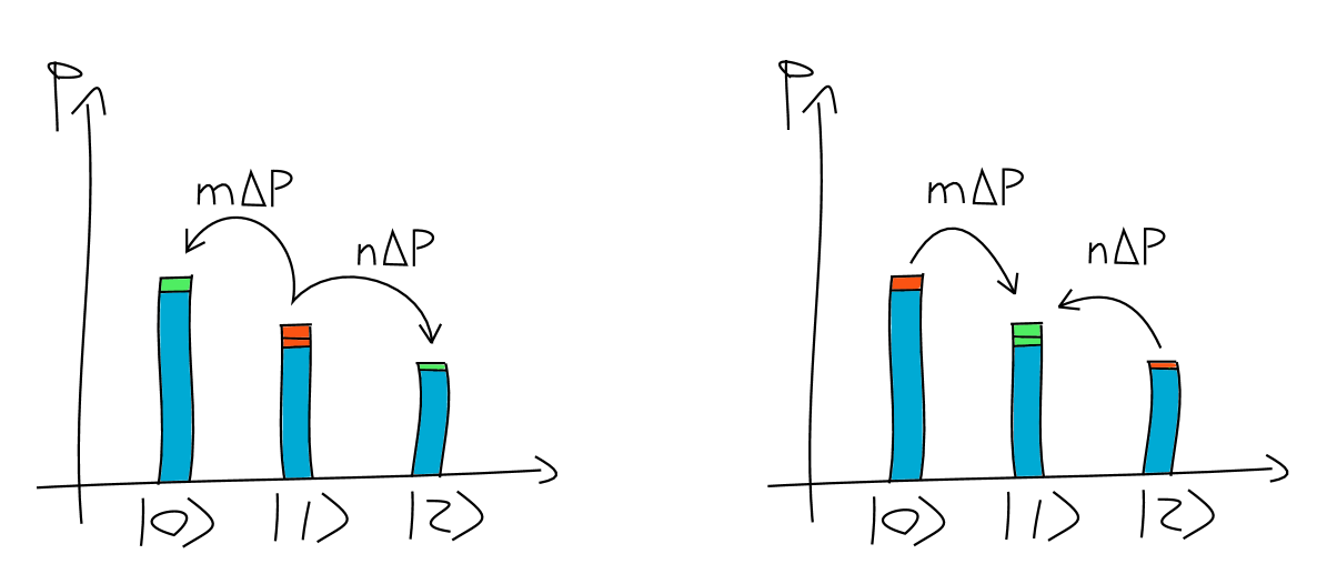
Let us consider the case in which is such that . Then, from the conditions in , we can verify that , so that the map is depleting the populations of the states and , while increasing the populations of (see Fig. 6, right plot). Work is extracted from the cycle since the energy gained while moving from to is bigger than the energy paid to move from to . Moreover, the entropy of the system increases since gets closer to after the cycle.
It is worth noting that the final state can be active. This happen, in the case of , when . In the other case, we obtain a final active state if . In these situations, not only are we able to extract work from the passive state during the cycle, but we can also perform a local unitary operation (permuting and in the first case, and and in the second) which allows for additional work extraction. It is also possible for the final state of the system to be passive, and to still lie inside the activable region . Due to the correlation created between system and machine, however, this state cannot be used again, at least not with the same machine.
Appendix B Asymptotic behaviour of the machine
We are now interested in the study of the cycle when the size of the machine (as well as the number of hot and cold swaps) tends to infinity. In particular, we are interested in the form of the probability distribution of the machine, the work extracted, and the final state of the passive system. Let us consider the Hamiltonian of the main (qutrit) system. We know that, for any Hamiltonian , there exists two integer numbers and such that . We now consider a passive state describing this system whose probability distribution satisfies . Notice that this condition implies that the state is in the subset of passive states denoted by (see the main text, Fig. 5), or equivalently it implies that the hot virtual temperature is associated with the pair of states and . One could analyse the opposite situation as well, but the results we obtain would be analogous, due to the symmetry of the problem with respect to the hot and cold interactions.
In order to perform the asymptotic expansion of the probability distribution of the machine, Eqs. (63), we first want to define how the ratio behaves as the number of hot and cold swaps goes to infinity. We set this fraction equal to , so that , and we define a range for this parameter, due to the constraints we set on the passive state. Indeed, if we want to extract work, we need and to satisfy one of the two conditions in Eq. (A.1), and in particular, since we assume the passive state to be in the region , we need and . The two inequalities implies that
| (69) |
where it is easy to verify that the lower bound is smaller than the upper one, due to the fact that .
We can now use the assumptions made on the cycle (that is, on the parameters and ) and on the initial passive state in order to expand the probability distribution of for . As a first step, let us consider the coefficient presented in Eq. (62). When and tends to infinity, we find that
| (70) |
where it is easy to verify that the term as , and that both and tends to 0 faster that this first term. However, we cannot say which one is the fastest without further assumptions, and that is the reason we keep both in the .
Once the expansion of is known, we can focus on the probability distribution of the machine. For simplicity, we consider the distribution in Eqs. (63), where is not defined yet; we will define it through the normalisation condition once the asymptotic expansion has been performed. We find that
| (71a) | ||||
| (71b) | ||||
| (71c) | ||||
We are now able to obtain the value of by imposing the normalisation condition over the asymptotic probability distribution of the machine. We find that
| (72) |
that is, tends to as for . Notice that the same result can be obtained by expanding Eq. (64). If we send and to infinity, we find that the asymptotic probability distribution of the machine is
| (73a) | ||||
| (73b) | ||||
| (73c) | ||||
We can now investigate how the probability distribution of the main system changes, and evaluate the asymptotic work extracted during on cycle. Let us consider the probability unit , introduced in Eq. (68). If we set and to infinity, we have that
| (74) |
that tends to 0 with an exponential scaling. Therefore, the heat engine with infinite-dimensional thermal machine only modifies the passive states by an infinitesimal amount. As a consequence, the work extracted has to be infinitesimal as well. Indeed, by considering Eq. (65) it is easy to show that tends to as , since is proportional to (modulo a multiplying factor proportional to , which tends to infinity more slowly than tends to ).
B.1 Final state and work extraction over multiple cycles
In the previous section we have seen that, when the machine is infinitely large, we only modify the passive state infinitesimally. We can then consider the situation in which we are given an infinite number of these machines, and we want to evolve the passive state (and extract work) by sequentially applying our cycle with the help of these machines. In order to study the evolution of the passive state, we can consider its probability distribution after one cycle, see Eqs. (67). These equations can be recast as differential equations, since in this scenario. It is easy to verify that the differential equations which govern the evolution of the passive state are
| (75a) | ||||
| (75b) | ||||
where takes values in the range given by Eq. (69), and we define
| (76) |
with the probability distribution of the state before the cycle, and the distribution of the state after the cycle. The continuous parameter is here related to the number of cycles we perform on the system. It is worth noting that Eqs. 75 share a common (positive) factor. Therefore we have that, as time goes on, the probability of occupation of increases, while the one of decreases (as expected from the discussion in Sec. A.2). Moreover, since , the increase in the former is slower than the decreasing of the latter.
The two differential equations can be reshaped in a single, more helpful one,
| (77) |
and we can investigate the solution of this equation for close to its limiting values. As a first step, let us consider the case in which . Then, the solution of Eq. (77) is
| (78) |
where is the probability distribution of the state of the system at time , and is the initial time (when the system is in ). If we rearrange Eq. (78), we see that it is equivalent to the following constraint for the evolved state
| (79) |
that is, the evolution conserves the energy of the system (equivalently, no work is extracted during the evolution). It is easy to see, for instance by representing the solution of Eq. (78) in a two-dimensional plot of versus , that the passive state is moving toward the set of thermal states, that are the steady states of this evolution. In fact, when a thermal state is considered, we find that , which implies . Thus, after enough time is passed, we find that the initial passive state has been mapped into the thermal state with inverse temperature , where
| (80) |
and is the partition function of the system at temperature .
We can now consider the case in which , that is, when its value is close to its lower bound. We notice that, in this case, itself depends on the probability distribution of the passive state. Then, if we replace with its lower bound in Eq. (77) we obtain
| (81) |
which, if integrated between time and time , gives the following constraint on the entropy of the evolved states
| (82) |
where is the Von Neumann entropy. Therefore, the evolution of the passive state has to preserve the entropy of the system, and the state is moving toward the set of thermal states. For , the system is in the thermal state with inverse temperature , where
| (83) |
and is the partition function of the system at temperature .
Thus, when we set equal to its limiting values, the evolution of the passive state can either follow a trajectory in which energy is conserved, or in which entropy is conserved. However, all intermediate trajectories can be achieved by imposing a different inside the range specified by Eq. (69), and consequently all passive states with lower or equal energy, and greater or equal entropy that can be reached.
Appendix C Activation maps
Consider a specific family of CPT maps which allow for work extraction from a system described by a passive state. The maps of this family, which we call activation maps, can be represented by unitary operations acting globally on both the main system and an ancilla, such that the local state of the ancillary system is preserved. The cycle of Sec. A is a particular instance of these activation maps, and in the following we study the main properties of this family. Let us consider a system with Hamiltonian , described by the state (this state does not need to be passive). The energy that we extract from the system when we evolve it with the unitary operator is given by the difference in average energy between the initial and final state,
| (84) |
We assume this energy to be stored in an implicit battery, and we refer to it as work. If the state is passive, then , that is, we cannot extract work. If the state is active, we can find some unitary operations that allow for a positive work extraction. In particular, the maximum work we can extract is
| (85) |
where the state is the passive state obtained from the initial state . In the literature, is known as ergotropy, see Ref. allahverdyan_maximal_2004 . This quantity is if the initial state is passive, and positive otherwise.
We now add an ancillary system with a trivial Hamiltonian, described by the state , and we consider the family of maps
| (86) |
where the unitary operator acts globally over system and ancilla, and we require that the final local state of the ancilla is equal to the initial one, that is,
| (87) |
Notice that the global evolution can create correlations between system and ancilla, and our sole constraint regards the local state of the ancilla. The work extracted during the evolution is given by
| (88) |
where the only contribution is given by the energy difference in the system, due to the absence of any interaction term between system and ancilla, and to the fact that the final state of the ancilla is equal to its initial one.
We can now introduce the notion of activation of a quantum state,
Definition 1.
Let us consider a system with Hamiltonian , described by the state . Then, we say that can be activated iff there exists an ancillary system with trivial Hamiltonian, described by the state , and an activation map as in Eq. (86), satisfying the condition of Eq. (87), such that
| (89) |
that is, if we can extract more work from by acting with than we can do by acting with any unitary operation.
As we noticed before, an example of activation map is the one used in our passive engine, Eq. (A), where the ancillary system is the machine, and the global unitary operation is .
C.1 General properties of the final state of an activation map
Although the family of maps introduced in the previous section is extremely general, we can still use their definition to derive some properties of the final state . The first, trivial property consists in the fact that the final state of an activation map has to have a lower energy than the one possessed by a the passified version of the initial state,
| (90) |
where this condition is obtained by replacing Eqs. (85) and (88) into Def. 1.
A second property regards the entropy of the final state. Due to the invariance of Von Neumann entropy under unitary operations, its sub-additivity, and the constraint on the local state of the machine, Eq. (87), we can show that
| (91) |
that is, the entropy of the system cannot decrease during the evolution through , and it increases if correlations create between system and machine.
If we use the two constraints on together, we can show that any completely passive state cannot be activated. In this case, in fact, we have that , that is, the state under examination is the thermal state of Hamiltonian for a certain . But we know that this state is the one with minimum energy for a given entropy, or, vice versa, the one with maximum entropy for given energy. Then, we cannot find another state such that the two conditions of Eqs. (90) and (91) are satisfied at the same time. This implies that any completely passive state cannot be activated, pure ground state and maximally-mixed state included.
We can also consider a generic pure state . The corresponding passified state is the ground state . From Eq. (90) it follows that the final state of has to have a lower energy than . But since the passified state we obtain, , is by definition the state with minimum energy, we cannot satisfy this condition. Thus, we cannot activate, in the sense of Def. 1, any pure state .
C.2 Asymptotic work extraction from passive states
It was proved by Alicki et al. (Ref. alicki_entanglement_2013 ) that, when an infinite number of copies of a passive state are considered, the optimal extractable work per single copy is given by
| (92) |
where is the thermal state with inverse temperature such that . We want to compare the work extracted in the asymptotic limit with the work extracted with a generic activation map . This comparison can be easily carried out using the main properties of the final state , see Eqs. (90) and (91), together with the properties of .
For any given final state of the system , there always exists an inverse temperature , and a thermal state at that temperature, such that . Since the state is thermal, we have that its energy is minimum, that is,
| (93) |
Moreover, from Eq. (91) it follows that the entropy of is greater than the entropy of the state , introduced in the previous paragraph. By considering this entropic condition together with the free energy difference , we obtain that the state is more energetic than , that is,
| (94) |
From the above inequalities we have that
| (95) |
Therefore, the energy we extract with the aid of an activation map is always equal or lower than the energy (per single copy) that we extract by acting over an infinite number of copies of the passive state with a global unitary operator, .
Thus, is an upper bound for the work extracted by any activation map . In Refs. alicki_entanglement_2013 ; sparaciari_resource_2016 it was shown that this upper bound can be actually achieved by acting over infinite many copies of the system with a global unitary operation. In this paper, instead, we have shown that the extraction of an amount of work equal to is also achievable by acting on a single copy of the state. However, one needs to utilise infinite many infinite-dimensional machines to do so, as we showed in Sec. B.
C.3 Ancilla as part of a bigger thermal bath
Consider the case in which the ancilla utilised in is just a subsystem of an infinite thermal reservoir at temperature . In this situation, we have to explicitly define an Hamiltonian (where we have the freedom to rigidly translate the spectrum of this Hamiltonian), so that the state of the ancilla coincides with the thermal state .
As we have seen, the map lowers the energy of the system and builds correlations between system and ancilla, while preserving the local state of the ancillary system. If we consider the ancilla as part of the infinite bath, then we see that extracts work from the passive state while no heat is exchanged with the bath (as the local state of the ancilla is unchanged). In the following we show that the energy extracted during this transformation is always lower than the difference in free energy between the initial state and the thermal state . Even in the case in which maps into , the work extracted is not optimal, as part of this work is locked inside the correlations between system and ancilla. In order to extract the remaining work from the correlations, and thus to perform optimal work extraction, we have to exploit the infinite thermal reservoir, exchanging an amount of heat proportional to the difference in entropy between and . It is worth noting that, although this second operation allows us to extract an higher amount of work than the one obtained with the sole , we do not consider it as an allowed operation in our framework, as it requires an additional ancillary system (the bath) with infinite dimension.
During the first operation we map the initial state into the final one . This final state might or might not be a thermal state of , and the sole constraints we have are given by Eqs. (90) and (91) (energy has to decrease while entropy has to increase). The work we extract is the energy difference between the initial and final state, as we show in Eq. (88),
| (96) |
which is positive by definition, since we assume to be an activation map, see Def. 1. The final state of system and ancilla is , and correlations are present, quantified by the mutual information
| (97) |
The heat exchanged during this transformation is equal to , as the local state of the bath does not change.
We now use the power of the infinite thermal reservoir to extract the last part of work from the state , by mapping it into . In this case, work is given by the free energy difference between the two states, that is
| (98) |
where is the relative entropy between and . Since both the relative entropy and the mutual information are non-negative quantities, we have that work is indeed extracted during this second process. The heat exchanged in this second transformation is equal to the entropy difference (modulo the multiplicative constant ) between the final and initial state
| (99) |
where the last equality follows from the invariance under unitary operations of the Von Neumann entropy.
If we now consider the two transformations as a single one, we see that the total work extracted is
| (100) |
that is, is optimal, and the heat exchanged is , equal to the entropy difference between and .
An interesting scenario occurs when maps the initial state into . In this case, we see that the work we obtain in the second transformation (the one involving the whole thermal bath) is proportional to the sole mutual information, so that work is exclusively extracted from the correlations between system and catalyst. The amount of work in this case (see also Ref. perarnau-llobet_extractable_2015 , Sec. VI B) is
| (101) |
where the quantity is still non-negative, since can map into only if , see Sec. C.2.
Appendix D Technical results
In this section we show some of the technical results we have used to analyse the generic cycle on passive states.
Technical Result 1.
Consider the sequence of real numbers , those elements are linked by the following set of equations,
where and , . Then, the elements of this sequence can be expressed in terms of and as
where .
Proof.
If we insert the solution into the set of equations, we find
for taking values from to . We can re-organise the above equation, and we find that it is satisfied iff
| (102a) | ||||
| (102b) | ||||
These two equalities easily follow from the definition of , as it can be check by replacing this coefficient with its explicit form in both Eq. (102a) and (102b). ∎
Technical Result 2.
The probability distribution of the state is positive and normalised.
Proof.
Let us consider the probabilities for , as given in Eq. (63a). If we replace with , then the main coefficient in the equation becomes
It is clear that the denominator is positive, as and are positive for all . We need to show that the nominator is positive as well. The nominator of the first term can be reduced to
where the last equality follows from the fact that . The nominator of the second term can be expressed as
Thus, the probabilities are positive when is positive.
We can now focus on the probabilities for , as given in Eq. (63b). By replacing with we obtain that the main coefficient in the equation becomes
As before, the denominator is positive, as and are both positive . The nominator of the first term can be reduced to
The nominator of the second term can be expressed as
where the last equality follows from the fact that . Thus, the probabilities are positive when .
In Eq. (63c), we showed that is related to by the multiplicative coefficient , which can be easily shown to be positive for any integer . Finally, the normalisation condition force , and implies the probability distribution of to be positive and normalised. ∎