Energetic Variational Gaussian Process Regression for Computer Experiments

Denote $\{\bm{x}_{i},y_{i}\}_{i=1}^{n}$ as the $n$ pairs of input and output data from a certain computer experiment, and $\bm{x}_{i}\in\Omega\subseteq\mathbb{R}^{d}$ are the $i$th experimental input values and $y_{i}\in\mathbb{R}$ is the corresponding output. In this chapter, we only consider the case of univariate response, but the proposed EVI-GP can be applied to the multi-response GP model which involves the cross-covariance between responses (Cressie, 2015).

Gaussian process regression is built on the following model assumption of the response,

where $\bm{g}(\bm{x})$ is a $p$-dim vector of user-specified basis functions and $\bm{\beta}$ is the $p$-dim vector of linear coefficients corresponding the basis functions. Usually, $\bm{g}(\bm{x})$ contains the polynomial basis functions of $\bm{x}$ up to a certain order. For example, if $\bm{x}\in\mathbb{R}^{2}$, $\bm{g}(\bm{x})=[1,x_{1},x_{2},x_{1}^{2},x_{1}x_{2},x_{2}^{2}]$ contains the intercept, the linear, the quadratic and the interaction effects of the two input variables. The random noise $\epsilon_{i}$’s are independently and identically distributed following $\mathcal{N}(0,\sigma^{2})$. They are also independent of the other stochastic components of (1). We assume the GP prior on the stochastic function $Z(\bm{x})$, which is denoted as $Z(\cdot)\sim GP(0,\tau^{2}K)$, i.e., $\mathbb{E}[Z(\bm{x})]=0$ and the covariance function

In most applications of computer experiments, we use the stationary assumption of $Z(\bm{x})$, and thus the variance $\tau^{2}$ is a constant. The function $K(\cdot,\cdot;\bm{\omega}):\Omega\times\Omega\mapsto\mathbb{R}_{+}$ is the correlation of the stochastic process with hyperparameters $\bm{\omega}$. For it to be valid, $K(\cdot,\cdot;\bm{\omega})$ must be a symmetric positive definite kernel function. Gaussian kernel function is one of the most commonly used kernel functions and its definition is

with $\bm{\omega}\in\mathbb{R}^{d}$ and $\bm{\omega}\geq 0$. Although we only demonstrated the examples using the Gaussian kernel, the EVI-GP method can be applied in the same way for other kernel functions.

In terms of response $Y(\bm{x})$, it follows a Gaussian Process with the following mean and covariance,

where $\delta(\bm{x}_{1},\bm{x}_{2})=1$ if $\bm{x}_{1}=\bm{x}_{2}$ and 0 otherwise, and $\eta=\sigma^{2}/\tau^{2}$. So $\eta$ is interpreted as the noise-to-signal ratio. For deterministic computer experiments, the noise component is not part of the model, i.e., $\sigma^{2}=0$. However, a nugget effect, which is a small $\eta$ value, is usually included in the covariance function to avoid the singularity of the covariance matrix (Peng and Wu, 2014). The unknown parameter values of the GP model are $\bm{\theta}=(\bm{\beta},\bm{\omega},\tau^{2},\eta)$. We are going to show how to obtain the estimation and inference of the parameters using the Bayesian framework.

We assume the following prior distributions for the parameters $\bm{\theta}=(\bm{\beta},\bm{\omega},\tau^{2},\eta)$,

These distribution families are commonly used in the literature such as Gramacy and Lee (2008); Gramacy and Apley (2015). However, the choice of parameters of the prior distributions should require fine-tuning using testing data or cross-validation procedures. In some literature, parameters $\bm{\omega}$, $\tau^{2}$, and $\eta$ are considered to be hyperparameters. The conditional posterior distribution of $\bm{\beta}$ given data and $(\bm{\omega},\tau^{2},\eta)$ is a multivariate normal distribution, which is shown later.

Next, we derive the posterior distributions and some conditional posterior distributions. Based on the data, the sampling distribution is

where $\bm{y}_{n}$ is the vector of $y_{i}$’s and $\bm{G}$ is a matrix of row vectors $\bm{g}(\bm{x}_{i})^{\top}$’s. The matrix $\bm{K}_{n}$ is the $n\times n$ kernel matrix with entries $K_{n}[i,j]=K(\bm{x}_{i},\bm{x}_{j})$ and is a symmetric and positive definite matrix, and $\bm{I}_{n}$ is an $n\times n$ identity matrix. The density function of $\bm{y}_{n}|\bm{\theta}$ is

Following Bayes’ Theorem, the joint posterior distribution of all parameters is

The conditional posterior distribution of $\bm{\beta}$ can be easily obtained through conjugacy. It is also straightforward to obtain the posterior distribution $p(\bm{\omega},\tau^{2},\eta|\bm{y}_{n})$ as shown in the appendix. The results are summarized in Proposition 1.

The posterior distribution of $\tau^{2}$ can be significantly simplified if a non-informative prior is used for $\bm{\beta}$, as described in Proposition 2.

If we use non-informative prior distributions for all the parameters, i.e., $p(\bm{\beta})\propto 1$, $p(\omega_{i})\overset{\text{i.i.d.}}{\sim}\text{Uniform}[a_{\omega},b_{\omega}]$ for $i=1,\ldots,d$, $p(\tau^{2})\propto\tau^{-2}$, and $p(\eta)\propto\text{Uniform}[a_{\eta},b_{\eta}]$, the Bayesian framework is equivalent to the empirical Bayesian or maximum likelihood estimation method. The GP regression model estimated via this frequentist approach is common in both methodology research and application (Santner et al., 2003; Fang et al., 2005; Gramacy, 2020). In this chapter, we consider the empirical Bayesian estimation as a special case of the Bayesian GP model. The choice between the two different types of prior distributions for $\bm{\beta}$, informative or non-informative, is subject to the dimension of the input variables, the assumption on basis functions $\bm{g}(\bm{x})$, the goal of GP modeling (accurate prediction v.s. interpretation), and sometimes the application of the computer experiment. Both types have their unique advantages and shortcomings. The non-informative prior distribution for $\bm{\beta}$ reduces the computation involved in the posterior sampling for $\tau^{2}$, but we would lose the $l_{2}$ regularization effect on $\bm{\beta}$ brought by the informative prior $\bm{\beta}$.

One issue with the informative prior distribution is to choose its parameters, i.e., the constant variance $\nu^{2}$ and the correlation matrix $\bm{R}$. Here we recommend using a cross-validation procedure to select $\nu^{2}$. If the mean function $\bm{g}(\bm{x})^{\top}\bm{\beta}$ is a polynomial function of the input variables, we specify the matrix $\bm{R}$ to be a diagonal matrix $\bm{R}=\mbox{diag}\{1,r,\ldots,r,r^{2},\ldots,r^{2},\ldots\}$, where $r\in(0,1)$ is a user-specified parameter. The power index of $r$ is the same as the order of the corresponding polynomial term. For example, if $\bm{g}(\bm{x})^{\top}\bm{\beta}$ with $\bm{x}\in\mathbb{R}^{2}$ is a full quadratic model and contains the terms $\bm{g}(\bm{x})=[1,x_{1},x_{2},x_{1}^{2},x_{2}^{2},x_{1}x_{2}]^{\top}$, the corresponding prior correlation matrix should be specified as $\bm{R}=\mbox{diag}\{1,r,r,r^{2},r^{2},r^{2}\}$. In this way, the prior variance of the effect decreases exponentially as the order of effect increases, following the effect hierarchy principle (Hamada and Wu, 1992; Wu and Hamada, 2021). It states that lower-order effects are more important than higher-order effects, and the effects of the same order are equally important. The hierarchy ordering principle can reduce the size of the model and avoid including higher-order and less significant model terms. Such prior distribution was firstly proposed by Joseph (2006), and later used in Kang and Joseph (2009); Ai et al. (2009); Kang et al. (2018); Kang and Huang (2019); Kang et al. (2021, 2023).

A detailed proof can be found in Santner et al. (2003) and Rasmussen and Williams (2006).

Thanks to the Gaussian process assumption and the conditional conjugate prior distributions for $\bm{\beta}$ and $\tau^{2}$, Proposition 1, 2, and 3 give the explicit and easy to generate conditional posterior distribution of $\bm{\beta}$ (and $\tau^{2}$) and posterior predictive distribution. Therefore, how to generate samples from $p(\bm{\omega},\tau^{2},\eta|\bm{y}_{n})$ in (13) or $p(\bm{\omega},\eta|\bm{y}_{n})$ in (15) is the bottleneck of the computation for GP models. Since $p(\bm{\omega},\tau^{2},\eta|\bm{y}_{n})$ and $p(\bm{\omega},\eta|\bm{y}_{n})$ are not from any known distribution families, Metropolis-Hastings (MH) algorithm (Robert et al., 1999; Gelman et al., 2014), Hamiltonian Monte Carlo (HMC) (Neal, 1996), or Metropolis-adjusted Langevin algorithm (MALA) can be used to for sampling (Roberts and Rosenthal, 1998). In this chapter, we introduce readers to an alternative computational tool, namely, a variational inference approach to approximate the posterior distribution $p(\bm{\omega},\tau^{2},\eta|\bm{y}_{n})$ or $p(\bm{\omega},\eta|\bm{y}_{n})$. More specifically, we plan to use energetic variational inference, a particle method, to generate posterior samples.

Motivated by the energetic variational approaches for modeling the dynamics of non-equilibrium thermodynamical systems (Giga et al., 2017), the energetic variational inference framework uses a continuous energy-dissipation law to specify the dynamics of minimizing the objective function in machine learning problems. Under the EVI framework, a practical algorithm can be obtained by introducing a suitable discretization to the continuous energy-dissipation law. This idea was introduced and applied to variational inference by Wang et al. (2021). It can also be applied to other machine learning problems similar to Trillos and Sanz-Alonso (2020) and E et al. (2020).

We first introduce the EVI using the continuous formulation. Let $\bm{\phi}_{t}$ be the dynamic flow map $\bm{\phi}_{t}:\mathbb{R}^{d}\rightarrow\mathbb{R}^{d}$ at time $t$ that continuously transforms the $d$-dimensional distribution from an initial distribution toward the target one and we require the map $\bm{\phi}_{t}$ to be smooth and one-to-one. The functional $\mathcal{F}(\bm{\phi}_{t})$ is a user-specified divergence or other machine learning objective functional, such as the KL-divergence in Wang et al. (2021). Taking the analogy of a thermodynamics system, $\mathcal{F}(\bm{\phi}_{t})$ is the Helmholtz free energy. Following the First and Second Law of thermodynamics (Giga et al., 2017) (kinetic energy is set to be zero)

where $\triangle(\bm{\phi}_{t},\dot{\bm{\phi}}_{t})$ is a user-specified functional representing the rate of energy dissipation, and $\dot{\bm{\phi}}_{t}$ is the derivative of $\bm{\phi}_{t}$ with time $t$. So $\dot{\bm{\phi}}_{t}$ can be interpreted as the “velocity” of the transformation. Each variational formulation gives a natural path of decreasing the objective functional $\mathcal{F}(\bm{\phi}_{t})$ toward an equilibrium.

The dissipation functional should satisfy $\triangle(\bm{\phi}_{t},\dot{\bm{\phi}}_{t})\geq 0$ so that $\mathcal{F}(\bm{\phi}_{t})$ decreases with time. As discussed in Wang et al. (2021), there are many ways to specify $\triangle(\bm{\phi}_{t},\dot{\bm{\phi}}_{t})$ and the simplest among them is a quadratic functional in terms of $\dot{\bm{\phi}}_{t}$,

where $\rho_{[\bm{\phi}_{t}]}$ denotes the pdf of the current distribution which is the initial distribution transformed by $\bm{\phi}_{t}$, $\Omega_{t}$ is the current support, and $\|{\bm{a}}\|_{2}={\bm{a}}^{\top}{\bm{a}}$ for $\forall{\bm{a}}\in\mathbb{R}^{d}$. This simple quadratic functional is appealing since it has a simple derivative, i.e.,

where $\delta$ is the variation operator, i.e., functional derivative.

With the specified energy-dissipation law (19), the energy variational approach derives the dynamics of the systems through two variational procedures, the Least Action Principle (LAP) and the Maximum Dissipation Principle (MDP), which leads to

The approach is motivated by the seminal works of Raleigh (Rayleigh, 1873) and Onsager (Onsager, 1931a, b). Using the quadratic $\mathcal{D}(\bm{\phi}_{t},\dot{\bm{\phi}}_{t})$, the dynamics of decreasing $\mathcal{F}$ is

In general, this continuous formulation is difficult to solve, since the manifold of $\bm{\phi}_{t}$ is of infinite dimension. Naturally, there are different approaches to approximate an infinite-dimensional manifold by a finite-dimensional manifold. One such approach, as used in Wang et al. (2021), is to use particles (or samples) to approximate the $\rho_{[\bm{\phi}_{t}]}$ in (19) with kernel regularization, before any variational steps. It leads to a discrete version of the energy-dissipation law, i.e.,

Here $\{\bm{x}(t)\}_{i=1}^{N}$ is the locations of $N$ particles at time $t$ and $\dot{\bm{x}}_{i}(t)$ is the derivative of $\bm{x}_{i}$ with $t$, and thus is the velocity of the $i$th particle as it moves toward the target distribution. The subscript $h$ of $\mathcal{F}$ and $\triangle$ denotes the bandwidth parameter of the kernel function used in the kernelization operation. Applying the variational steps to (21), we obtain the dynamics of decreasing $\mathcal{F}$ at the particle level,

This leads to an ODE system of $\{\bm{x}_{i}(t)\}_{i=1}^{N}$ and can be solved by different numerical schemes. The solution is the particles approximating the target distribution.

Due to limited space, we can only briefly review the EVI framework and explain it intuitively. Readers can find the rigorous and concrete explanation in Wang et al. (2021). It also suggested many different ways to specify the energy dissipation, the ways to approximate the continuous formulation, and different ways to solve the ODE system.

In this chapter, we use the KL-divergence as the energy functional as demonstrated in Wang et al. (2021),

where $\rho^{*}(\bm{x})$ is the density function of the target distribution with support region $\Omega$ and $\rho(\bm{x})$ is to approximate $\rho^{*}(\bm{x})$. For EVI-GP, $\rho^{*}$ is the posterior distribution of $p(\bm{\omega},\tau^{2},\eta|\bm{y}_{n})$ or $p(\bm{\omega},\tau^{2}|\bm{y}_{n})$.

Using the KL-divergence, the divergence functional at time $t$ is

where $V(\bm{x})=\log\rho^{*}(\bm{x})$, which is known up to a scaling constant. The discrete version of the energy becomes

and the discrete dissipation is

Applying variational step to (21), we obtain (22) which is equivalent to the following nonlinear ODE system:

for $i=1,\ldots,N$. The iterative update of $N$ particles ${\bm{x}_{i}}_{i=1}^{N}$ involves solving the nonlinear ODE system (26) via optimization problem (27) at the $m$-th iteration step

where

Wang et al. (2021) emphasized the advantages of using the Implicit-Euler solver for enhanced numerical stability in this process. We summarize the algorithm of using the implicit Euler scheme to solve the ODE system (26) into Algorithm 1. Here MaxIter is the maximum number of iterations of the outer loop. The optimization problem in the inner loop is solved by L-BFGS in our implementation.

We propose two adaptations of the EVI-Im algorithm for GP model estimation and prediction. The first approach involves generating $N$ particles using Algorithm 1 to approximate the posterior $p(\bm{\omega},\tau^{2},\eta|\bm{y}_{n})$ when an informative normal prior distribution is adopted for $\bm{\beta}$, or $p(\bm{\omega},\tau^{2}|\bm{y}_{n})$ when a non-informative prior distribution is used for $\bm{\beta}$. These $N$ particles serve as posterior samples. Conditional on their values, we can generate samples for $\bm{\beta}$ based on its conditional posterior distribution (Proposition 1) or generate samples for both $\bm{\beta}$ and $\tau^{2}$ according to their conditional posterior distribution (Proposition 2). Following Proposition 3, we can generally predict $y(\bm{x})$ and confidence intervals conditional on the posterior samples.

In the second approach, we employ EVI-Im solely as an optimization tool for Maximum A Posteriori (MAP), entailing the minimization of $V(\bm{x})=-\log\rho^{*}(\bm{x})$. This can be done by simply setting the free energy as $\mathcal{F}(\bm{x})=V(\bm{x})$ and $N=1$. As a result, the optimization problem (27) at the $i$th iteration becomes

which is the celebrated proximal point algorithm (PPA) Rockafellar (1976). Therefore, EVI is a method that connects the posterior sampling and MAP under the same general framework. Based on the MAP, we can obtain the posterior mode for $\bm{\beta}$ (or $\beta$ and $\tau^{2}$) and the mode of the prediction and the corresponding inference based on the posterior mode. For short, we name the first approach EVI-post and the second EVI-MAP.

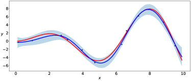
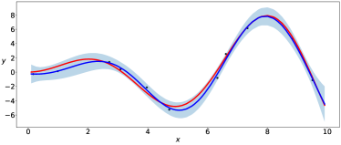
In the one-dim example, the data are generated from the test function $y(x)=x\sin(x)+\epsilon$ for $x\in[0,10]$ The size of the training and test data sets are $n=11$ and $m=100$, respectively. The variance of the noise is $\sigma^{2}=0.5^{2}$.

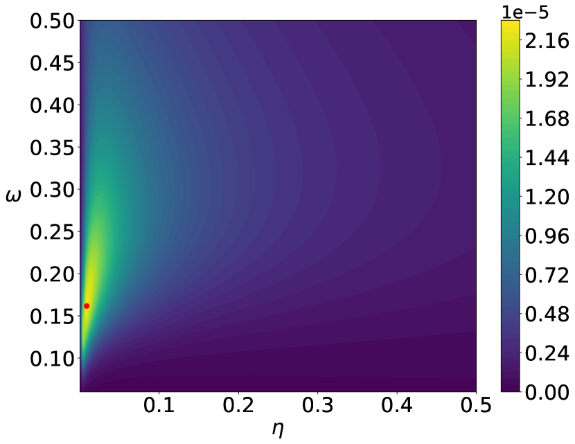
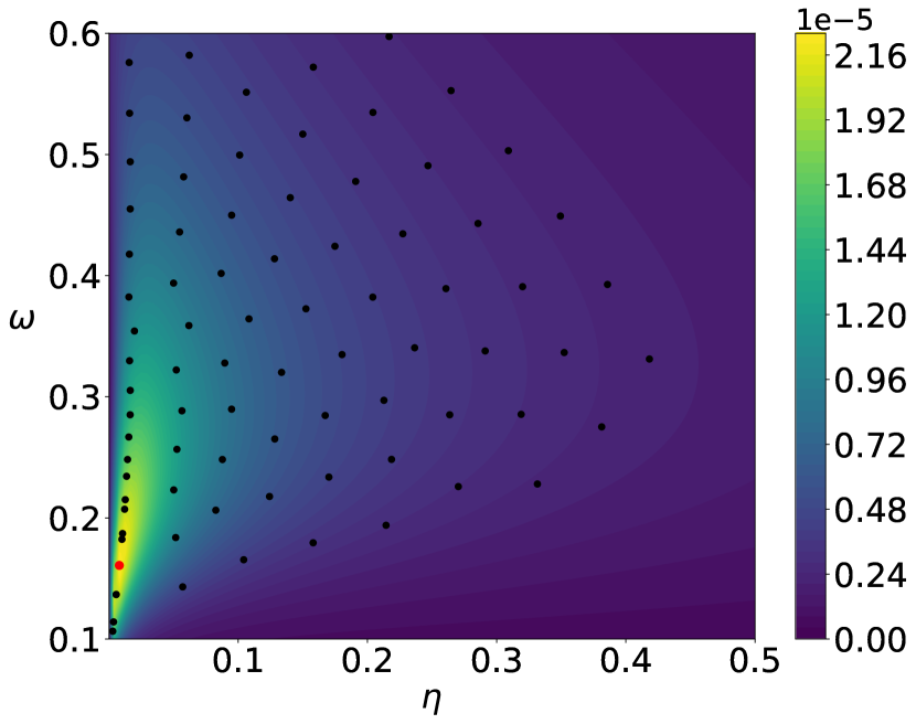
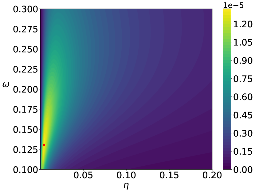
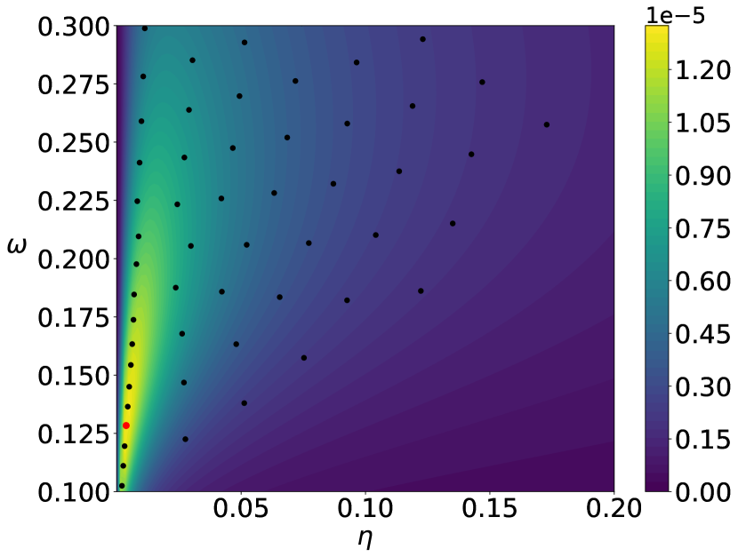
The parameters of the prior distributions of the EVI-GP are $a_{\omega}=a_{\eta}=1$, $b_{\omega}=b_{\eta}=0.5$, and $df_{\tau^{2}}=0$ which is equivalent to $p(\tau^{2})\propto 1/\tau^{2}$. We consider two possible mean functions for the GP model, the constant mean $\mu(x)=\beta_{0}$ and the linear mean $\mu(x)=\beta_{0}+\beta_{1}x$. There is no need for parameter regularization for these simple mean functions, and thus we use non-informative prior for $\bm{\beta}$. We use the EVI-post to approximate $p(\omega,\eta|\bm{y}_{n})$ and set the number of particles $N=100$, kernel bandwidth $h=0.02$ and stepsize $\tau=1$ in the EVI procedure. The initial particles are sampled from the uniform distribution in $[0,0.1]\times[0.1,0.4]$. Figure 1 and 2 show the posterior modes and particles returned by EVI-MAP and EVI-post, as well as the prediction and predictive confidence interval returned by both methods.

We compare the EVI-GP with three R packages. For the gpfit package, we set the nugget threshold to be $[0,25]$, corresponding to $\eta$ in our method, and the correlation is the Gaussian kernel function. For the mlegp package, we set the argument constMean to be 0 for the constant mean model and 1 for the linear mean model. The optimization-related arguments in mlegp are set as follows. The number of simplexes tries is 5. Each simplex maximum iteration is 5000. The relative tolerance is $1e^{-8}$, BFGS maximum iteration is 500, BFGS tolerance is $0.01$, and BFGS bandwidth is $1e^{-10}$. Other parameters in these two packages are set to default. For the laGP package, we set the argument start at 6, end at 10, d at null, g at $1e^{-4}$, method to a list of ”alc”, ”alcray”, ”mspe”, ”nn”, ”fish”, and Xi.ret at True. 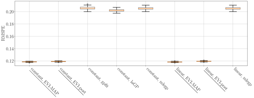The comparison in terms of prediction accuracy is shown in Table 1 and Figure 3. Table 1 shows the mean of RMSPEs from 100 simulations and Figure 3 shows the box plots of the RMSPEs. In the third column of Table 1, we only list the best result from the three R packages. The prediction accuracy of both versions of the EVI-GP performs almost equally well and both significantly outperform the three R packages.

We test the proposed method using the OTL-circuit function of input dimension $d=6$. The OTL-circuit function models an output transformerless push-pull circuit. The function is defined as follows,

where $V_{b1}=12R_{b2}/(R_{b1}+R_{b2})$, $R_{b1}\in[50,150]$ is the resistance of b1 (K-Ohms), $R_{b2}\in[25,70]$ is the resistance of b2 (K-Ohms), $R_{f}\in[0.5,3]$ is the resistance of f (K-Ohms), $R_{c1}\in[1.2,2.5]$ is the resistance of c1 (K-Ohms), $R_{c2}\in[0.25,1.2]$ is the resistance of c2 (K-Ohms) and $I\in[50,300]$ is the current gain (Amperes).

The size of training and testing datasets is 200 and 1000, respectively. We set the variance of the noise $\sigma^{2}=0.02^{2}$. For the prior distributions of $\bm{\omega}$, we let $\omega_{i}\overset{\text{i.i.d.}}{\sim}\text{Gamma}(a_{\omega}=1,b_{\omega}=2)$ for $i=2,\ldots,8$, but $\omega_{1}\sim\text{Gamma}(a_{\omega}=4,b_{\omega}=2)$. The prior distribution of $\eta\sim\text{Gamma}(a_{\eta}=1,b_{\eta}=2)$. Both non-informative and informative prior distributions are considered. When using the informative prior, we set $r=1/3$ and $df_{\tau^{2}}=7$ for the prior distribution of $\bm{\beta}$ and $\tau^{2}$. For the variance of the prior distribution of $\bm{\beta}$, we choose $\nu=4.35$, which was the result of 5-fold cross-validation when the biggest mean model is used. After variable selection, the 5-fold cross-validation is conducted again to find the optimal $\nu$ to fit the finalized GP model, which leads to $\nu=4.05$. In both cross-validation procedures, $\nu$ is searched in an evenly spaced grid from 0 to 5 with $0.05$ grid size.

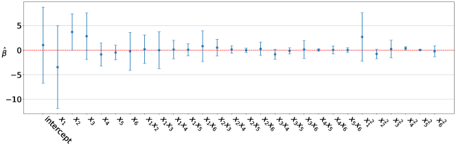
For both EVI-post and EVI-MAP, we set $h=0.001$ and $\tau=0.1$. For the EVI-post approach, we use $N=100$ particles, and the initial particles of $(\bm{\omega},\eta)$ are sampled uniformly in $[0,0.1]^{7}$. The two versions of EVI-GP perform very similarly, so we only return the result of EVI-MAP. The initial mean model of the GP is assumed as a quadratic function of the input variables, including the 2-way interactions. Based on the $95\%$ posterior confidence interval in Figure 4 of the $\bm{\beta}$, we select $x_{2}$ and $x_{2}^{2}$ as the significant terms to be kept for the final model.

For comparison, we choose the R package mlegp because only this package allows the specification of the mean model. We set the argument constMean to be 0 for the constant mean and 1 for the linear mean model. For the full quadratic mean model, we manually add all the second-order effect terms as the input and set constMean to 1. Unfortunately, the input of the mean and correlation cannot be separately specified in mlegp. So once we specify the mean part to have all the quadratic terms, the input of the correlation function also contains the quadratic terms. But we believe this might give more advantage for mlegp because the correlation involves more input variables. If some of the variables are not needed, their corresponding correlation parameter estimated by mlegp can be close to zero. The other arguments in mlegp are set in the same way as the previous example. 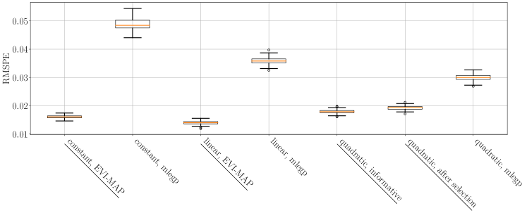Table 2 compares the mean of 100 standardized RMSPEs of the 100 simulations of EVI-GP and mlegp and Figure 5 shows the box plots of the RMSPEs of different models returned by the two methods. The EVI-GP is much more accurate than mlegp package in terms of prediction. However, for this example, variable selection does not improve the model in terms of prediction. The most accurate model is the GP with a linear function of the input variables as the mean model.

In this subsection, we test the EVI-GP with the famous Borehole function, which is defined as follows:

where $r_{\omega}\in[0.05,0.15]$ is the radius of the borehole (m), $r\in[100,50000]$ is the radius of influence (m), $T_{u}\in[63070,115600]$ is the transmissivity of the upper aquifer (m2/yr), $H_{u}\in[990,1110]$ is the potentiometric head of upper aquifer (m),$T_{l}\in[63.1,116]$ is the transmissivity of the lower aquifer (m2/yr), $H_{l}\in[700,820]$ is the potentiometric head of lower aquifer (m), $L\in[1120,1680]$ is the length of the borehole (m), $K_{\omega}\in[9855,12045]$ is the hydraulic conductivity of borehole (m/yr).

We use a training dataset of size 200 and 100 testing datasets of size 100. The noise variance is $\sigma^{2}=0.02^{2}$. We use the same parameter settings for the prior distributions and EVI-GP method as in the OTL-Circuit example. Regarding the variance of the prior distribution of $\bm{\beta}$, $\nu=4.55$ was the result of 5-fold cross-validation when the biggest mean model was used. After variable selection, the 5-fold cross-validation is conducted again to find the optimal $\nu$ to fit the finalized GP model. Coincidently, the optimal $\nu$ is also $4.55$. The initial mean model of the GP is assumed as a quadratic function of the input variables, including the 2-way interactions. 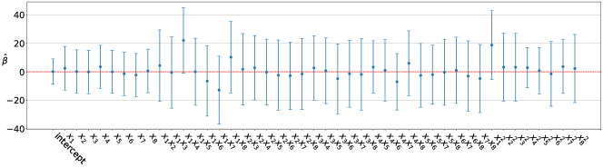Based on the $95\%$ posterior confidence interval in Figure 6 of the $\bm{\beta}$, we select intercept, $x_{1},x_{4}$, and $x_{1}x_{4}$ as the significant terms to be kept for the final model. 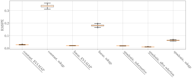Similarly, we compare the EVI-GP with the mlegp package, and the RMSPEs of the 100 simulations are shown in Table 3 and Figure 7. Again, EVI-GP is much better than the R package. More importantly, variable selection proves to be essential for the Borehole example, as the final GP model with the reduced mean model is more accurate than both the quadratic and linear mean models.

References

- Ai et al. (2009) Ai, M., Kang, L., and Joseph, V. R. (2009), “Bayesian optimal blocking of factorial designs,” Journal of Statistical Planning and Inference, 139, 3319–3328.
- Blei et al. (2017) Blei, D. M., Kucukelbir, A., and McAuliffe, J. D. (2017), “Variational inference: A review for statisticians,” Journal of the American statistical Association, 112, 859–877.
- Carnell (2022) Carnell, R. (2022), lhs: Latin Hypercube Samples, r package version 1.1.5.
- Cheng and Boots (2017) Cheng, C.-A. and Boots, B. (2017), “Variational Inference for Gaussian Process Models with Linear Complexity,” in Advances in Neural Information Processing Systems, eds. Guyon, I., Luxburg, U. V., Bengio, S., Wallach, H., Fergus, R., Vishwanathan, S., and Garnett, R., Curran Associates, Inc., vol. 30.
- Cressie (2015) Cressie, N. (2015), Statistics for spatial data, John Wiley & Sons.
- Dancik and Dorman (2008) Dancik, G. M. and Dorman, K. S. (2008), “mlegp: statistical analysis for computer models of biological systems using R,” Bioinformatics, 24, 1966–1967.
- E et al. (2020) E, W., Ma, C., and Wu, L. (2020), “Machine learning from a continuous viewpoint, I,” Science China Mathematics, 1–34.
- Fang et al. (2005) Fang, K.-T., Li, R., and Sudjianto, A. (2005), Design and modeling for computer experiments, CRC press.
- Gelman et al. (2014) Gelman, A., Carlin, J. B., Stern, H. S., Dunson, D. B., Vehtari, A., and Rubin, D. B. (2014), Bayesian Data Analysis, Third Edition, New York: Chapman and Hall/CRC.
- Ghanem et al. (2017) Ghanem, R., Higdon, D., and Owhadi, H. (2017), Handbook of uncertainty quantification, Springer.
- Giga et al. (2017) Giga, M.-H., Kirshtein, A., and Liu, C. (2017), “Variational Modeling and Complex Fluids,” in Handbook of Mathematical Analysis in Mechanics of Viscous Fluids, eds. Giga, Y. and Novotny, A., Springer International Publishing, pp. 1–41.
- Gramacy (2016) Gramacy, R. B. (2016), “laGP: Large-Scale Spatial Modeling via Local Approximate Gaussian Processes in R,” Journal of Statistical Software, 72, 1–46.
- Gramacy (2020) — (2020), Surrogates: Gaussian Process Modeling, Design and Optimization for the Applied Sciences, Boca Raton, Florida: Chapman Hall/CRC, http://bobby.gramacy.com/surrogates/.
- Gramacy and Apley (2015) Gramacy, R. B. and Apley, D. W. (2015), “Local Gaussian process approximation for large computer experiments,” Journal of Computational and Graphical Statistics, 24, 561–578.
- Gramacy and Lee (2008) Gramacy, R. B. and Lee, H. K. H. (2008), “Bayesian treed Gaussian process models with an application to computer modeling,” Journal of the American Statistical Association, 103, 1119–1130.
- Hamada and Wu (1992) Hamada, M. and Wu, C. J. (1992), “Analysis of designed experiments with complex aliasing,” Journal of quality technology, 24, 130–137.
- Joseph (2006) Joseph, V. R. (2006), “A Bayesian approach to the design and analysis of fractionated experiments,” Technometrics, 48, 219–229.
- Kang et al. (2023) Kang, L., Deng, X., and Jin, R. (2023), “Bayesian D-Optimal Design of Experiments with Quantitative and Qualitative Responses,” The New England Journal of Statistics in Data Science, 1–15.
- Kang and Huang (2019) Kang, L. and Huang, X. (2019), “Bayesian A-Optimal Design of Experiment with Quantitative and Qualitative Responses,” Journal of Statistical Theory and Practice, 13, 1–23.
- Kang and Joseph (2009) Kang, L. and Joseph, V. R. (2009), “Bayesian optimal single arrays for robust parameter design,” Technometrics, 51, 250–261.
- Kang et al. (2018) Kang, L., Kang, X., Deng, X., and Jin, R. (2018), “A Bayesian hierarchical model for quantitative and qualitative responses,” Journal of Quality Technology, 50, 290–308.
- Kang et al. (2021) Kang, X., Ranganathan, S., Kang, L., Gohlke, J., and Deng, X. (2021), “Bayesian auxiliary variable model for birth records data with qualitative and quantitative responses,” Journal of statistical computation and simulation, 91, 3283–3303.
- MacDonald et al. (2015) MacDonald, B., Ranjan, P., and Chipman, H. (2015), “GPfit: An R Package for Fitting a Gaussian Process Model to Deterministic Simulator Outputs,” Journal of Statistical Software, 64, 1–23.
- Neal (1996) Neal, R. M. (1996), Bayesian Learning for Neural Networks, New York, NY: Springer New York, chap. Monte Carlo Implementation, pp. 55–98.
- Onsager (1931a) Onsager, L. (1931a), “Reciprocal relations in irreversible processes. I.” Phys. Rev., 37, 405.
- Onsager (1931b) — (1931b), “Reciprocal relations in irreversible processes. II.” Phys. Rev., 38, 2265.
- Paszke et al. (2019) Paszke, A., Gross, S., Massa, F., Lerer, A., Bradbury, J., Chanan, G., Killeen, T., Lin, Z., Gimelshein, N., Antiga, L., Desmaison, A., Kopf, A., Yang, E., DeVito, Z., Raison, M., Tejani, A., Chilamkurthy, S., Steiner, B., Fang, L., Bai, J., and Chintala, S. (2019), “PyTorch: An Imperative Style, High-Performance Deep Learning Library,” in Advances in Neural Information Processing Systems 32, Curran Associates, Inc., pp. 8024–8035.
- Peng and Wu (2014) Peng, C.-Y. and Wu, C. F. J. (2014), “On the Choice of Nugget in Kriging Modeling for Deterministic Computer Experiments,” Journal of Computational and Graphical Statistics, 23, 151–168.
- Rasmussen and Williams (2006) Rasmussen, C. E. and Williams, C. K. I. (2006), Gaussian Processes for Machine Learning, Adaptive Computation and Machine Learning, MIT Press.
- Rayleigh (1873) Rayleigh, L. (1873), “Some General Theorems Relating to Vibrations,” Proceedings of the London Mathematical Society, 4, 357–368.
- Robert et al. (1999) Robert, C. P., Casella, G., and Casella, G. (1999), Monte Carlo statistical methods, vol. 2, Springer.
- Roberts and Rosenthal (1998) Roberts, G. O. and Rosenthal, J. S. (1998), “Optimal scaling of discrete approximations to Langevin diffusions,” Journal of the Royal Statistical Society: Series B (Statistical Methodology), 60, 255–268.
- Rockafellar (1976) Rockafellar, R. T. (1976), “Monotone operators and the proximal point algorithm,” SIAM J. Control Optim., 14, 877–898.
- Sacks et al. (1989) Sacks, J., Welch, W. J., Mitchell, T. J., and Wynn, H. P. (1989), “Design and Analysis of Computer Experiments,” Statistical Science, 4.
- Santner et al. (2003) Santner, T. J., Williams, B. J., Notz, W. I., and Williams, B. J. (2003), The design and analysis of computer experiments, vol. 1, Springer.
- Surjanovic and Bingham (2013) Surjanovic, S. and Bingham, D. (2013), “Virtual Library of Simulation Experiments: Test Functions and Datasets,” Retrieved October 1, 2023, from http://www.sfu.ca/~ssurjano.
- Tran et al. (2016) Tran, D., Ranganath, R., and Blei, D. M. (2016), “The variational Gaussian process,” in 4th International Conference on Learning Representations, ICLR 2016.
- Trillos and Sanz-Alonso (2020) Trillos, N. G. and Sanz-Alonso, D. (2020), “The Bayesian Update: Variational Formulations and Gradient Flows,” Bayesian Analysis, 15, 29 – 56.
- Wang et al. (2021) Wang, Y., Chen, J., Liu, C., and Kang, L. (2021), “Particle-based energetic variational inference,” Statistics and Computing, 31, 1–17.
- Wu and Hamada (2021) Wu, C. J. and Hamada, M. S. (2021), Experiments: planning, analysis, and optimization, Hoboken, NJ: John Wiley & Sons, Inc.
- Wynne and Wild (2022) Wynne, G. and Wild, V. (2022), “Variational gaussian processes: A functional analysis view,” in International Conference on Artificial Intelligence and Statistics, PMLR, pp. 4955–4971.