Energetics and Efimov states of three interacting bosons and mass-imbalanced fermions in a three-dimensional spherical harmonic trap

By expressing the relative wavefunction as an expansion over basis states it is possible to obtain the allowable energy states for any value of $a_{\rm s}$ via a matrix eigenvalue problem Liu et al. (2009); Kestner and Duan (2007); Liu et al. (2010). Due to the separability of the centre-of-mass and relative Hamiltonians the total three-body wavefunction may be written

$\displaystyle\Psi_{\rm 3b}(\vec{C},\vec{r},\vec{\rho})=\chi_{\rm COM}(\vec{C})\psi_{\rm 3b}^{\rm rel}(\vec{r},\vec{\rho}).$

(9)

The centre of mass wavefunction, $\chi_{\rm COM}(\vec{C})$, is a SHO wavefunction of lengthscale $a_{\rm COM}$. The relative wavefunction, $\psi_{\rm 3b}^{\rm rel}(\vec{r},\vec{\rho})$, can be written

	$\displaystyle\psi_{\rm 3b}^{\rm rel}(\vec{r},\vec{\rho})$	$\displaystyle=$
	$\displaystyle(1+\hat{Q})$	$\displaystyle\sum_{n=0}^{\infty}C_{n}\psi_{\rm 2b}^{\rm rel}\left(\nu_{nl},\frac{r}{a_{\mu}}\right)R_{nl}\left(\frac{\rho}{a_{\mu}}\right)Y_{lm}(\hat{\rho}),$

where $\psi_{\rm 2b}^{\rm rel}$ is the relative interacting two-body wavefunctions, first derived by Ref. Busch et al. (1998), and $\nu_{nl}$ are the energy pseudo-quantum numbers. $R_{nl}$ is the normalisation and radial part of the three dimensional SHO wavefunction and $Y_{lm}$ is the spherical harmonic. $\hat{Q}$ is the symmetrisation operator, it ensures the correct bosonic or fermionic symmetry of the wavefunction. For three identical bosons $\hat{Q}=\hat{P}_{13}+\hat{P}_{23}$, for two identical fermions and one distinct particle $\hat{Q}=-\hat{P}_{23}$, where $\hat{P}_{jk}$ exchanges the location of particles $j$ and $k$. The $C_{n}$ terms are coefficients of expansion.

The energy of $\psi_{\rm 3b}^{\rm rel}$ is given by

$\displaystyle E_{\rm rel}=(2\nu_{nl}+2n+l+3)\hbar\omega,$

(11)

where $\nu_{nl}+n$ is constant so that the energy of each term in Eq. (LABEL:eq:psi1) is the same.

The explicit form of the relative two-body wavefunction is Busch et al. (1998)

	$\displaystyle\psi_{\rm 2b}^{\rm rel}\left(\nu_{nl},\tilde{r}\right)=N_{\nu_{nl}}e^{-\tilde{r}^{2}/2}\Gamma(-\nu_{nl})U\left(-\nu_{nl},\frac{3}{2},\tilde{r}^{2}\right),$		(12)
	$\displaystyle N_{\nu_{nl}}=\sqrt{\frac{\nu_{nl}\Gamma(-\nu_{nl}-1/2)}{2\pi^{2}a_{\mu}^{3}\Gamma(1-\nu_{nl})[\psi^{(0)}(-\nu_{nl}-1/2)-\psi^{(0)}(-\nu_{nl})]}},$

where $U$ is Kummer’s function, $\tilde{r}=r/a_{\mu}$ and $\psi^{(0)}$ is the digamma function of degree 0. The explicit form of $R_{nl}$ is given by

	$\displaystyle R_{nl}\left(\tilde{\rho}\right)$	$\displaystyle=$	$\displaystyle N_{nl}\left(\tilde{\rho}\right)^{l}e^{-\tilde{\rho}^{2}/2}L_{n}^{l+\frac{1}{2}}\left(\tilde{\rho}^{2}\right),$		(13)
	$\displaystyle N_{nl}$	$\displaystyle=$	$\displaystyle\sqrt{\sqrt{\frac{1}{4\pi a_{\mu}^{6}}}\frac{2^{n+l+3}n!}{(2n+2l+1)!!}},$

where $L_{n}^{l+\frac{1}{2}}$ is the associated Laguerre polynomial, and $\tilde{\rho}=\rho/a_{\mu}$. The exchange operators are given by

	$\displaystyle\hat{P}_{23}$		$\displaystyle f(\vec{C},\vec{r},\vec{\rho})$
			$\displaystyle=f\left(\vec{C},\frac{m\vec{r}}{m+m_{\rm i}}+\gamma\vec{\rho},\frac{(2m+m_{\rm i})m_{\rm i}\vec{r}}{(m+m_{\rm i})^{2}\gamma}-\frac{m\vec{\rho}}{m+m_{\rm i}}\right),$

where $m=m_{2}=m_{3},\quad m_{1}=m_{\rm i}$ and

	$\displaystyle\hat{P}_{13}$		$\displaystyle f(\vec{C},\vec{r},\vec{\rho})$
			$\displaystyle=f\left(\vec{C},\frac{m_{i}\vec{r}}{m+m_{\rm i}}-\gamma\vec{\rho},\frac{-(2m+m_{\rm i})m_{\rm i}\vec{r}}{(m+m_{\rm i})^{2}\gamma}-\frac{m\vec{\rho}}{m+m_{\rm i}}\right),$

where $m=m_{1}=m_{3},\quad m_{\rm i}=m_{2}$. In this paper $\hat{P}_{13}$ is only applicable to the bosonic case where $m_{1}=m_{2}=m_{3}=m_{\rm i}=m$.

As per Refs. Liu et al. (2009, 2010) the allowable values of the scattering length and expansion coefficients for a chosen energy (and thus chosen $\nu_{nl}$) can be determined from the following matrix equation,

$\displaystyle\frac{a_{\mu}}{a_{\rm s}}\begin{bmatrix}C_{0}\\ C_{1}\\ \vdots\end{bmatrix}=\begin{bmatrix}X_{00l}&X_{01l}&X_{02l}&\dots\\ X_{10l}&X_{11l}&X_{12l}&\dots\\ \vdots&\vdots&\vdots&\ddots\\ \end{bmatrix}\begin{bmatrix}C_{0}\\ C_{1}\\ \vdots\end{bmatrix},$

(16)

where

$\displaystyle X_{n^{\prime}nl}=\frac{2\Gamma(-\nu_{n^{\prime}l})}{\Gamma(-\nu_{n^{\prime}l}-\frac{1}{2})}\delta_{n^{\prime}n}-\eta\frac{(-1)^{l}}{\sqrt{\pi}}A_{n^{\prime}nl},$

(17)

and

	$\displaystyle A_{n^{\prime}nl}=\frac{a_{\mu}^{3}}{N_{\nu_{nl}}}\int_{0}^{\infty}\tilde{\rho}^{2}R_{n^{\prime}l}(\tilde{\rho})R_{nl}\left(\frac{\kappa\tilde{\rho}}{1+\kappa}\right)$
	$\displaystyle\times\psi_{\rm 2b}^{\rm rel}\left(\nu_{nl},\sqrt{\frac{2\kappa+1}{(1+\kappa)^{2}}}\tilde{\rho}\right)d\tilde{\rho},$		(18)

and $\eta=-1$ or $\eta=2$ for the fermionic and bosonic cases respectively. With Eqs. (16)–(18) the energy spectrum of the relative three-body wavefunction can be calculated for any desired value of $\kappa$.

Additionally in the $\kappa\rightarrow 0$ limit (the heavy-impurity limit) the matrix elements can be determined analytically:

$\displaystyle A_{n^{\prime}n,l}=\begin{cases}\dfrac{2}{n^{\prime}-\nu}\sqrt{\dfrac{\Gamma(n+3/2)\Gamma(n^{\prime}+3/2)}{\pi\Gamma(n+1)\Gamma(n^{\prime}+1)}}&l=0\\ \quad 0&l>0\end{cases}.\quad\quad$

(19)

However in the heavy substrate limit, $\kappa\rightarrow\infty$, Eq. (18) diverges due to to $\psi_{\rm 2b}^{\rm rel}(\nu,r)$ diverging as $r\rightarrow 0$. It should be noted that the $\kappa\rightarrow\infty$ limit can be evaluated using the Born-Oppenheimer approximation Petrov (2012).

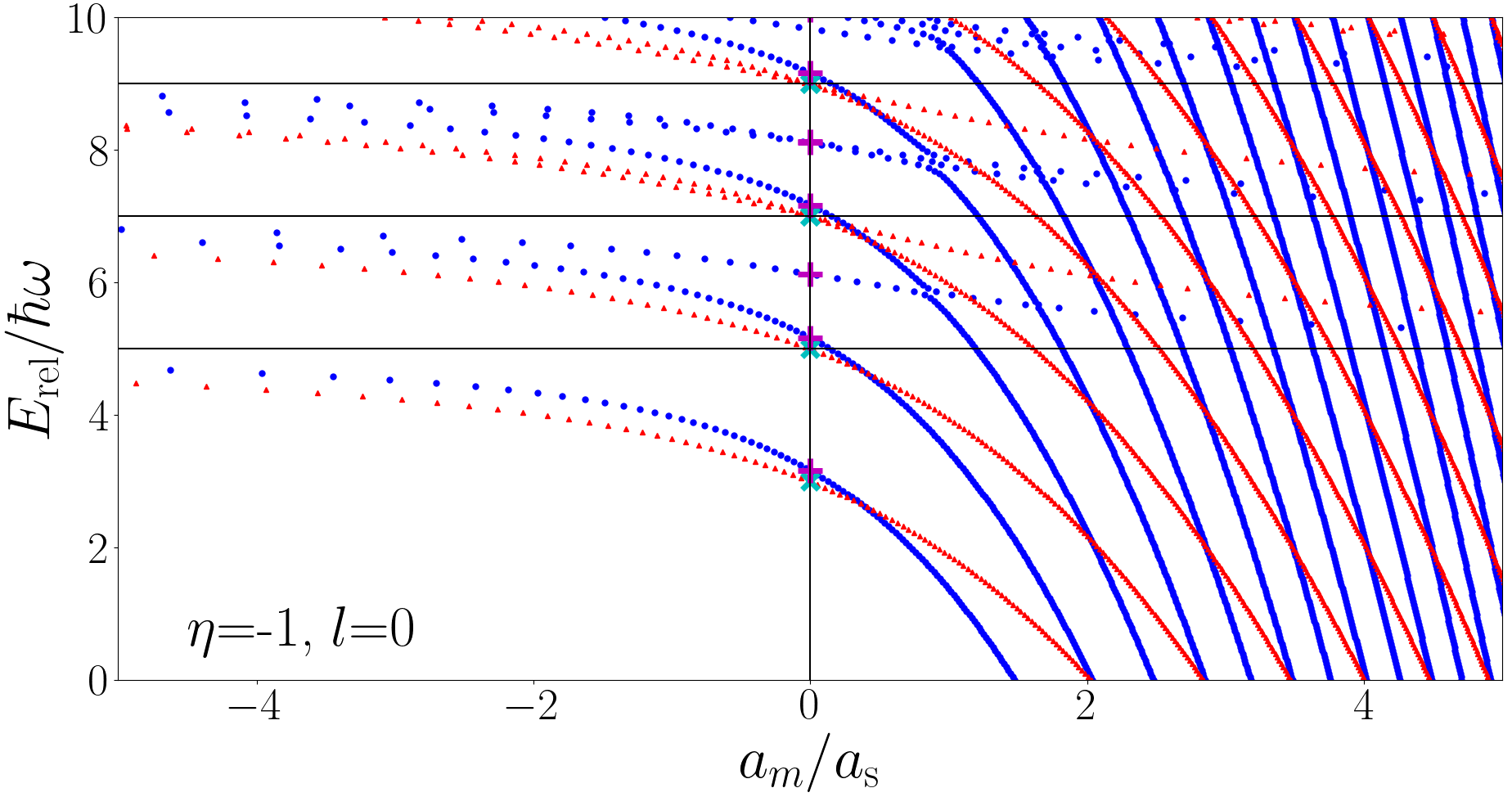
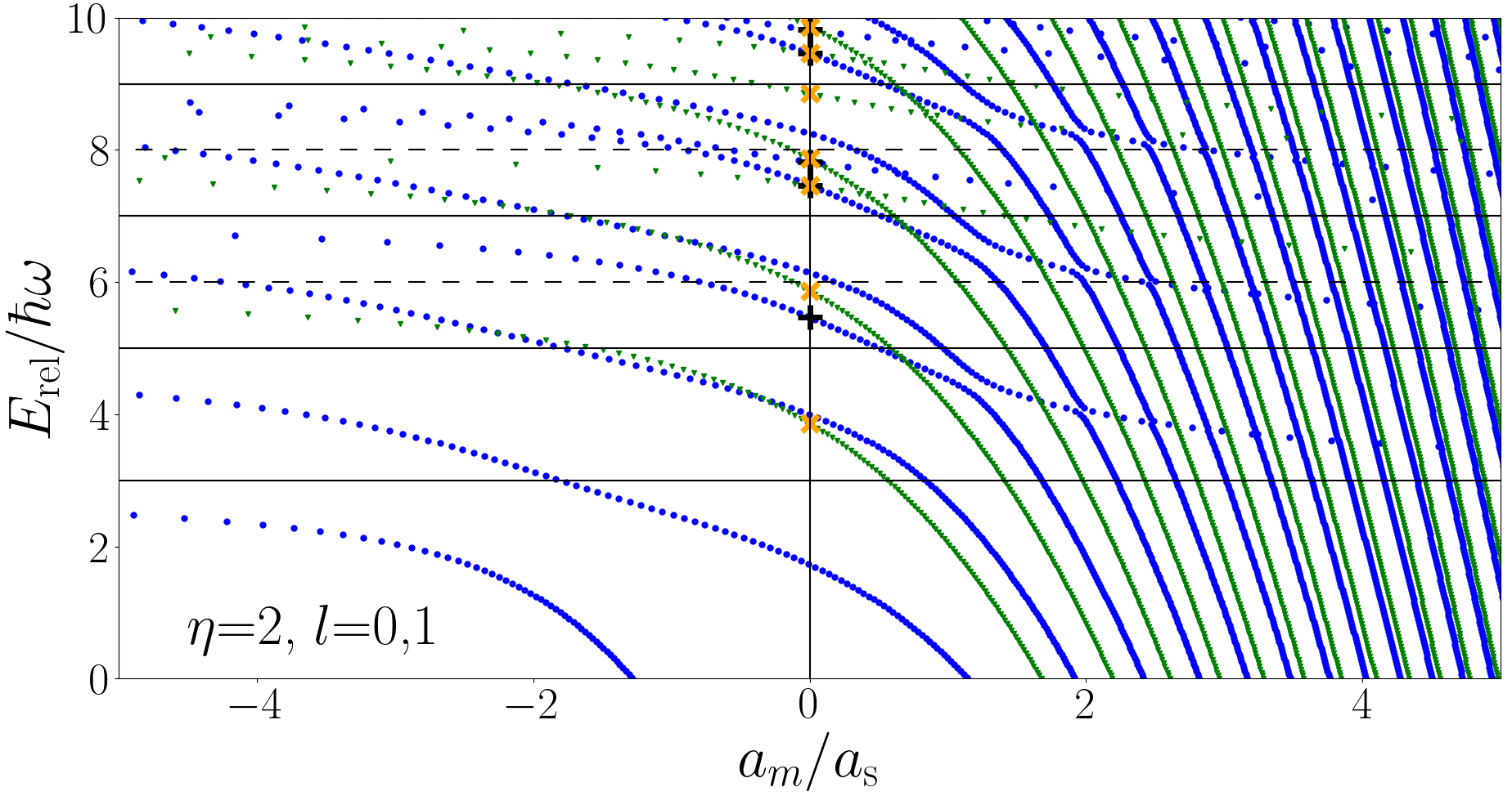
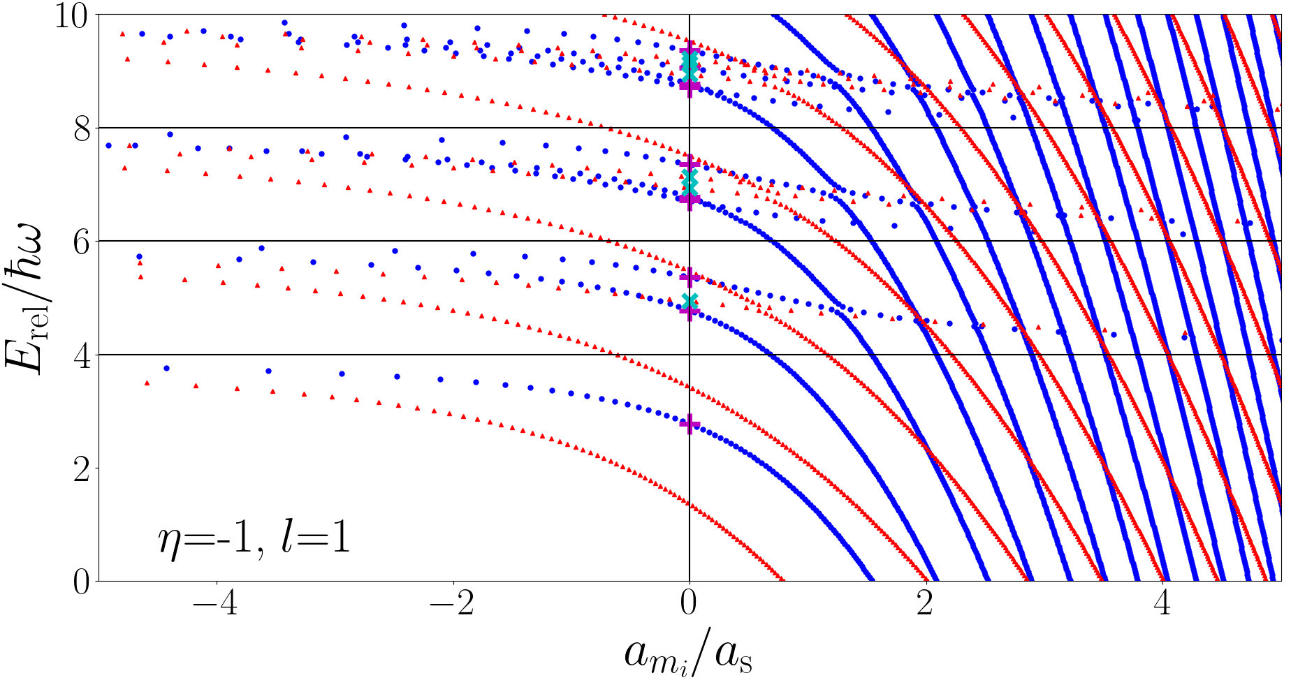
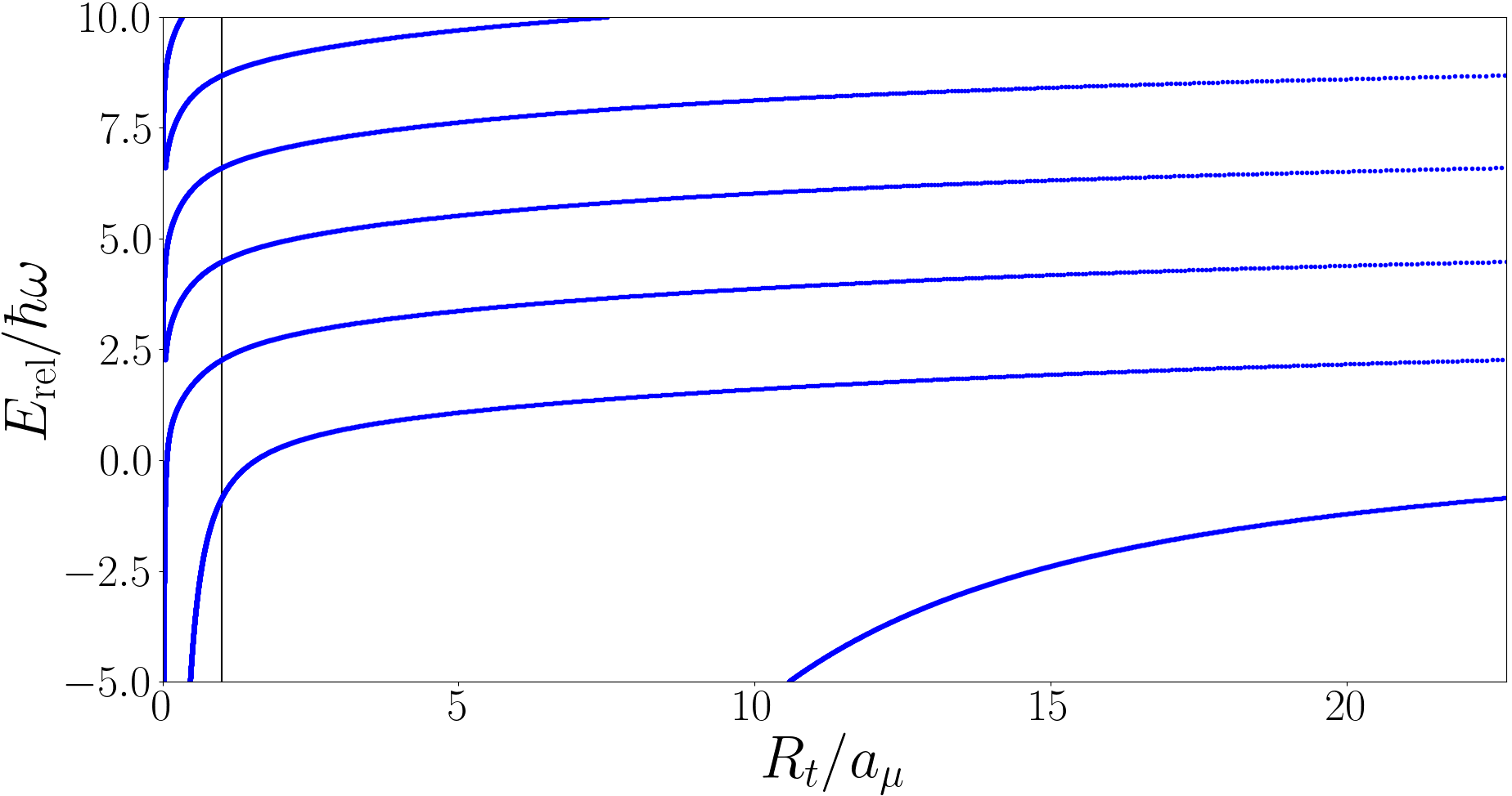
The three-body energy spectrum is given in Figs. 1, 2, and 3. In Fig. 1 we present the fermionic energy spectrum for $\kappa\rightarrow 0$ with $l=0$, for comparison, we also show our results for $\kappa=1$, which reproduce the results of Refs. Liu et al. (2010, 2009). In Fig. 2 we present the bosonic energy spectrum for $l=0$ and $l=1$, recall $\kappa=1$ for three identical bosons. In Fig. 3 we present the fermionic energy spectrum for $\kappa=1$ and $\kappa=13.75$ with $l=1$. In all figures the horizontal black lines define the non-interacting energies and the vertical black lines are simply to indicate unitarity $(a_{\rm s}\rightarrow\infty)$.

In Fig 1 we observe for $\kappa=1$ and $a_{\rm s}^{-1}>0$ sharp and close anticrossings are present which make it difficult to clearly identify which unitary states ultimately diverge and which converge as $a_{\rm s}^{-1}\rightarrow+\infty$. However in the $\kappa\rightarrow 0$ limit these anticrossings disappear. This makes the identification of which states are ultimately divergent and convergent much more reliable. Notice that for every unitary energy there is one divergent state and the multiplicity at unitarity increases by one every $4\hbar\omega$. This is consistent with Eq. (33) in Section II.2 and implies that the $s_{00}$ states (see Section II.2), and only the $s_{00}$ states, are divergent as $a_{\rm s}\rightarrow+0$. This is similar to findings of Ref. Liu et al. (2010) for the $\kappa=1$ case where the $s_{n=0,l}$ states are identified as the divergent states.

In Fig. 2, the bosonic case, we observe many of the same features as the fermionic spectra in Fig. 1. Again all states converge to non-interacting energies for $a_{\rm s}^{-1}\rightarrow-\infty$ but for $a_{\rm s}^{-1}\rightarrow+\infty$ there are both divergent and convergent states, additionally anticrossings are present. For $l=0$ we are able to identify the $s_{10}$ states as being divergent in the $a_{\rm s}^{-1}\rightarrow+\infty$, however, unlike the $l=0$ fermion spectra discussed above, these are not the only divergent states, all Efimov states (discussed in Section II.3) are divergent in the $a_{\rm s}^{-1}\rightarrow+\infty$ limit. For $l=1$, anticrossings are still present but fewer in number and narrower. The lowest $s_{n=0,l}$ states being divergent no longer appears to be true, the $(q,s_{11})=(0,6.462\dots)$ state is divergent and the $(q,s_{01})=(2,2.864\dots)$ state is not divergent.

In Fig. 3 for $\kappa=13.75$ we again observe anticrossings and that the states corresponding to the smallest real value of $s_{nl}$ diverge as $a_{\rm s}^{-1}\rightarrow+\infty$. However, unlike the bosonic case some, but curiously not all, Efimov states diverge as $a_{\rm s}^{-1}\rightarrow+\infty$. Only the lowest three Efimov energies are divergent in this limit.

In Section II.1 we have derived the three-body relative wavefunction for general s-wave scattering length, $a_{\rm s}$, and general mass ratio, $\kappa$, in the form of an infinite sum, Eq. (LABEL:eq:psi1). However, it is possible to derive a closed form eigenfunction of $\hat{H}_{\rm rel}$ using hyperspherical coordinates Werner and Castin (2006a); Werner (2008). Only in the unitary and non-interacting cases can the wavefunction be fully specified. Enforcing the Bethe-Peierls boundary condition leads to a transcendental equation that can be solved for one of the quantum numbers, $s_{nl}$, in the non-interacting and unitary regimes.

We define the hyperradius, $R$, and the hyperangle, $\alpha$,

$\displaystyle R=\sqrt{r^{2}+\rho^{2}},\quad\alpha=\arctan(\frac{r}{\rho}).$

(20)

In turn the relative Hamiltonian is given by

	$\displaystyle\hat{H}_{\rm rel}$	$\displaystyle=$	$\displaystyle\frac{-\hbar^{2}}{2\mu}\Bigg{[}\frac{\partial^{2}}{\partial R^{2}}+\frac{5}{R}\frac{\partial}{\partial R}+\frac{4}{R^{2}}$		(21)
			$\displaystyle+\frac{1}{R^{2}\sin^{2}(\alpha)\cos^{2}(\alpha)}\frac{\partial^{2}}{\partial\alpha^{2}}\Big{(}\cos(\alpha)\sin(\alpha)\mathchoice{\mathbin{\vbox{\hbox{\scalebox{0.5}{$\displaystyle\bullet$}}}}}{\mathbin{\vbox{\hbox{\scalebox{0.5}{$\textstyle\bullet$}}}}}{\mathbin{\vbox{\hbox{\scalebox{0.5}{$\scriptstyle\bullet$}}}}}{\mathbin{\vbox{\hbox{\scalebox{0.5}{$\scriptscriptstyle\bullet$}}}}}\Big{)}$
			$\displaystyle-\frac{\hat{\Lambda}^{2}_{\rho}}{R^{2}\cos^{2}(\alpha)}-\frac{\hat{\Lambda}^{2}_{r}}{R^{2}\sin^{2}(\alpha)}\Bigg{]}+\frac{\mu\omega^{2}R^{2}}{2},$

where $\hat{\Lambda}^{2}_{\rho}$ and $\hat{\Lambda}^{2}_{r}$ are the angular part of the three-dimensional Laplace operators acting on the $\hat{\rho}$ and $\hat{r}$ coordinate spaces respectively. In the unitary and non-interacting limits we can express the wavefunction in closed form. The unnormalised wavefunction is of the form

$\displaystyle\psi_{\rm 3b}^{\rm rel}$

$\displaystyle=$

$\displaystyle\frac{a_{\mu}^{2}}{R^{2}}F_{qs_{nl}}(R)(1+\hat{Q})\frac{\varphi_{ls_{nl}}(\alpha)}{\sin(2\alpha)}Y_{lm}(\hat{\rho}).$

(22)

Here $q$, $l$ and $s_{nl}$ are quantum numbers and give the energy

$\displaystyle E_{\rm rel}=(2q+l+s_{nl}+1)\hbar\omega.$

(23)

While $q$ and $l$ are non-negative integers the $s_{nl}$ quantum number is more complicated. Following the work of Refs. Werner and Castin (2006a); Liu et al. (2010) several conditions can be placed on the wavefunction:

	$\displaystyle\varphi_{ls_{nl}}\left(\frac{\pi}{2}\right)$	$\displaystyle=$	$\displaystyle 0,$		(24)
	$\displaystyle s^{2}\varphi_{ls_{nl}}(\alpha)$	$\displaystyle=$	$\displaystyle-\varphi_{ls_{nl}}^{\prime\prime}(\alpha)+\frac{l(l+1)}{\cos^{2}(\alpha)}\varphi_{ls_{nl}}(\alpha),$		(25)
	$\displaystyle E_{\rm rel}F_{qs_{nl}}(R)$	$\displaystyle=$	$\displaystyle\frac{-\hbar^{2}}{2\mu}\left(F_{qs_{nl}}^{\prime\prime}(R)+\frac{F_{qs_{nl}}^{\prime}(R)}{R}\right)$		(26)
			$\displaystyle+\left(\frac{\hbar^{2}s_{nl}^{2}}{2\mu R^{2}}+\frac{\mu\omega^{2}R^{2}}{2}\right)F(R).$

The first is enforced because a divergence at $\alpha=\pi/2$ is non-physical, the second and third come from requiring that Eq. (22) is an eigenfunction of Eq. (21). These conditions determine the functional form of the wavefunction. The hyperspherical solutions are given Liu et al. (2010)

			$\displaystyle\varphi_{ls_{nl}}(\alpha)=$
			$\displaystyle\cos^{l+1}(\alpha){}_{2}F_{1}\left(\frac{l+1-s_{nl}}{2},\frac{l+1+s_{nl}}{2};l+\frac{3}{2};\cos^{2}(\alpha)\right),$
	$\displaystyle F$		$\displaystyle(R)=\left(\frac{R}{a_{\mu}}\right)^{s_{nl}}e^{-R^{2}/2a_{\mu}^{2}}L_{q}^{s_{nl}}\left(\frac{R^{2}}{a_{\mu}^{2}}\right),$		(28)

where ${}_{2}F_{1}$ is the Gaussian hypergeometric function. This solution for $F(R)$ is valid for $s_{nl}^{2}\geq 0$. For $s_{nl}^{2}<0$ there is a different solution, see Section II.3. Note that some values of $s_{nl}$ and $l$ are forbidden and are not predicted by the method of Section II.1; $l=0$, $s=2$ for fermions and, $l=1$, $s=3$ and $l=0$, $s=4$ for bosons are forbidden because the wavefunctions are 0 Werner (2008).

The interactions are enforced by the Bethe-Peierls boundary condition, Eq. (8), and this allows for the values of $s_{nl}$ to be calculated, but only in the non-interacting and unitary regimes. In the intermediate regime this formalism breaks down. Note in Eq. (26) $s_{nl}^{2}$ appears not $s_{nl}$. Hence there is a degree of arbitrarity in $s_{nl}$, convention is to choose $s_{nl}\in[0,\infty)$ for $s_{nl}^{2}\geq 0$ and $s_{nl}\in i\cdot[0,\infty)$ for $s_{nl}^{2}<0$. The $s_{nl}^{2}<0$ case will be considered in more detail in Section II.3.

In the non-interacting case Eq. (8) implies $\varphi_{ls_{nl}}(0)=0$, and so the values of $s_{nl}$ are given Liu et al. (2010)

	$\displaystyle{\rm NI\;fermions\;}s_{nl}=\begin{cases}2n+4&l=0\\ 2n+l+2&l>0\end{cases},$		(29)
	$\displaystyle{\rm NI\;bosons\;}s_{nl}=\begin{cases}2&l=0\\ 2n+6&l=0\\ 2n+l+4&l=1\\ 2n+l+2&l>1\end{cases},$		(30)

where $n\in\mathbb{Z}_{\geq 0}$.

In the unitary limit $s_{nl}$ will solve the following transcendental equation

			$\displaystyle 0=$
			$\displaystyle\frac{d\varphi_{ls_{nl}}}{d\alpha}\Big{|}_{\alpha=0}+\eta(-1)^{l}\frac{(1+\kappa)^{2}}{\kappa\sqrt{1+2\kappa}}\varphi_{ls_{nl}}\left(\arctan(\frac{\sqrt{1+2\kappa}}{\kappa})\right).$
					(31)

See Table 1 for solutions to Eq. (31).

In the $\kappa\rightarrow 0$ limit, with $\eta=-1$ (fermions), Eq. (31) reduces to

$\displaystyle 0=\frac{d\varphi_{ls_{nl}}}{d\alpha}\Big{|}_{\alpha=0}-\delta_{l,0},$

(32)

in turn this implies, for $\kappa\rightarrow 0$,

$\displaystyle s_{nl}=\begin{cases}4n+2&l=0\\ 2n+l+1&l>0\end{cases},\quad$

(33)

where $n\in\mathbb{Z}_{\geq 0}$. Note $l=0$, $s=2$ is normally forbidden but because $s\rightarrow 2$ as $\kappa\rightarrow 0$ this is never violated for finite mass imbalance. In the $\kappa\rightarrow\infty$ limit the right-hand term in Eq. (31) diverges unless $s_{nl}$ takes specific values that cause the $\varphi_{ls_{nl}}$ part of the term to be 0. This implies, for $\kappa\rightarrow\infty$

$\displaystyle s_{nl}=\begin{cases}2n+4&l=0\\ 2n+l+2&l>0\end{cases},\quad$

(34)

where $n\in\mathbb{Z}_{\geq 0}$.

The energies at unitarity are plotted in Figs. 1, 2 and 3. In Fig. 1 the purple pluses indicate unitary energies for the $\kappa=1$ case and the cyan crosses for the $\kappa\rightarrow 0$ case. In Fig. 2 the black pluses indicate the unitary energies for $l=0$ and the orange crosses for $l=1$. In Fig. 3 the purple pluses indicate unitary energies for the $\kappa=1$ case and the cyan crosses for $\kappa=13.75$.

The energies calculated using the general method of Section II.1 are in excellent agreement with the hyperspherical approach of this section. However, as noted in the captions of Figs. 2 and 3, some states are not marked at unitarity with an energy from a hyperspherical calculation. These states are Efimov states and they correspond to the case where $s_{nl}$ is imaginary. In this case Eq. (28) is not the correct wavefunction and so $E_{\rm rel}=(2q+s_{nl}+1)\hbar\omega$ is not applicable.

The previous two sections have investigated the agreement between two different methods of calculating the unitary energy spectrum of trapped three-body systems including for bosons and the effects of mass imbalance. We find that the two methods are in excellent agreement, however, as noted in Figs. 2 and 3, there are some unitary energies predicted by the method of Section II.1 that are not predicted by Eqs. (23) and (31). These unmarked states, associated with imaginary values of $s_{nl}$, are Efimov states, e.g. $s_{00}$ for bosons and $s_{01}$ for $\kappa=13.75$ fermions.

Eq. (26) is the Schrödinger equation for a particle moving in a two dimensions with two potential terms, a harmonic potential and a term proportional to $s_{nl}^{2}/R^{2}$. If $s_{nl}$ is purely imaginary then this potential is attractive at short distances rather than repulsive. This necessitates a different class of solution compared to the case where $s_{nl}$ is purely real and these solutions are Efimov states. Physically speaking the Efimov effect is short-range interparticle interactions giving rise to an effective attractive long-range interaction due to a third particle mediating the effective interaction between the other two.

These states were first studied in Ref. Efimov (1971) in the free context and Ref. Jonsell et al. (2002) in a trapped context. Efimov states were first observed in an ultracold gas in Ref. Kraemer et al. (2006).

For imaginary $s_{nl}$ the hyperradial solution is given by Werner and Castin (2006a)

$\displaystyle F(R)=\frac{a_{\mu}}{R}W_{\dfrac{E_{\rm rel}}{2\hbar\omega},\dfrac{s_{nl}}{2}}\left(\frac{R^{2}}{a_{\mu}^{2}}\right),$

(35)

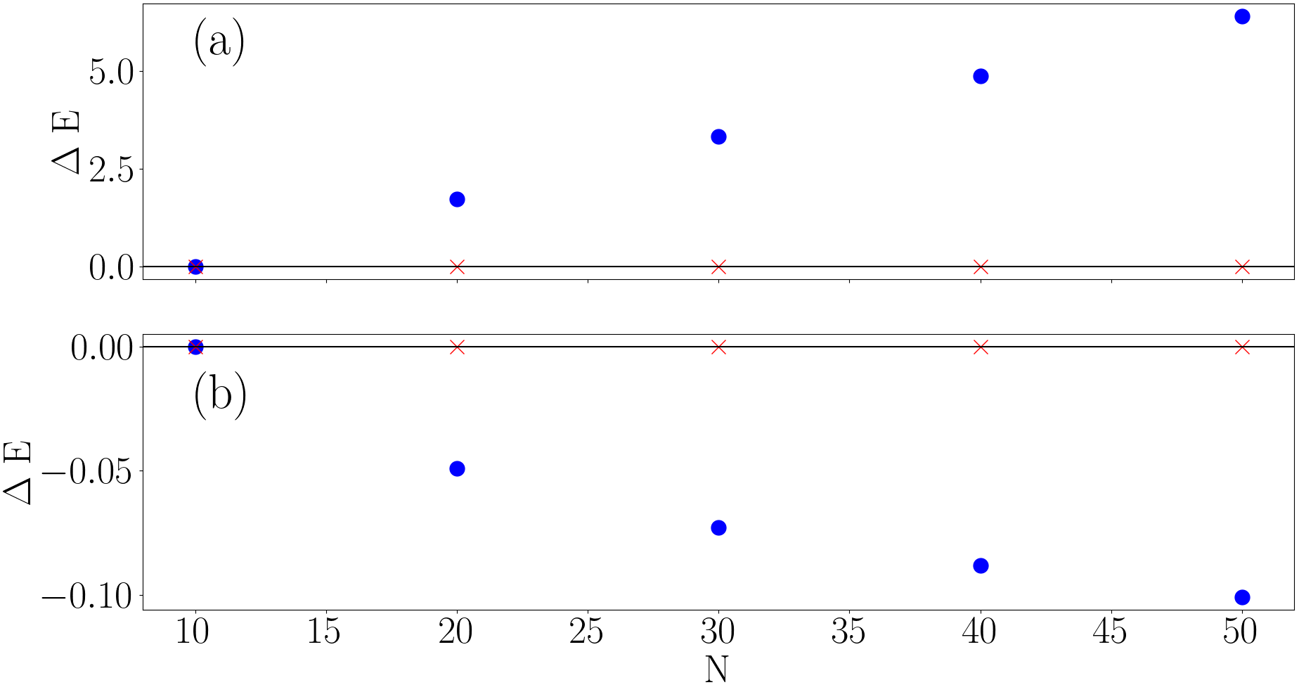
where $W_{a,b}(x)$ is the Whittaker function. In the universal ($s_{nl}^{2}\geq 0$) case Eqs. (26) and (28) imply $E_{\rm rel}=(2q+s_{nl}+1)\hbar\omega$. However, in the Efimov case the relative energy is left a free parameter. Using the method of Section II.1 the energies of the Efimov states do not converge to a constant value as the matrix size is increased, whereas the universal states do converge. This non-convergence of the Efimov states is shown in Fig. 4, where the change in energy, $\Delta E=(E-E_{N=10})/E_{N=10}$ is plotted as a function of the matrix size $(N)$ in Eq. (16). Figs. 4$(\rm a)$ and 4$(\rm b)$ plot $\Delta E$ for bosons and fermions respectively. From these plots it is clear that as $N$ is increased the energy for the universal states ($s_{nl}^{2}>0$) states remains constant, whereas the Efimov state energies diverge. This divergence arises from the fact that the Hamiltonian and Bethe-Peierls boundary condition do not contain enough information to uniquely specify the energies of the Efimov states. We find that the Efimov energies diverge logarithmically with $N$. As such an additional boundary condition is needed to fix the Efimov energies.

The Efimov hyperradial function, Eq. (35), oscillates increasingly rapidly as $R/a_{\mu}\rightarrow 0$ (but remains bounded). To find the Efimov states we require the phase of the oscillation to be fixed, and impose the boundary condition

$\displaystyle F(R)\underset{R\rightarrow 0}{=}A\sin[|s_{0l}|\ln(\frac{R}{a_{\mu}})-|s_{0l}|\ln(\frac{R_{t}}{a_{\mu}})\Big{]},$

(36)

where $A$ is a constant and $R_{t}>0$ is the three-body parameter. The short range behaviour of the Efimov hyperradial wavefunction is given by

	$\displaystyle\dfrac{a_{\mu}}{R}W_{\dfrac{E}{2\hbar\omega},\dfrac{s_{0l}}{2}}$		$\displaystyle\left(\dfrac{R^{2}}{a_{\mu}^{2}}\right)\underset{R\rightarrow 0}{=}$
			$\displaystyle\dfrac{\Gamma[-s_{0l}]}{\Gamma\left[\dfrac{1-s_{0l}-E/\hbar\omega}{2}\right]}\left(\dfrac{R}{a_{\mu}}\right)^{s_{0l}}$
			$\displaystyle+\dfrac{\Gamma[s_{0l}]}{\Gamma\left[\dfrac{1+s_{0l}-E/\hbar\omega}{2}\right]}\left(\dfrac{R}{a_{\mu}}\right)^{-s_{0l}}.$

From this we can derive a transcendental equation that determines the energy spectrum as a function of $R_{t}$ Jonsell et al. (2002)

$\displaystyle-|s_{0l}|\ln\left(\frac{R_{t}}{a_{\mu}}\right)$

$\displaystyle=$

$\displaystyle\arg\left\{\frac{\Gamma\left[\dfrac{1+s_{0l}-E}{2}\right]}{\Gamma[1+s_{0l}]}\right\}\quad{\rm mod}\;\pi.\qquad$

(38)

The energy spectrum is unbounded from above and below. We index the states with $q\in\mathbb{Z}$, and define the $q=0$ state to be the first positive energy state at $R_{t}/a_{\mu}=\exp(\pi/|s_{0l}|)$ with $q>0$ referring to higher energy states and $q<0$ to lower energy states. For example for $R_{t}/a_{\mu}=1$ and $s_{0l}=i\cdot 1.006$, the energies corresponding to $q=3,2,1,0,-1,-2$ are given $E_{\rm rel}/\hbar\omega\approx 6.60,4.48,2.27,-0.85,-566,-291649$ respectively and at $R_{t}/a_{\mu}=\exp(\pi/|s_{0l}|)$ the energies corresponding to $q=3,2,1,0,-1,-2$ are given $E_{\rm rel}/\hbar\omega\approx 8.686,6.60,4.48,2.27,-0.85,-566$ respectively. In general the energy of the $q=N$ state at $R_{t}/a_{\mu}=\exp(\pi/|s_{0l}|)$ is equal to the energy at $R_{t}/a_{\mu}=1$ of the $q=N+1$ state. For fixed $R_{t}$ the states with $q\geq 0$ are have a regular spacing of $\approx 2\hbar\omega$ whereas the spacing of the $q<0$ states grows larger for more negative energies.

Physically speaking the additional parameter $R_{t}$ is needed because in the Efimov states the specifics of the interparticle interaction become significant, due to the attractive $s_{0l}^{2}/R^{2}$ potential term, and can no longer accurately be considered a contact interaction. $R_{t}$ describes the short-range (but not zero-range) properties of the interparticle interaction and will, in general, differ for different species of atoms although some work suggests that it will vary little in units of the van der Waals length in practice Wang et al. (2012).

Efimov states also exist in the fermionic case for sufficient mass imbalance Efimov (1973); Kartavtsev and Malykh (2007). By solving Eq. (31) for $\kappa$, with $s_{nl}=0$ and $\eta=-1$, we find the mass imbalance for which $s_{nl}$ becomes imaginary and Efimov states are then allowed. There are no Efimov states for $l$ is even. They appear for $l=1,3,5\dots$ for $\kappa\gtrsim 13.606\dots,75.994\dots,187.958\dots$ respectively. This is in good agreement with previous work (Kartavtsev and Malykh, 2007, 2008; Endo et al., 2011; Petrov, 2012). Using the method of Section II.1, the Efimov states appear (or do not appear as appropriate) at these predicted values of $l$ and $\kappa$. Additionally while the real values of $s_{nl}$ converge in the $\kappa\rightarrow\infty$ limit the imaginary solutions to Eq. (31) do not converge.

As described above; in the method of Section II.1 the Efimov energies depend on matrix size and are divergent with increasing matrix size, and in the approach of Section II.2 the Efimov energies are not fixed so an additional parameter is required. In fact these two methods, the matrix size and the three-body parameter, are closely linked; for every finite matrix size there is a value of $R_{t}$ that produces the same unitary Efimov energy spectrum to a high degree of accuracy. This result implies that the boundary condition Eq. (36) is enforced by the finite matrix size of Eq. (16). The errors between the Efimov energies calculated with the two methods are given in Tables 2 and 3. In Tables 2 and 3 the value of $R_{t}$ is calculated by substituting the lowest Efimov energy calculated with the matrix method for a given matrix size $N$ into Eq. (38), which corresponds to either $q=0$ or $q=-1$ depending on $N$ and the particle symmetry. The error between the two methods of calculating the Efimov energies is $\lesssim 1\%$ for all calculated values and is most likely due to the linear interpolation required to determine the unitary energies using the method of Section II.1.

However away from unitarity this equivalence no longer holds. For a general value of $a_{\rm s}$, unlike at unitarity, there is no value of $s_{nl}$ such that there exists a value of $R_{t}$ that matches the non-unitary Efimov energy spectrum of Section II.1. Repeating the above comparison between the Efimov energy spectra (for the same values of $s_{nl}$) for bosons at $a_{\rm m}/a_{\rm s}=-0.25$ instead of at unitarity lead to errors of $\approx 2\%$ compared to $\lesssim 1\%$ at unitarity. The errors grow as distance from unitarity grows, with an error of $\approx 13\%$ at $a_{\rm m}/a_{\rm s}=-5$. In the fermionic case we have similar results with errors increasing as one moves further from unitarity. The equivalence breaks down in the intermediate $a_{\rm s}$ regime because $s_{nl}$ is no longer well defined. Away from the unitary or non-interacting regimes the left-hand side of Eq. (31) depends on $\rho$ and Eq. (22) cannot be used to describe the three-body relative wavefunction. As Eq. (38) depends on $s_{nl}$ it cannot be used to create an energy spectrum in the intermediate $a_{\rm s}$ regime.

In drawing an equivalence between these two methods of calculating the unitary Efimov energy spectrum we must note that the spectrum determined by Eq. (38) is unbounded above and below whereas the Efimov energy spectrum defined by Eq. (16) is unbounded above but not below. In Figs. 2 and 3 one can see that the Efimov energies approach non-interacting energies in the $a_{\rm s}^{-1}\rightarrow-\infty$ limit. In order to preserve the appropriate multiplicity of the non-interacting eigenstates, the lowest observed energy states must in fact be the lowest energy states. That being said, the lower energies predicted by Eq. (38) are significantly lower, e.g. for $R_{t}=11.555$ the $q=-1$ state has $E\approx-4.164\hbar\omega$ as per Table 2 but for $q=-2$ we have $E\approx-566\hbar\omega$, and this makes direct confirmation of the absence of these states in the formulation of Eq. (16) numerically challenging.

In the hyperspherical formulation Eqs. (LABEL:eq:HyperangularWavefunc) and (28) define an orthogonal set of states in both the unitary and non-interacting regimes. Integrating over the universal hyperradial wavefunction gives an orthogonality in $q$ and integrating over the hyperangular part gives an orthogonality in $s_{nl}$ Fedorov and Jensen (1993). The Efimov hyperradial wavefunctions are orthogonal with the energy spectrum defined by Eq. (38).

The orthogonality of the Efimov wavefunctions is not obvious and here we provide a short proof. Consider some energy $E$ and some other energy $E^{\prime}\neq E$ both of which satisfy Eq. (38) for the same values of $R_{t}$ and $s_{nl}=s$. The overlap of two Efimov hyperradial wavefunctions is given by Gradshteyn and Ryzhik (2014); Kerin and Martin (2022b)

	$\displaystyle\bra{F_{q^{\prime}s}}\ket{F_{qs}}=$		$\displaystyle\frac{a_{\mu}^{2}}{2}\frac{\Gamma\left(s+1\right)\Gamma(-s)}{\Gamma\left(\dfrac{1-E/\hbar\omega-s}{2}\right)\Gamma\left(\dfrac{3-E^{\prime}/\hbar\omega+s}{2}\right)}{}_{2}F_{1}\bigg{(}1,\frac{1-E/\hbar\omega+s}{2};\frac{3-E^{\prime}/\hbar\omega+s}{2};1\bigg{)}$
	$\displaystyle+$		$\displaystyle\frac{a_{\mu}^{2}}{2}\frac{\Gamma\left(1-s\right)\Gamma(s)}{\Gamma\left(\dfrac{1-E/\hbar\omega+s}{2}\right)\Gamma\left(\dfrac{3-E^{\prime}/\hbar\omega-s}{2}\right)}{}_{2}F_{1}\bigg{(}1,\frac{1-E/\hbar\omega-s}{2};\frac{3-E^{\prime}/\hbar\omega-s}{2};1\bigg{)},$		(39)

where $F_{q^{\prime}s}$ has energy $E^{\prime}$ and $F_{qs}$ has energy $E$. Note the identity

$\displaystyle{}_{2}F_{1}(a,b;c;1)=\frac{\Gamma\left(c\right)\Gamma\left(c-a-b\right)}{\Gamma\left(c-a\right)\Gamma\left(c-b\right)},\;{\rm if}\;\mathbb{R}(c)>\mathbb{R}(a+b),$

which applies if $E^{\prime}<E$ which we can always set to be true given that $\bra{F_{q^{\prime}s}}\ket{F_{qs}}=\bra{F_{qs}}\ket{F_{q^{\prime}s}}$. Additionally note $\Gamma(1+z)=z\Gamma(z)$ and that the two terms in Eq. (39) are complex conjugates. We then have

	$\displaystyle\bra{F_{q^{\prime}s}(R)}\ket{F_{qs}(R)}=a_{\mu}^{2}\times$
	$\displaystyle\real\left[\frac{2\hbar\omega}{s(E^{\prime}-E)}\frac{\Gamma(1-s)}{\Gamma\left(\dfrac{1-E/\hbar\omega-s}{2}\right)}\frac{\Gamma(1+s)}{\Gamma\left(\dfrac{1-E^{\prime}/\hbar\omega+s}{2}\right)}\right].$
			(41)

Note that the second and third terms in Eq. (41) (or their complex conjugates) appear in the right-hand side of Eq. (38) and therefore have opposite phase (up to modulo $\pi$). We can then write

	$\displaystyle Be^{-iA}$	$\displaystyle=\dfrac{\Gamma(1-s)}{\Gamma\left(\dfrac{1-E/\hbar\omega-s}{2}\right)},$			(42)
	$\displaystyle Ce^{i(A+n\pi)}$	$\displaystyle=\dfrac{\Gamma(1+s)}{\Gamma\left(\dfrac{1-E^{\prime}/\hbar\omega+s}{2}\right)},$			(43)

where $A,B,C\in\mathbb{R}$ and $n\in\mathbb{Z}$. As such in Eq. (41) the first term in the square brackets is purely imaginary and the product of the second and third terms is purely real, hence $\bra{F_{q^{\prime}s}(R)}\ket{F_{qs}(R)}=0$. Since $E$ and $E^{\prime}$ are only required to be not equal and satisfy Eq. (38) for the same $R_{t}$ and $s_{nl}$ we have that Eq. (38) produces an orthogonal spectrum of energies.

References

- Busch et al. (1998) T. Busch, B.-G. Englert, K. Rzażewski, and M. Wilkens, Foundations of Physics 28, 549 (1998).
- Fedorov and Jensen (2001) D. V. Fedorov and A. Jensen, Journal of Physics A: Mathematical and General 34, 6003 (2001).
- Werner and Castin (2006a) F. Werner and Y. Castin, Physical Review Letters 97, 150401 (2006a).
- Kestner and Duan (2007) J. Kestner and L.-M. Duan, Physical Review A 76, 033611 (2007).
- Daily and Blume (2010) K. M. Daily and D. Blume, Physical Review A 81, 053615 (2010).
- Mulkerin et al. (2012a) B. C. Mulkerin, C. J. Bradly, H. M. Quiney, and A. M. Martin, Physical Review A 86, 053631 (2012a).
- Werner and Castin (2006b) F. Werner and Y. Castin, Physical Review A 74, 053604 (2006b).
- Blume (2012) D. Blume, Reports on Progress in Physics 75, 046401 (2012).
- Liu et al. (2009) X.-J. Liu, H. Hu, and P. D. Drummond, Physical Review Letters 102, 160401 (2009).
- Liu et al. (2010) X.-J. Liu, H. Hu, and P. D. Drummond, Physical Review A 82, 023619 (2010).
- Cui (2012) X. Cui, Few Body Systems 52, 65 (2012).
- Stöferle et al. (2006) T. Stöferle, H. Moritz, K. Günter, M. Köhl, and T. Esslinger, Physical Review Letters 96, 030401 (2006).
- Rakshit et al. (2012) D. Rakshit, K. M. Daily, and D. Blume, Physical Review A 85, 033634 (2012).
- Kaplan and Sun (2011) D. B. Kaplan and S. Sun, Physical Review Letters 107, 030601 (2011).
- Mulkerin et al. (2012b) B. Mulkerin, C. Bradly, H. Quiney, and A. Martin, Physical Review A 85, 053636 (2012b).
- Nascimbène et al. (2010) S. Nascimbène, N. Navon, K. Jiang, F. Chevy, and C. Salomon, Nature 463, 1057 (2010).
- Ku et al. (2012) M. Ku, A. Sommer, L. Cheuk, and M. Zwierlein, Science 335, 563 (2012).
- Levinsen et al. (2017) J. Levinsen, P. Massignan, S. Endo, and M. M. Parish, Journal of Physics B: Atomic, Molecular and Optical Physics 50, 072001 (2017).
- Bougas et al. (2020) G. Bougas, S. Mistakidis, G. Alshalan, and P. Schmelcher, Physical Review A 102, 013314 (2020).
- Bougas et al. (2019) G. Bougas, S. I. Mistakidis, and P. Schmelcher, Physical Review A 100, 053602 (2019).
- Budewig et al. (2019) L. Budewig, S. Mistakidis, and P. Schmelcher, Molecular Physics 117, 2043 (2019).
- Kehrberger et al. (2018) L. M. A. Kehrberger, V. J. Bolsinger, and P. Schmelcher, Physical Review A 97, 013606 (2018).
- D’Incao et al. (2018) J. P. D’Incao, J. Wang, and V. E. Colussi, Physical Review Letters 121, 023401 (2018).
- Jonsell et al. (2002) S. Jonsell, H. Heiselberg, and C. Pethick, Physical Review Letters 89, 250401 (2002).
- Blume and Daily (2010) D. Blume and K. M. Daily, Physical review letters 105, 170403 (2010).
- Efimov (1973) V. Efimov, Nuclear Physics A 210, 157 (1973).
- Efimov (1970) V. N. Efimov, WEAKLY BOUND STATES OF THREE RESONANTLY INTERACTING PARTICLES., Tech. Rep. (Ioffe Inst. of Physics and Tech., Leningrad, 1970).
- Kartavtsev and Malykh (2007) O. Kartavtsev and A. Malykh, Journal of Physics B: Atomic, Molecular and Optical Physics 40, 1429 (2007).
- Kartavtsev and Malykh (2008) O. Kartavtsev and A. Malykh, JETP letters 86, 625 (2008).
- Endo et al. (2011) S. Endo, P. Naidon, and M. Ueda, Few-Body Systems 51, 207 (2011).
- Wang et al. (2012) J. Wang, J. D’Incao, B. Esry, and C. H. Greene, Physical review letters 108, 263001 (2012).
- Efimov (1971) V. Efimov, Soviet Journal of Nuclear Physics 12, 589 (1971).
- Kerin and Martin (2022a) A. Kerin and A. Martin, arXiv preprint arXiv:2207.09091v2 (2022a).
- Kerin and Martin (2022b) A. Kerin and A. Martin, arXiv preprint arXiv:2208.05666 (2022b).
- Kerin and Martin (2020) A. D. Kerin and A. M. Martin, Physical Review A 102, 023311 (2020).
- Tan (2008a) S. Tan, Annals of Physics 323, 2952 (2008a).
- Tan (2008b) S. Tan, Annals of Physics 323, 2971 (2008b).
- Tan (2008c) S. Tan, Annals of Physics 323, 2987 (2008c).
- Bethe and Peierls (1935) H. Bethe and R. Peierls, Proceedings of the Royal Society of London. Series A-Mathematical and Physical Sciences 148, 146 (1935).
- Braaten and Hammer (2006) E. Braaten and H.-W. Hammer, Physics Reports 428, 259 (2006).
- Petrov (2012) D. S. Petrov, Many-Body Physics With Ultracold Gases (Les Houches 2010) Lecture Notes of the Les Houches Summer School 94, 109 (2012).
- Werner (2008) F. Werner, Theses, Université Pierre et Marie Curieâ Paris VI, Paris France (2008).
- Kraemer et al. (2006) T. Kraemer, M. Mark, P. Waldburger, J. G. Danzl, C. Chin, B. Engeser, A. D. Lange, K. Pilch, A. Jaakkola, H.-C. Nägerl, et al., Nature 440, 315 (2006).
- Fedorov and Jensen (1993) D. Fedorov and A. Jensen, Physical review letters 71, 4103 (1993).
- Gradshteyn and Ryzhik (2014) I. S. Gradshteyn and I. M. Ryzhik, Table of integrals, series, and products (Academic press, 2014).
- Nielsen et al. (2001) E. Nielsen, D. V. Fedorov, A. S. Jensen, and E. Garrido, Physics Reports 347, 373 (2001).
- Thøgersen (2009) M. Thøgersen, arXiv preprint arXiv:0908.0852 (2009).