Energy Consumption of Group Search on a Line 111This is the full version of the paper with the same title which will appear in the proceedings of the 46th International Colloquium on Automata, Languages and Programming 8-12 July 2019, Patras, Greece
Abstract
Consider two robots that start at the origin of the infinite line in search of an exit at an unknown location on the line. The robots can collaborate in the search, but can only communicate if they arrive at the same location at exactly the same time, i.e. they use the so-called face-to-face communication model. The group search time is defined as the worst-case time as a function of , the distance of the exit from the origin, when both robots can reach the exit. It has long been known that for a single robot traveling at unit speed, the search time is at least ; a simple doubling strategy achieves this time bound. It was shown recently in [15] that robots traveling at unit speed also require at least group search time.
We investigate energy-time trade-offs in group search by two robots, where the energy loss experienced by a robot traveling a distance at constant speed is given by and is motivated by first principles in physics and engineering. Specifically, we consider the problem of minimizing the total energy used by the robots, under the constraints that the search time is at most a multiple of the distance and the speed of the robots is bounded by . Motivation for this study is that for the case when robots must complete the search in time with maximum speed one (), a single robot requires at least energy, while for two robots, all previously proposed algorithms consume at least energy.
When the robots have bounded memory and can use only a constant number of fixed speeds, we generalize an algorithm described in [3, 15] to obtain a family of algorithms parametrized by pairs of values that can solve the problem for the entire spectrum of these pairs for which the problem is solvable. In particular, for each such pair, we determine optimal (and in some cases nearly optimal) algorithms inducing the lowest possible energy consumption.
We also propose a novel search algorithm that simultaneously achieves search time and consumes energy . Our result shows that two robots can search on the line in optimal time while consuming less total energy than a single robot within the same search time. Our algorithm uses robots that have unbounded memory, and a finite number of dynamically computed speeds. It can be generalized for any with , and consumes energy .
1 Introduction
The problem of searching for a treasure at an unknown location in a specified continuous domain was initiated over fifty years ago [6, 7]. Search domains that have been considered include the infinite line [2, 6, 7, 33], a set of rays [10, 11], the unit circle [12, 23, 36], and polygons [26, 32, 34]. Consider a robot (sometimes called a mobile agent) starting at some known location in the domain and looking for an exit that is located at an unknown distance away from the start. What algorithm should the robot use to find the exit as soon as possible? The most common cost measure used for the search algorithm is the worst-case search time, as a function of the distance of the exit from the starting position. For a fixed-speed robot, the search time is proportional to the length of the trajectory of the robot. Other measures such as turn cost [27] and different costs for revisiting [9] have been sometimes considered.
We consider for the first time the energy consumed by the robots while executing the search algorithm. The energy used by a robot to travel a distance at speed is computed as and is motivated from the concept of viscous drag in fluid dynamics; see Section 2 for details on the energy model. For a single robot searching on the line, the classic Spiral Search algorithm (also known as the doubling strategy) has search time and is known to be optimal when the robot moves with unit speed. Since in the worst case, the robot travels distance at unit speed, the energy consumption is as well. Clearly, as the speed of the robot increases, the time to find the exit decreases but at the same time, the energy used increases. Likewise, as the speed of the robot decreases, the time to find the exit increases, while the energy consumption decreases. Thus there is a natural trade-off between the time taken by the robot to search for the exit and the energy consumed by the robot. To investigate this trade-off, we consider the problem of minimizing the total energy used by the robots to perform the search when the speed of the robot is bounded by , and the time for the search is at most a multiple of the distance from the starting point to the exit.
Group search by a set of collaborating robots has recently gained a lot of attention. In this case, the search time is the time when all robots reach the exit. The problem has also been called evacuation, in view of the application when it is desired that all robots reach and evacuate from the exit. Two models of communication between the robots have been considered. In the wireless communication model, the robots can instantly communicate with each other at any time and over any distance. In the face-to-face communication model (F2F), two robots can communicate only when in the same place at the same time. In many search domains, and for both communication models, group search by agents has been shown to take less time than search by a single agent; see for example [23, 26].
In this paper, we focus on group search on the line, by two robots using the F2F model. Chrobak et al [15] showed that group search in this setting cannot be performed in time less than , regardless of the number of robots, assuming all robots use at most unit speed. They also describe several strategies that achieve search time . In the first strategy, the two robots independently perform the Spiral Search algorithm, using unit speed during the entire search. Next, they consider a strategy first described in [3], that we call the Two-Turn strategy, whereby two robots head off independently in opposite directions at speed ; when one of them finds the exit, it moves at unit speed to chase and catch the other robot, after which they both return at unit speed to the exit. Finally, they present a new strategy, called the Fast-Slow algorithm in which one robot moves at unit speed, while the other robot moves at speed 1/3, both performing a spiral search. The doubling strategy is very energy-inefficient, it uses energy if the two robots always travel together, or if the robots start by moving in opposite directions. The other two algorithms both use energy . Interestingly, the two strategies that achieve an energy consumption of with search time , both use two different and pre-computed speeds, but are quite different in terms of the robot capacities needed. In the Two-Turn strategy, the robots are extremely simple and use constant memory; they use only three states. In Fast-Slow and Spiral Search, the robots need unbounded memory, and perform computations to determine how far to go before turning and moving in the opposite direction.
Memory capability, time- and speed-bounded search, and energy consumption by a two-robot group search algorithm on the line: these considerations motivate the following questions that we address in our paper:
-
1.
Is there a search strategy for constant-memory robots that has energy consumption ?
-
2.
Is there any search strategy that uses time and energy ?
1.1 Our results
We generalize the Two-Turn strategy for any values of . We analyze the entire spectrum of values of for which the problem admits a solution, and for each of them we provide optimal (and in some cases nearly optimal) speed choices for our robots (Theorem 3.4). In particular, and somewhat surprisingly, our proof makes explicit how for any fixed the optimal speed choices do not simply "scale" with ; rather more delicate speed choices are necessary to comply with the speed and search time bounds. For the special case of , our results match with the specific Two-Turn strategy described in [15]. Our results further show that no Two-Turn strategy can achieve energy consumption less than while keeping the search time at . In fact, we conjecture that this trade-off is impossible for any group search strategy that uses only constant memory robots.
In the unbounded-memory model, for the special case of and , we give a novel search algorithm that achieves energy consumption of , thus answering the second question above in the affirmative. This result shows that though two robots cannot search faster than one robot on the line [15], somewhat surprisingly, two robots can search using less total energy than one robot, in the same optimal time. Our algorithm uses robots that have unbounded memory, and a finite number of dynamically computed speeds. Note that our algorithm can be generalized for any with , and utilizes energy (Theorem 4.7).
1.2 Related Work
Several authors have investigated various aspects of mobile robot (agent) search, resulting in an extensive literature on the subject in theoretical computer science and mathematics (e.g., see [1, 29] for reviews). Search by constant-memory robots has been done mainly for finite-state automata (FSA) operating in discrete environments like infinite grids, their finite-size subsets (labyrinths) and other graphs. The main concern of this research was the feasibility of search, rather than time or energy efficiency. For example, [14] showed that no FSA can explore all labyrinths, while [8] proved that one FSA using two pebbles or two FSAs, communicating according to the F2F model can explore all labyrinths. However, no collection of FSAs may explore all finite graphs communicating in the F2F model [38] or wireless model [17]. On the other hand, all graphs of size may be explored using a robot having memory [37].
Exploration of infinite grids is known as the ANTS problem [28], where it was shown that four collaborating FSAs in the semi-synchronous execution model and communicating according to the F2F scenario can explore an infinite grid. Recently, [13] showed that four FSAs are really needed to explore the grid (while three FSAs can explore an infinite band of the 2-dimensional grid).
Continuous environment cases have been investigated in several papers when the efficiency of the search is often represented by the time of reaching the target (e.g., see [2, 6, 7, 33]). Even in the case of continuous environment as simple as the infinite line, after the seminal papers [6, 7], various scenarios have been studied where the turn cost has been considered [27], the environment was composed of portions permitting different search speeds [25], some knowledge about the target distance was available [10] or where some other parameters are involved in the computation of the cost function [9] (e.g. when the target is moving).
The group search, sometimes interpreted as the evacuation problem has been studied first for the disc environment under the F2F [12, 18, 23, 26, 35] and wireless [18] communication scenarios and then also for other geometric environments (e.g., see [26]). Other variants of search/evacuation problems with a combinatorial flavour have been recently considered in [16, 19, 20, 30, 31]. Some papers investigated the line search problem in the presence of crash faulty [24] and Byzantine faulty agents [22]. The interested reader may also consult the recent survey [21] on selected search and evacuation topics.
The energy used by a mobile robot is usually considered as being spent solely for travelling. As a consequence, in the case of a single, constant speed robot the search time is proportional to the distance travelled and the energy used by a robot. Therefore the problems of minimization of time, distance or energy are usually equivalent for most robots' tasks. For teams of collaborating robots, the searchers often need to synchronize their walks in order to wait for information communicated by other searchers (e.g, see [12, 18, 35]), hence the time of the task and the distance travelled are different. However, the distance travelled by a robot and its energy used are still commensurable quantities.
To the best of our knowledge, energy consumption as a function of mobile robot speed which is based on natural laws of physics (related to the drag force) has never been studied in the search literature before. Our present work is motivated by [15], which proves that the competitive ratio is tight for group search time with two mobile agents in the F2F model when both agents have unit maximal speeds. More exactly, it follows from [15] that having more unit-speed robots cannot improve the group search time obtained by a single robot. Nevertheless, our paper shows that using more robots can improve the energy spending, while keeping the group-search time still the best possible.
[15] presents interesting examples of group search algorithms for two distinct speed robots communicating according to the F2F scenario. An interested reader may consult [4], where optimal group search algorithms for a pair of distinct maximal speed robots were proposed for both communication scenarios (F2F and wireless) and for any pair of robots' maximal speeds. It is interesting to note that, according to [4], for any distinct-speed robots with F2F communication, the optimal group search time is obtained only if one of the robots perform the search step not using its full speed.
Paper Organization: In Section 2 we formally define the evacuation problem , and proper notions of efficiency. Our algorithms and their analysis for constant-memory robots is presented in Section 3, while in Section 4 we introduce and analyze algorithms for unbounded-memory robots. All omitted proofs can be found in the Appendix. Also, due to space limitations, all figures appear in Appendix A.
2 Preliminaries
Two robots start walking from the origin of an infinite (bidirectional) line in search of a hidden exit at an unknown absolute distance from the origin. The exit is considered found only when one of the robots walks over it. An algorithm for group search by two robots specifies trajectories for both robots and terminates when both robots reach the exit. The time by which the second robot reaches the exit is referred to as the search time or the evacuation time.
Robot models: The two robots operate under the F2F communication model in which two robots can communicate only when they are in the same place at the same time. Each robot can change its speed at any time. We distinguish between constant-memory robots that can only travel at a constant number of hard-wired speeds, and unbounded-memory robots that can dynamically compute speeds and distances, and travel at any possible speed.
Energy model: A robot moving at constant speed traversing an interval of length is defined to use energy . This model is well motivated from first principles in physics and engineering and corresponds to the energy loss experienced by an object moving through a viscous fluid [5]. In particular, an object moving with constant speed will experience a drag force proportional†††The constant of proportionality has (SI) units and depends, among other things, on the shape of the object and the density of the fluid through which it moves. to . In order to maintain the speed over a distance the object must do work equal to the product of and resulting in a continuous energy loss proportional to the product of the object's squared speed and travel distance. For simplicity we have taken the proportionality constant to be one.
The total energy that a robot uses traveling at speeds , traversing intervals , respectively, is defined as . For group search with two robots, the energy consumption is defined as the sum total of the two robots' energies used until the search algorithm terminates.
For each there are two possible locations for the exit to be at distance from the origin: we will refer to either of these as input instances for the group search problem. Our goal is to solve the following optimized search problem parametrized by two values, and :
Problem : Design a group search algorithm for two robots in the F2F model that minimizes the energy consumption for -instances under the constraints that the search time is no more than and the robots use speeds that are at most . When there are no speed limits on the robots (i.e. ), we abbreviate by . Note that are inputs to the algorithm, but and the exact location of the exit are not known.
As it is standard in the literature on related problems, we assume that the exist is at least a known constant distance away from the origin. In this work, we pick the constant equal to 2, although our arguments can be adjusted to any other constant. It is not difficult to show that is well defined for each with , and the optimal offline solution, for instance , is for both robots to move at speed to the exit. This offline algorithm has energy consumption (see Observation B.1 in Appendix B). Consider an online algorithm for , which on any instance has energy consumption at most . The competitive ratio of the algorithm is defined as
Due to [15], and when , no online algorithm (for two robots) can have evacuation time less than (for any and for large enough ). By scaling, using arbitrary speed limit , we obtain the following fact.
Observation 2.1.
No online F2F algorithm can solve if .
3 Solving with Constant-Memory Robots
In this section we propose a family of algorithms for solving (including ). The family uses an algorithm that is parametrized by three discrete speeds: , and . The robots use these speeds depending on finite state control as follows:
Algorithm : Robots start moving in opposite directions with speed until the exit is found by one of them. The finder changes direction and moves at speed until it catches the other robot. Together the two robots return to the exit using speed .
Lemma 3.1 (Proof on page C.1).
Let be such that there exist for which is feasible. Then, for instance of , the induced evacuation time of is and the induced energy consumption is , where
We propose a systematic way in order to find optimal values for of algorithm for optimization problem (including ), whenever such values exist.
Theorem 3.2 (Proof on page C.2).
Algorithm gives rise to a feasible solution to problem if and only if . For every such , the optimal choices of can be obtained by solving Non Linear Program:
| () | ||||
where functions are as in Lemma 3.1. Moreover, if are the optimizers to , then the competitive ratio of equals
The following subsections are devoted to solving , effectively proving Theorem 3.4. First in Section 3.1 we solve the case and we use our findings to solve the case of bounded speeds in the follow-up Section 3.2.
3.1 Optimal Choices of for the Unbounded-Speed Problem
In this section we propose solutions to the unbounded-speed problem . Since is the same as , by Observation B.1, the problem is well-defined for every fixed . Moreover, by the proof of Theorem 3.2 (see proof of Lemma C.1 in the Appendix) algorithm induces a feasible solution for every as well, and the optimal speeds can be found by solving . Indeed, in the remaining of the section we show how to choose optimal values for for solving with . Let
| (1) |
whose exact values are the roots of an algebraic system and will be formally defined later. The main theorem of this section reads as follows.
Theorem 3.3 (Proof on page C.3).
Let as in (1). For every , the optimal speeds of for problem are Moreover, the competitive ratio of the corresponding solution is independent of and equals .
A high level outline of the proof of Theorem 3.3 is as follows. First we show that any optimal choices of the speeds of must satisfy the time constraint of tightly. Then, we show that finding optimal speeds of for the general problem reduces to problem . Finally, we obtain the optimal solution to by standard tools of nonlinear programming (KKT conditions).
3.2 (Sub)Optimal Choices of for the Bounded-Speed Problem
In this section, we show how to choose optimal values for for solving with , for the entire spectrum of values for which the problem is solvable by online algorithms.
The main result of this section is the following:
Theorem 3.4.
Let , , and as in (1). For every with , the following choices of speeds are feasible for
|
|
The induced competitive ratio is given by:
and the induced energy, for instances , is . Moreover, the competitive ratio depends only on the product .
In particular, the speeds' choices are optimal when and when . When , the derived competitive ratio is no more than 0.03 additively off from that induced by optimal choices of .
Corollary 3.5.
For , the bounded-memory robot algorithm has energy consumption and competitive ratio 378.
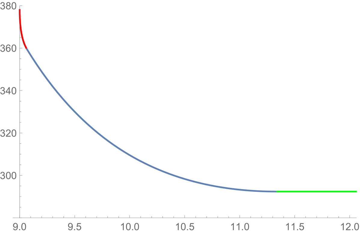
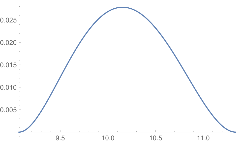
Theorem 3.4 is proven by solving of Theorem 3.2. In particular, the induced competitive ratio of for the choices of Theorem 3.4 is summarized in Figure 1 (Appendix A). Speed values , are chosen optimally when is either at most or at least (i.e. optimizers to admit analytic description). The optimal speed parameters when cannot be determined analytically (they are roots of high degree polynomials). The values that appear in Theorem 3.4 are heuristically chosen, but interestingly induce nearly optimal competitive ratio, see Figure 2 (Appendix A).
The proof of Theorem 3.4 is given by Lemma 3.6 (the case ), Lemma 3.7 (the case ), and Lemma 3.8 (the case ). Next we state these Lemmata, and we sketch their proofs.
Lemma 3.6 (Proof on page C.4).
For every , where , the optimizers to are , and . The induced competitive ratio is , (see definition of for in statement of Theorem 3.4), and the energy consumption, for instances , is .
For proving Lemma 3.6, first we recall the known optimizer for the special case (see Corollary C.6 within the Proof of Lemma 3.6 on page C.4), and we identify the tight constraints. Requiring that the exact same inequality constraints to remain tight, we ask how large can the product be so as to have KKT condition hold true. From the corresponding algebraic system, we obtain the answer .
Similarly, from Theorem 3.3 we know the optimizers to for large enough values of , and the corresponding tight constraints to the NLP. Again, using KKT conditions, we show that the same constraints remain tight for the optimizers as long as . This way we obtain the following Lemma.
Lemma 3.7 (Proof on page C.5).
For every , the optimal speeds of for are i.e. they are the same as for . If the target is placed at distance from the origin, then the induced energy equals . Moreover, the induced competitive ratio is , and is independent of .
The case can be solved optimally only numerically, since the best speed values are obtained by roots to a high degree polynomial. Nevertheless, the following lemma proposes a heuristic choice of speeds (that of Theorem 3.4) which is surprisingly close to the optimal (as suggested by Theorem 3.4, see also Figure 2).
Lemma 3.8 (Proof on page C.6).
The choices of of Theorem 3.4 when are feasible. Moreover, the induced competitive ratio is at most 0.03 additively off from the competitive ratio induced by the optimal choices of speeds (evaluated numerically).
The trick in order to find ``good enough'' optimizers to is to guess the subset of inequality constraints that remain tight when . First, we observe that constraint is tight for the provable optimizers for all when . As the only other constraint that switches from being tight to non-tight in the same interval is , we are motivated to maintain tightness for constraints and the time constraint. Still the algebraic system associated with the corresponding KKT conditions cannot be solved analytically. To bypass this difficulty, and assuming we know (optimal) speed , we use the tight time constraint to find speed as a function of . From numerical calculations, we see that optimal speed is nearly optimal in , and so we heuristically set . We choose so as to have satisfy optimality conditions for the boundary values . After we identify all parameters to our solution, we compare the value of our solution to the optimal one (obtained numerically), and we verify (using numerical calculations) that our heuristic solution is only by at most 0.03 additively off. The advantage of our analysis is that we obtain closed formulas for the speed parameters for all values of .
4 Solving with Unbounded-Memory Robots
In this section we prove Theorem 4.7, that is we solve by assuming that the two robots have unbounded memory, and in particular that they can perform time and state dependent calculations and tasks. Note that, by scaling, our results hold for all for which . For simplicity our exposition is for the natural case and . Also, as before, will denote the unknown distance of the exit from the origin, still the exit is assumed, for the purposes of performance analysis, to be at least 2 away from the origin.
Throughout the execution of our evacuation algorithm, robots can be in 3 different states (similar to the case of constant-memory robots). First, both robots start with the Exploration State and they remain in this until the exit is located. While in the exploration state, robots execute an elaborate exploration that requires synchronous movements in which robots, at a high level, stay in good proximity, still they expand the searched space relatively fast. Then, the exit finder enters the Chasing State in which the robot, depending on its distance from the origin, calculates a speed, at which to move in order to catch and notify the other robot. Lastly, when the two robots meet, they both enter the Exit State in which both robots move toward the exit with the smallest possible speed while meeting the time constraint.
Our algorithm takes as input the values of , and use a speed value , that will be chosen later. When the exit finder switches its state from Exploration to Chasing, it remembers the distance of the exit to the origin, as well as the value of a counter that was used while in the Exploration State. When the exit finder catches the other robot, they both switch to the Exit State, and they remember their distance from the origin, as well as the value of time that their rendezvous was realized. The speed of their Exit State will be determined as a function of (and hence of as well).
4.1 A Critical Component: -Phase Explorations
We adopt the language of [15] in order to discuss a structural property that any feasible evacuation algorithm for satisfies. As a result, the purpose of this section is to provide high level intuition for our evacuation algorithm that is presented in subsequent sections.
We refer to the two robots (starting exploration from the origin) as and , intended to explore to the left and to the right of the origin, respectively. The robot trajectories can be drawn on the Cartesian plane where point-location will correspond to point on the line being visited by some robot at time . The following Theorem is due to [15] and was originally phrased for the time-evacuation unit-speed robots' problem. We adopt the language of our problem.
Theorem 4.1.
For any feasible solution to , the point-location of any robot lies within the cone spanned by vectors .
Next we present some preliminaries toward describing our -phase exploration algorithms. A phase is a pair where is a speed and is a distance ratio, possibly negative. An -phase algorithm is determined by a position on the line and a sequence of phases (movement instructions). Whenever , movement will be to the left, whereas will correspond to movement to the right.
We will make sure that each time the loop is executed, position and corresponding time induce point-locations of the robots that lie in the boundary of the cone of Theorem 4.1. If a loop starts at location , then it takes additional time to complete one iteration. We will be referring to quantity as the expansion factor of Exploration .
4.2 Algorithm : The Exploration, Chasing and Exit States
In this section we give a formal description of our evacuation algorithm. The most elaborate part of it is when robots are in Exploration States, in which they will perform -phase exploration. It can be shown that -phase exploration based evacuation algorithms that do not violate the constraints of problem have expansion factor at most 4. Moreover, among those, the ones who minimize the induced energy consumption energy consumption make robots move at speed 1 in the first and third phase‡‡‡The proof of these facts is lengthy and technical, and is not required for the correctness of our algorithm, rather it only justifies some parameter choices. Robot's speed in the second phase will be denoted by .
We now present a specific -phase exploration algorithm, that we denote by , complying with the above conditions, with phases and , where is an exploration speed to be determined later. Robot will execute the 3-phase exploration with starting position -1, while robot with starting position . When subroutine is invoked, the robot sets its speed to and, from its current position, goes toward position on the line until it reaches it. We depict the trajectories of the robots while in the Exploration State in Figure 3.
Exploration State of repeat end Exploration State of repeat end
A complete execution of one repeat loop within the Exploration State will be referred to as a round. Variable counts the number of completed rounds. Each robot stays in the Exploration State till the exit it found. When switching to the Chasing state (which happens only for the exit finder), robot remembers its current value of counter , as well as the distance of the exit to the origin. Based on these values (as well as ) it calculates the most efficient trajectory in order to catch the other robot (predicting, when applicable, that the rendezvous can be realized while the other robot is approaching the exit finder). When the rendezvous is realized, robots store their current distance to the origin, as well as the time that has already passed. Then, robots need to travel distance to reach the exit. Knowing they have time remaining, they go to the exit together as slow as possible to reach the exit in time exactly . Figure 4 provides an illustration of the behavior of the robots after finding the exit.
Chasing State if I am then end if Travel toward the other robot at speed until meeting it at distance from the origin, and at time . Exit State Go toward the exit with speed .
4.3 Performance Analysis & an Optimal Choice for Parameter
In this section we are ready to provide the details for proving Theorem 4.7. Evacuation algorithm is not feasible to for all values of speed parameter (of the Exploration States). We will show later that trajectories induce evacuation time at most only if . In what follows, and even though we have not fixed the value of yet, we will assume that has some value between 1/3 and 1/2. The purpose of this section is to fix a value for parameter , show that is feasible to , and subsequently compute the induced energy consumption and competitive ratio. As a reminder, each iteration of the repeat loop of the Exploration States is called a round, and is a counter for these rounds.
Proposition 4.2 (Proof on page D.1).
For every , and at the start of its -th round,
robot is at position at time , and
robot , is at position at time .
Let be one of the robots. We define if , and if , i.e. the position of at the start of round . We will often analyze 3 cases for the distance of the exit with respect to (as it also appears in the description of the Chasing State), associated with the following closed intervals
We may simply write and if is clear from the context. Note that during the second phase of round , robot explores and , whereas is explored during the third phase. The same statement holds for . The following lemma will be useful in analyzing the worst case evacuation time and energy consumption of our algorithm.
Lemma 4.3 (Proof on page D.2).
Suppose that robot finds the exit at distance when its round counter has value . Let and be, respectively, the position and time at which first meets with the other robot after having found the exit, and set . Then the following hold:
-
1.
If , then and .
-
2.
If , then and .
-
3.
If , then and .
Using the lemma above, we can now prove that meets the speed bound and the evacuation time bound.
Lemma 4.4 (Proof on page D.3).
For any , evacuation algorithm is feasible to .
Lemma 4.3 allows us to derive the speed and at which both robots go toward the exit after meeting for the cases and , respectively. We also know the speed at which the exit-finder catches up to the other robot when . We define
The speed is a simple rearrangement of the speed , and is obtained by rearranging .
Next compute the energy consumption. For given and , denote by the energy spent by robot from time to time when it exits. Similarly, is the energy spent by from time to time . Then, then energy consumption is . For any and , we also define .
Lemma 4.5 (Proof on page D.4).
Suppose that robot finds the exit at distance when its round counter has value , and let . Then
Denote by the value of when , . Our intension now is to fix speed value that solves the following Nonlinear Program
For every we show in Lemma 4.6 that is decreasing in , that is increasing in , and that is decreasing in . Then, the best parameter can be chosen so as to make all worst case valued equal (if possible) when . The optimal can be found by numerically finding the roots of a high degree polynomial, and accordingly, we heuristically set , inducing the best possible energy consumption for algorithm . All relevant formal arguments are within the proof of the next lemma.
Lemma 4.6 (Proof on Page D.5).
On instance of , algorithm induces energy consumption at most , when .
By Lemma 4.6, we conclude that for the specific value of , algorithm has competitive ratio concluding the proof of Theorem 4.7.
Theorem 4.7.
For every with , there is an evacuation algorithm for unbounded-memory autonomous robots solving inducing energy consumption for instances , and competitive ratio 341.24814.
Acknowledgements
Research supported by NSERC discovery grants, NSERC graduate scholarship, and NSF.
References
- [1] S. Alpern and S. Gal. The theory of search games and rendezvous. Springer, 2003.
- [2] R. Baeza Yates, J. Culberson, and G. Rawlins. Searching in the plane. Information and Computation, 106(2):234–252, 1993.
- [3] R. Baeza-Yates and R. Schott. Parallel searching in the plane. Computational Geometry, 5(3):143–154, 1995.
- [4] E. Bampas, J. Czyzowicz, L. Gasieniec, D. Ilcinkas, R. Klasing, T. Kociumaka, and D. Pajak. Linear search by a pair of distinct-speed robots. Algorithmica, 81(1):317–342, 2019.
- [5] G. K. Batchelor. An Introduction to Fluid Dynamics. Cambridge Mathematical Library. Cambridge University Press, 2000.
- [6] A. Beck. On the linear search problem. Israel J. of Mathematics, 2(4):221–228, 1964.
- [7] R. Bellman. An optimal search. SIAM Review, 5(3):274–274, 1963.
- [8] M. Blum and D. Kozen. On the power of the compass (or, why mazes are easier to search than graphs). In FOCS, pages 132–142, 1978.
- [9] P. Bose and J.-L. De Carufel. A general framework for searching on a line. Theoretical Computer Science, pages 703:1–17, 2017.
- [10] P. Bose, J.-L. De Carufel, and S. Durocher. Searching on a line: A complete characterization of the optimal solution. Theoretical Computer Science, pages 569:24–42, 2015.
- [11] S. Brandt, K.-T. Foerster, B. Richner, and R. Wattenhofer. Wireless evacuation on m rays with k searchers. In SIROCCO, pages 140–157, 2017.
- [12] S. Brandt, F. Laufenberg, Y. Lv, D. Stolz, and R. Wattenhofer. Collaboration without communication: Evacuating two robots from a disk. In CIAC, pages 104–115, 2017.
- [13] S. Brandt, J. Uitto, and R. Wattenhofer. A tight lower bound for semi-synchronous collaborative grid exploration. In DISC, pages 13:1–13:17, 2018.
- [14] L. Budach. Automata and labyrinths. Math. Nachrichten, 86:195–282, 1978.
- [15] M. Chrobak, L. Gasieniec, Gorry T., and R. Martin. Group search on the line. In SOFSEM, pages 164–176. Springer, 2015.
- [16] H. Chuangpishit, K. Georgiou, and P. Sharma. Average case - worst case tradeoffs for evacuating 2 robots from the disk in the face-to-face model. In ALGOSENSORS'18. Springer, 2018.
- [17] S. A. Cook and C. Rackoff. Space lower bounds for maze threadability on restricted machines. SIAM Journal on Computing, 9(3):636–652, 1980.
- [18] J. Czyzowicz, L. Gasieniec, T. Gorry, E. Kranakis, R. Martin, and D. Pajak. Evacuating robots via unknown exit in a disk. In DISC, pages 122–136. Springer, 2014.
- [19] J. Czyzowicz, K. Georgiou, R. Killick, E. Kranakis, D. Krizanc, L. Narayanan, J. Opatrny, and S. Shende. God save the queen. In (FUN), pages 16:1–16:20, 2018.
- [20] J. Czyzowicz, K. Georgiou, R. Killick, E. Kranakis, D. Krizanc, L. Narayanan, J. Opatrny, and S. Shende. Priority evacuation from a disk using mobile robots. In SIROCCO, pages 209–225, 2018.
- [21] J. Czyzowicz, K. Georgiou, and E. Kranakis. Group search and Evacuation. In Distributed Computing by Mobile Entities, Current Research in Moving and Computing, LNCS, volume 11340, pages 335–370, 2019.
- [22] J. Czyzowicz, K. Georgiou, E. Kranakis, D. Krizanc, L. Narayanan, J. Opatrny, and S. Shende. Search on a line by byzantine robots. In ISAAC, pages 27:1–27:12, 2016.
- [23] J. Czyzowicz, K. Georgiou, E. Kranakis, L. Narayanan, J. Opatrny, and B. Vogtenhuber. Evacuating robots from a disc using face to face communication. In CIAC 2015, pages 140–152, 2015.
- [24] J. Czyzowicz, E. Kranakis, D. Krizanc, L. Narayanan, and Opatrny J. Search on a line with faulty robots. In PODC, pages 405–414. ACM, 2016.
- [25] J. Czyzowicz, E. Kranakis, D. Krizanc, L. Narayanan, J. Opatrny, and M. Shende. Linear search with terrain-dependent speeds. In CIAC, pages 430–441, 2017.
- [26] J. Czyzowicz, E. Kranakis, K. Krizanc, L. Narayanan, J. Opatrny, and S. Shende. Wireless autonomous robot evacuation from equilateral triangles and squares. In ADHOCNOW, pages 181–194. Springer, 2015.
- [27] E. D. Demaine, S. P. Fekete, and S. Gal. Online searching with turn cost. Theoretical Computer Science, 361(2):342–355, 2006.
- [28] Y. Emek, T. Langner, D. Stolz, J. Uitto, and R. Wattenhofer. How many ants does it take to find the food? Theor. Comput. Sci., page 608:255–267, 2015.
- [29] S. Gal. Search Games. Wiley Encyclopedia for Operations Research and Management Science, 2011.
- [30] K. Georgiou, G. Karakostas, and E. Kranakis. Search-and-fetch with one robot on a disk - (track: Wireless and geometry). In ALGOSENSORS, pages 80–94, 2016.
- [31] K. Georgiou, G. Karakostas, and E. Kranakis. Search-and-fetch with 2 robots on a disk - wireless and face-to-face communication models. In ICORES, pages 15–26. SciTePress, 2017.
- [32] F. Hoffmann, C. Icking, R. Klein, and K. Kriegel. The polygon exploration problem. SIAM Journal on Computing, 31(2):577–600, 2001.
- [33] M.-Y. Kao, J. H. Reif, and S. R. Tate. Searching in an unknown environment: An optimal randomized algorithm for the cow-path problem. Information and Computation, 131(1):63–79, 1996.
- [34] J. Kleinberg. On-line search in a simple polygon. In SODA, pages 8–15. SIAM, 1994.
- [35] I. Lamprou, R. Martin, and S. Schewe. Fast two-robot disk evacuation with wireless communication. In DISC, pages 1–15, 2016.
- [36] D. Pattanayak, H. Ramesh, P.S. Mandal, and S. Schmid. Evacuating two robots from two unknown exits on the perimeter of a disk with wireless communication. In ICDCN, pages 20:1–20:4, 2018.
- [37] O. Reingold. Undirected st-connectivity in log-space. In STOC, pages 376–385, 2005.
- [38] H.-A. Rollik. Automaten in planaren graphen. Acta Informatica, 13(3):287– 298, 1980.
Appendix A Figures


Appendix B Observation B.1
Observation B.1.
is well defined for each with , and the optimal solution, given that instance is known, equals .
Proof: [Proof of Observation B.1] Given that the location of the exit is known, and by symmetry, it is immediate that both robots have the same optimal speed, call it , and they move in the direction of the exit. The induced evacuation time is then , and the induced evacuation energy is . For a feasible solution we require that and that , and hence, the optimal offline solution is obtained as the solution to For a feasible solution to exist, we need . Moreover, it is immediate that the optimal choice is , inducing energy consumption . ∎
Appendix C Proofs Omitted from Section 3.
C.1 Lemma 3.1
Proof: [Proof of Lemma 3.1] Consider the moment that the exit is located, after time time of searching. The robot that now chases the other speed- robot at constant speed will reach it after time. To see this note that the configuration is equivalent to that the speed- robot is immobile and the other robot moves at speed , having to traverse a total distance of . Moreover, the speed- robot traverses an additional length segment till it is caught, being a total of away from the exit. Once robots meet, the walk to the exit at speed , which takes additional time . Overall the evacuation time equals
Similarly we compute the total energy till both robots reach the exit. The energy spent by the finder is
while the energy spent by the non finder is
Adding the two quantities and simplifying gives the promised formula. ∎
C.2 Theorem 3.2
Proof: [Proof of Theorem 3.2] Note that in that aims to provide a solution to , constraints are simply omitted. In particular, the theorem above claims that when , i.e. when speeds are unbounded, algorithm always admits some feasible solution. In what follows, we prove all claims of the theorem.
By Lemma 3.1, the energy performance of equals , and the induced evacuation time is . For the values of to be feasible, we need that , that and that . Clearly the latter time constraint simplifies to the time constraint of , while the objective value can be scaled by without affecting the optimizers to the NLP, if such optimizers exist. Finally note that even though the strict inequalities become non strict inequalities in the NLP, speeds evaluations for which any of is 0 or violates the time constraint (for any fixed ). Therefore, correctly formulates the problem of choosing optimal values for for solving .
The next two lemmas show that the Naive algorithm can solve problem for the entire spectrum of values for which the problem admits solutions, as per Lemma 2.1.
Lemma C.1.
For every , problem admits an optimal solution.
Proof: [Proof of Lemma C.1] Consider the redundant constraints that can be derived by the existing constraints of (note that if all speeds are not at least then clearly the time constraint is violated). For the same reason, it is also easy to see that , since again we would have a violation of the time constraint.
Next, it is easy to check that is a feasible solution, hence the NLP is not infeasible. The value of the objective for this evaluation is . But then, notice that the objective is bounded from below by . Hence, if an optimal solution exists, constraints are valid for the optimizers. We may add these constraints to , resulting into a compact (closed and bounded) feasible region. But then, note that the objective is continuous over the new compact feasible region, hence from the extreme value theorem it attains a minimum. ∎
Lemma C.2.
There exist for which induces a feasible solution to if and only if .
Proof: [Proof of Lemma C.2] Consider the problem of minimizing completion time of the Naive Algorithm, given that the speeds are all bounded above by . The corresponding NLP that solves the problem reads as.
| (2) | ||||
Note that it is enough to prove that the optimal value to (2) is . Indeed, that would imply that no speeds exist that induce completion time less than , making the corresponding feasible region of empty if .
Now we show that the optimal value to (2) is , by showing that the unique optimizers to the NLP are and . Indeed, note that
which is strictly negative for all feasible with . Hence, there is no optimal solution for which , as otherwise by increasing one could improve the value of the objective. Similarly we observe that
which is again strictly negative for all feasible with . Hence, there is no optimal solution for which , as otherwise by increasing one could improve the value of the objective.
To conclude, in an optimal solution to (2) we have that , and hence one needs to find minimizing . For this we compute
and it is easy to see that if and only if or (and the latter is infeasible). At the same time, is convex when because , hence corresponds to the unique minimizer. ∎
The last component of Theorem 3.2 that requires justification pertains to the competitive ratio. Now fix for which , and let be the optimal solution to (corresponding to the optimal choices of algorithm ). By Lemma 3.1 the induced energy consumption is . Then, the competitive ratio of the algorithm is ∎
C.3 Theorem 3.3
Proof: [Proof of Theorem 3.3] First we observe that are indeed feasible to (for every ), since
and in particular, for the values of described above we have (from the formal definition of that appears later, it will be clear that expression will be exactly equal to 1). Moreover, by Theorem 3.2, the competitive ratio of is
as claimed.
In the remaining of the section we prove that the choices for of Theorem 3.3 are indeed optimal for . First we establish a structural property of optimal speeds choices for .
Lemma C.3.
For any , optimal solutions to satisfy constraint tightly.
Proof: Consider an optimal solution . As noted before, we must have and , as otherwise the values would be infeasible.
Next note that the time constraint can be rewritten as
For the sake of contradiction, assume that the time constraint is not tight for . Then, there is so that is a feasible solution, where . But then, the objective value strictly decreases, a contradiction to optimality. ∎
We will soon derive the optimizers to using Karush-Kuhn-Tucker (KKT) conditions. Before that, we observe that solutions are scalable with respect to , which will also allow us to simplify our calculations.
Lemma C.4.
Let be the optimizers to inducing optimal energy . Then, for any , the optimizers to are , and the induced optimal energy is .
Proof: Note that the triplet is feasible to (for a specific ) if and only if the triplet is feasible to . Moreover, it is straightforward that when speeds are scaled by , the induced energy is scaled by . Hence, for every there is a bijection between feasible (and optimal) solutions to and . ∎
We are therefore motivated to solve , and that will allow us to derive the optimizers for , for any .
Lemma C.5.
The optimal solution to is obtained for
and the optimal NLP value is .
Proof: By KKT conditions, we know that, necessarily, all minimizers of satisfy the condition that is a conical combination of tight constraints (for the optimizers). Lemma C.3 asserts that has to be satisfied for all optimizers . At the same time, recall that, by the proof of Lemma C.1, none of the constraints and can be tight for an optimizer. Hence, KKT conditions imply that any optimizer satisfies, necessarily, the following system of nonlinear constraints
More explicitly, the first equality constraints is
From the 3rd coordinates of the gradients, we obtain that , which directly implies that the dual multiplier preserves the correct sign for the necessary optimality conditions.
Hence, the original system of nonlinear constraints is equivalent to that
Using software numerical methods, we see that the above algebraic system admits the following 3 real roots for :
Since also all speeds are nonnegative, we obtain the unique candidate optimizer
To verify that indeed is a minimizer, we compute
Moreover,
which has eigenvalues , hence it is PSD. As a result, is locally convex at , and therefore is a local minimizer to . As we showed earlier, is the only candidate optimizer, hence a global minimizer as well.
∎
C.4 Lemma 3.6
Proof: [Proof of Lemma 3.6]
An immediate corollary from the proof of Lemma C.2 (within the proof of Theorem 3.2) is the following
Corollary C.6.
The unique solution to when is given by
inducing energy , and competitive ratio .
Next we find solutions for so that remain tight. Since, when , there is only one optimizer , two inequality constraints are tight. The next calculations investigate the spectrum of for which the same constraints remain tight for the optimizer.
We write 1st order necessary optimality conditions for , given that the candidate optimizer satisfies the time constraint, and the two speed bound constraints tightly
From the tight time constraint, and solving for we obtain that
For each , the first gradient equality defines a linear system over whose solutions are
respectively. As long as all dual multiplies are positive, corresponding solution is optimal to , provided that .
First we claim that cannot be part of an optimizer. Indeed,
Recall that , and hence the denominator of as well as are strictly positive. But then, the sign of is exactly the opposite of . Define function over the domain . It is easy to verify that preserves positive sign (in fact Hence, that concludes our claim.
Next we investigate the spectrum of for which all remain non-negative.
Our next claim is that for all we have that . Indeed, consider function
It is easy to see that . But then, elementary calculations show that , proving that as claimed.
Next we investigate the sign of . For this, introduce function , and note that
Claim 1: for all .
Define and . Note that .
Simple calculus shows that is strictly decreasing in , and , and therefore for all . Similarly, it is easy to see that is strictly increasing in , and . Therefore for all . Overall this implies that is positive for all .
Claim 2: for all .
First we observe that the denominator of preserves positive sign for . So we focus on the sign of the numerator we we abbreviate by
.
Note that is equivalent to that
Degree-3 polynomial has only one real root, which is
Hence, for all
Claim 3: for all .
First we observe that the denominator of preserves positive sign for . So we focus on the sign of the numerator we we abbreviate by
.
Note that is equivalent to that
The roots of degree-3 polynomial are
We conclude that preserves positive sign for all .
Overall, we have shown that feasible solution satisfies necessary 1st order optimality conditions. We proceed by checking that satisfy 2nd order sufficient conditions, which amounts to showing that . Indeed,
By setting , we obtain the simpler form
| (3) |
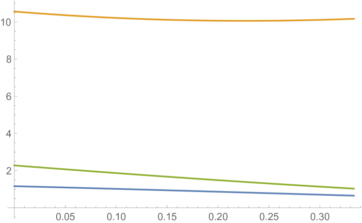
When we have that , is decreasing in the product of , and it remains positive. The eigenvalues of the matrix that depends only on and for any can be obtained using a closed formula (they are real roots of a degree-3 polynomial). In Figure 5 we depict their behavior. Since all eigenvalues are all positive, the candidate optimizer is indeed a minimizer.
∎
C.5 Lemma 3.7
C.6 Lemma 3.8
Proof: [Proof of Lemma 3.8] First, we observe that constraint is tight for the provable optimizers for all when . As the only other constraint that switches from being tight to non-tight in the same interval is , we are motivated to maintain tightness for constraints and the time constraint.
Given that speed is chosen (to be determined later), we fix , and we set where
so as to satisfy the time constraint tightly (by solving for ). It remains to determine values for speed . To this end, we heuristically require that where
for some constants that we allow to depend on . In what follows we abbreviate by . Let be the chosen values for speed as summarized by the statement of Theorem 3.4 when and , respectively. We require that
inducing a linear system on . By solving the linear system, we obtain
Using the known values for , we obtain , as promised. It remains to argue that , together with , and are feasible when .
The fact that complies with bounds follows immediately, since is a linear strictly decreasing function in , and both satisfy the bounds by construction. We are therefore left with checking that which is equivalent to that
Define degree-2 polynomial function and observe that it sufficies to prove that for all . The roots of can be numerically computed as , proving that preserves positive sign in as wanted.
Finally, the claims regarding the induced energy and competitive ratio is implied by Theorem 3.2 and obtained by evaluating the given choices of in . ∎
Appendix D Proofs Omitted from Section 4.
D.1 Proposition 4.2
Proof: [Proof of Proposition 4.2] The exploration algorithm explicitly ensures that round ends (and hence that round begins) at the claimed position, so only the time needs to be proved. Note that the statement is true for both robots when . Suppose that when starts its -th round, it is at position at time . The round ends at time , and the -th round will start at the claimed time. The proof is identical for . ∎
D.2 Lemma 4.3
Proof: [Proof of Lemma 4.3] Case 1: . Let be the robot other than . Observe that by Proposition 4.2, finds the exit at time . Then goes towards at speed , and so it will reach position at time . We know that at time , robot is starting a round at position or , then goes towards at full speed. Hence is at position at time , where it meets .
Case 2: . As before, the exit is found at time . Assume for simplicity that (the case is identical by symmetry). After finding the exit at position , goes full speed to the right. Thus at time , it arrives at position . We show that at this time, is in its second phase and is at this position. Notice that
the latter inequality being obtained from . Now, enters its second phase when at position at time , and the phase ends a time . Since , we get . Therefore is still in its second phase at time , and it follows that its position at this time is . Hence and meet. It is straightforward to see that and could not have met before time , and thus and meet at the claimed time and position. Case 3: . Again assume that . This time finds the exit at position at time . Going full speed to the right, at time , it reaches position . Since , we have . As in the previous case, the second phase of ends at time . Thus at time , is at position . Again, one can check that and could not have met before, which concludes the proof. ∎
D.3 Lemma 4.4
Proof: [Proof of Lemma 4.4] Let be the robot that finds the exit at distance , and let . We show that all speeds are at most 1, as well as that the evacuation time is at most . There are three cases to consider.
Case 1: . By Lemma 4.3, after meeting, both robots need to travel distance and have time remaining. By the last line of the exit phase algorithm, they go back at speed and make it in time, provided that speed is achievable, i.e. . Clearly since . If we assume , we get , leading to , a contradiction.
Case 2: . By Lemma 4.3, the robots meet at position such that at time . The robots use the smallest speed that allows the them to reach the exit in time . We must check that . We argue that if the two robots used speed to get to the exit after meeting, they would make it before time . Since allows the robots to reach the exit in time exactly , it follows that .
First note that since , we have . Using speed from the point they meet, the robots would reach the exit at time
where we have used the fact that in the inequality. It is straighforward to show that when , proving our claim.
Case 3: . Again according to Lemma 4.3, the robots meet at position satisfying at time . The robots go towards the exit at speed . As in the previous case, we show that is a valid speed by arguing that the robots have enough time if they used their full speed. If they do use speed after they meet, they reach the exit at time . Since , we have . Therefore . One can check that this is or less whenever . ∎
D.4 Lemma 4.5
Proof: [Proof of Lemma 4.5] For any power of with , define as the energy spent by after reaching position for the first time without having found the exit, ignoring the initial energy spent to get to position . The quantity is the sum of energy spent in each of the first rounds, and so
We define similarly for , i.e. is the energy spent by when its -th round is finished and it reached position for the first time, ignoring the initial energy to get at position . We get
We may now calculate the three possible cases of energy. Assume that finds the exit and . Observe that
We implictly use Lemma 4.3 for the distance traveled by to catch up to after finding the exit, and the distance traveled back by both robots. In the expressions that follow, for clarity we partition the terms into 3 brackets, which respectively represent the energy spent by to find the exit and catch up to , the energy spent by before being caught, and the energy spent by both robots to go to the exit.
Case 1: . The total energy spent is
Case 2: . In this case, the energy spent is
Case 3: . The energy spent is
∎
D.5 Lemma 4.6
Proof: [Proof of Lemma 4.6] We analyze each case separately.
Case 1: . According to Lemma 4.5, we have
Consider the case . Plugging in , the above evaluates to . We claim that is a decreasing function over interval , and therefore attains its maximum when . Assuming this is true, adding the initialization energy of omitted so far and given that , the energy ratio is at most
We now prove that is decreasing over the interval . Let
and observe that
The plan is to prove that
For this we calculate
Now we claim that all are increasing functions in , for . Indeed, first,
since . Hence is increasing in .
Second,
is positive (and well defined), since . Hence is increasing in .
Third, we show that is increasing in . For this it is enough to prove that For (and in fact for all ) the strict inequality can be written as which we show next it is satisfied. Indeed, it is easy to see that (which is attained for ), while , hence the claim follows.
To resume, we showed that are increasing functions in , for . Recalling that , and since , we obtain that
Since , the latter quantity is clearly negative. This shows that is negative (in the given domain), hence is decreasing in .
Case 2: . In this case, the energy ratio is
We will show that this expression achieves its maximum at . When , then above yields . Given that , this implies that the energy ratio is at most
We prove that is an increasing function over interval . First we compute and we substitute to find , where
Note that , and hence for all values of under consideration. Therefore the lemma will follow if we show that as well.
is a degree-3 polynomial with positive leading coefficient. It attains a local minimum at the largest real root of
which is
Now we observe that for all , we have .
From the above, it follows that is monotonically increasing for , and therefore
as wanted.
Case 3: . The energy ratio is
In this case, we claim that this expression is decreasing over and achieves its maximum at . When , the above gives (which is the same as in case 2, as one should expect). Given that , we get that the energy ratio is at most
Let us prove that is indeed decreasing. Note that equals
where
In what follows we prove that both are strictly decreasing when , implying the claim of the lemma.
First we show that is decreasing. For that note that, using the fixed value of , we have , and the latter expression (in ) is clearly strictly decreasing for all constants .
Now we show that is strictly decreasing for all . For that observe that for the specific constant , and since , we have that
Hence, to show that is strictly decreasing, it is enough to prove that
is strictly decreasing in . First observe that the rational function is well defined for these values of , since the denominator becomes 0 only when (the last inequality is easy to verify). To that end, we compute
which is of course negative for the given value of .
∎