Energy measures of harmonic functions on the Sierpiński Gasket
Abstract.
We study energy measures on SG based on harmonic functions. We characterize the positive energy measures through studying the bounds of Radon-Nikodym derivatives with respect to the Kusuoka measure. We prove a limited continuity of the derivative on the graph and express the average value of the derivative on a whole cell as a weighted average of the values on the boundary vertices. We also prove some characterizations and properties of the weights.
Key words and phrases:
Sierpiński gasket, energy measures, Kusuoka measure, energy Laplacian, Radon-Nikodym derivatives2010 Mathematics Subject Classification:
28A801. introduction
In the development of analysis on fractals, there are three basic concepts: energy, measure and Laplacian. For , which may be regarded as the “poster child” for the theory, Kigami has developed an elegant construction of a self-similar Laplacian based on a self-similar energy and self-similar measure via an analog of integration by parts. This theory is briefly sketched below, and is described in complete detail in the book [8]. This standard Laplacian is not the only Laplacian on that has been widely studied. A competing energy Laplacian , based on the same energy but using the Kusuoka measure in place of , has received a lot of attention in recent years([4, 5, 6, 10, 11]). It has two striking advantages over , namely the existence of a Leibniz-type product formula and the fact that the associated heat kernel satisfies Gaussian type estimates. The main drawback so far has been that the Kusuoka measure is not algorithmically transparent. The purpose of this paper is to eliminate this drawback. We will provide algorithms that describe the nature of this measure and more generally the family of energy measures based on harmonic functions , and the Radon-Nikodym derivatives . Some of the results of this paper, especially Theorem 5.5, may also be derived from [6].
The Sierpiński gasket, or simply SG, is the unique nonempty compact set satisfying
where and are vertices of an equilateral triangle in counter-clockwise direction. are called the boundary points of SG. If is a finite word, we define the mapping where is defined to be the length of the word. Define , and . For the boundary of a cell , denoted by , we mean the three vertices of the cell.
For functions , defined on SG, we define the energy on level by
| (1.1) |
and energy provided that and are finite. For each cell , we define the energy of , on this cell by
Observe that the energy is non-negative if , but in general it is not. In the case , we write instead of . We define a function to be harmonic if it minimizes the energy from level to level , as defined in (1.1). A simple computation shows that this minimization occurs when at which to each cell , . Equivalently, a function on SG is harmonic if the sequence, taking in (1.1), is a constant sequence, i.e. constantly . Given three values on the boundary, in order to have a constant sequence in (1.1), all the other values are completely determined. Consequently, all the harmonic functions form a three-dimensional space and hence any values on the boundary of a cell can extend to a unique harmonic function on SG. A harmonic function is said to be symmetric(resp. skew-symmetric) if (resp. ) for some . Harmonic functions characterized by are three symmetric functions and the notation will be used throughout this paper. On the space of harmonic functions modulo constants, ) is a two-dimensional inner product space. A harmonic function is said to be symmetric (resp. skew-symmetric) in if there exists a constant and a symmetric (resp. skew-symmetric) harmonic function such that . Explicitly, for a symmetric harmonic function , we mean for some and some ; and for a skew-symmetric harmonic function , we mean for some and . To each harmonic , we write the harmonic function having the same energy as and orthogonal to unless we specify “orthonormal to ” in which case we mean having energy and orthogonal to .
The standard measure is a self-similar measure characterized by for every cell . The standard Laplacian of is a continuous function satisfying
| (1.2) |
for every vanishing at the boundary with . Harmonic functions on SG are precisely those whose Laplacian is zero. However, for a function whenever is defined as a function, is not defined as a function. We can view as a measure and exists as a function if and only if this measure is absolutely continuous with respect to the standard measure. The carré du champs formula given by, for all of finite energy, shows that
for all with as a function. Thus if exists as a function and if we first view as a measure,
then would exist as a function if this measure were absolutely continuous with respect to the standard measure , but this is almost never the case [2].
Suppose that , are functions of finite energy. We can define a signed measure by, on each cell,
As usual, if it happens that , we write instead. In this paper, we will restrict the attention to both , being harmonic. The energy measures of harmonic functions form a three-dimensional space. The Kusuoka measure is defined to be . An easy computation shows that for any harmonic function , we have where . Now, we define the energy Laplacian of by, for every finite energy vanishing on the boundary,
| (1.3) |
By Theorem 5.3.1 of [8], every energy measure of harmonic functions is absolutely continuous with respect to the Kusuoka measure and it makes sense to consider the Radon-Nikodym derivatives. For the energy measures of the symmetric harmonic functions, we will denote these by instead of . forms a basis of the space of all energy measures of harmonic functions. Since , we have for . Since for all , , this gives us three equations that we solve to obtain
| (1.4) |
We will keep using the notation for any energy measure of harmonic functions without mentioning and .
By [1], we have that there exist matrices such that for every cell ,
The ’s are all diagonalizable, so it is easy to calculate . Explicitly, after diagonalization, we have
| (1.5) |
It is easy to calculate that the limits of quotients which are used to compute derivatives are as follows:
where
For each infinite word , let be the word consisting of the first letters of ; then . It follows that every energy measure is continuous.
It is natural to ask whether the energy Laplacian behaves in a similar manner to the standard Laplacian; in Section 2, we express the “self-similarity” of the energy Laplacian. In Section 3, we will study the decay rates of energy measure from a cell to its subcells. Through studying this, we give sharp bounds for the Radon-Nikodym derivatives for each . Being in general a signed measure, it is natural to ask when it is a (positive) measure; in Section 4, we will characterize all the positive energy measures. It is well-known that the derivative is not continuous; nevertheless, in Section 5, we show that a certain restriction of the derivative is continuous. In Section 6, we will express, on each cell, the average value of derivatives by a weighted average of values on vertices of the cell. How the energy distributes is mysterious; in Section 7, we will provide some graphs and hypothesis about this question.
2. Self-similarity of energy Laplacian
In this section we discuss the self-similarity identities for energy measures and the energy Laplacian. We will see that the Radon-Nikodym derivatives play a crucial role in these identities. Individually, none of the is self-similar; nevertheless, together they form a self-similar family, in the sense of Mauldin-Williams [7]. We begin with considering the symmetric function . We have the following equalities,
| (2.1) |
Next we establish the relation of ’s from cells to subcells.
Theorem 2.1.
Let
then
for every cell C. In other words,
Proof.
Corollary 2.2.
The Kusuoka measure satisfies the variable weight self-similar identity
| (2.2) |
Proof.
If we consider , where , the Radon-Nikodym Derivative of w.r.t. , we get
| (2.3) |
∎
We now give the “self-similarity” of the energy Laplacian .
Theorem 2.3.
Let . Then the energy Laplacian satisfies
Proof.
By the definition of the energy Laplacian and by (2.2),
On the other hand, the self-similarity of also gives
Together we have
Since is arbitary, and so is arbitary, we must have the self-similarity of
∎
Corollary 2.4.
Let be a finite word of length and . Define
Then
Proof.
Use the theorem and iterate. ∎
To compute on the cell , zoom in by looking at as a function on , compute its Laplacian and multiply by ,
and then zoom out via
3. Bounds of derivatives
By the definition of energy measures, we see that every energy measure is continuous; by the self similarity of SG, we see that it makes sense to consider the measure from cells to subcells. It is natural to study how the measure varies for a sequence of cells converging to a point.
Lemma 3.1.
For a harmonic function , if we let , , , then with equality if and only if is skew symmetric (with respect to ) on the cell .
Proof.
WLOG, let , , . Then, writing and a direct computation on the energies on each cell,
so and . Equality holds iff , in which case is skew symmetric. ∎
Lemma 3.2.
Let be a word. For
we have
Proof.
Since , we have by symmetry for . Thus
Now Lemma 3.1 implies for all , so adding these up yields . To complete the proof, we show that for some . Suppose, on the contrary, that each is skew symmetric with respect to on the cell . Then there exist such that , but this shows lie in a two-dimensional subspace, contradicting being linearly independent. ∎
Lemma 3.3.
For the sequence , which converges to the point , we have that , (here means and ).
Proof.
We prove this statement for ; the other cases are similar.
We know that
Now we let
and see from the diagonalization of that
since by Lemma 3.2. ∎
We have proven the decay rates of the measures of a sequence of cells converging to a point which is not equivalent to a skew-symmetric cell. Surprisingly, in the case which the cell is equivalent to skew-symmetric at that point, we have the first condition for the Radon-Nikodym derivatives to be .
Lemma 3.4.
If is symmetric on the cell with respect to the point , then and hence . Conversely, if , then is symmetric on the cell with respect to the point .
Proof.
We know that , so we may consider the case when is the empty word. We see from Lemmas 3.1 and 3.3 that the term in vanishes if and only if is skew-symmetric on with respect to the point , which is true if and only if is symmetric on with respect to the point , in which case and the denominator of dominates. It follows that symmetry of around is sufficient and necessary to have . ∎
Theorem 3.5.
Let be a harmonic function on SG with and be a harmonic function orthonormal to under the energy inner product. Also let be a cell in . Then
a)
b)
and if the maximum of is attained, then the minimum of is attained at the same point.
Proof.
We first prove a). If two of the values of on the boundary of are the same then is symmetric and the result follows from Lemma 3.4, so we assume all three values are distinct. Since we consider modulo constants and the conclusion is unchanged by replacing with a constant multiple , we may assume without loss of generality that is harmonic with , , . Let be the point on the edge from to where achieves its maximum. It was shown in [3] that if we identify this edge in the obvious fashion with the unit interval oriented so corresponds to and to , and define a map by , then is continuous and strictly decreasing, and that gives the midpoint . It follows that if we have a harmonic function on a cell such that the maximum along a side occurs at the midpoint of that side then the function is symmetric under the reflection fixing the vertex opposite the side. This is applicable in the case when the location of our maximum is (equivalently a dyadic point of under our identification), because then there is a word such that , and the function is harmonic on with its maximum along at the midpoint of this side. The conclusion that is symmetric on allows us to apply Lemma 3.4 to deduce that .
Now suppose that is not a dyadic point. Since dyadic points are dense in the interval [0,1], we pick a increasing sequence of dyadic points converging to . Because is decreasing and continuous, there exists a decreasing sequence of converging to satisfying .
Let be given. A simple computation shows that the energy measure . From the previous discussion, we can pick an (, resp.), which will be denoted as (, resp.), satisfying . We also denote the harmonic function with boundary values as . The previous discussion shows that . Now,
where the penultimate inequality comes from the fact that since for any cell .
And consequently,
On a general cell , is harmonic, so the same argument applies.
We then show b). An easy computation shows , where . Since the total measure of on is , we have
It follows that
Whence,
Further, if the derivative attains its supremum, then the maximum occurs where occurs in , that is, where the local extremum occurs in the smallest edge of the harmonic function . ∎
As we can see, on every cell of SG, the supremum and infimum are distance from each other, so the derivative is far from continuous. However, we will later recover limited continuity when we restrict to the edges of cells.
4. Characterzation of Positive Energy Measures
Within the 3-dimensional space of signed energy measures which measures are positive? The following result gives the answer.
Theorem 4.1.
Let be the set of such that is a positive energy measure. Then is the solid cone , and the boundary of is the set of such that for some harmonic function .
Proof.
We first show that . We know from [1] that the set of such that form the cone
A simple computation shows that
transforms to the corresponding coefficients . Hence, the set of that corresponds to some is the cone
which is the boundary of . Then a general point in has the form with all , so it yields a positive measure and so belongs to .
Now we show that the coefficients that come from harmonic functions (the boundary of ) are on the boundary of . Consider the energy measure for . Suppose, for contradiction, that this measure is positive. Then for any cell , , so for all , but we know the infimum should be zero, so this is a contradiction. Therefore and is on the boundary of . Since the two boundaries coincide, . ∎
Immediately, since the solid cone is convex, every positive energy measure is precisely a convex combination of two energy measures, each coming from a single harmonic function. But we can prove a little bit more.
Corollary 4.2.
Every positive energy measure of harmonic functions is a convex combination of positive energy measures of and for some harmonic function , and vice versa.
Proof.
For every harmonic function , for some . This shows , , lie on the same two-dimensional subspace.
Suppose a two-dimensional subspace containing is given. intersects the boundary of the cone stated in the theorem on two and only two lines which contain energy measures of a single harmonic function. The above paragraph proves that one of the two lines contains for some while the other contains .
Now, given any positive energy measure which is not a multiple of (in which case, the conclusion is trivial), consider the two-dimensional subspace containing and . By the previous reasoning and the fact that is the closed convex hull of , there are harmonic functions and such that is the convex combination of and for some positive constants and . It follows that for some , for any ,
Choosing such that and concludes the proof. ∎
5. Limited Continuity
We have seen from the previous section that the derivative of an energy measure is not continuous; however, if we restrict the derivative to the set of vertices , it is continuous on the edges of every triangle. This can be seen in Figure 5.1.
We denote and . We also know
so
In fact
We are going to prove, for any finite word consisting only and , that is bounded away from zero; to do this, we need the following lemmas.
Lemma 5.1.
Given any finite word consists of letters and only, and let
Then
Proof.
We prove this by induction. It is trivial for being the empty word. Suppose that the conclusion holds for , which is equivalent to saying . Also assume for induction that . Consider first the word . We have
Furthermore, the third entry of minus the first entry is
Now we turn to the second case concerning the word .
Also, the third entry of minus the first entry is
The positivity of and comes from the fact that
This completes the induction. ∎
Lemma 5.2.
Under the same hypothesis and notations as in lemma 5.1, we have
Proof.
Fix an -length word consisting only letters and . The column vector (1, 1, 3) corresponds to the energy measure obtained from only . By modulo a constant, we have, as shown in the figures of , the values of and energies on the cells of . Note that .
![[Uncaptioned image]](https://cdn.awesomepapers.org/papers/473e445c-6dc7-4888-b517-a471fa1058c2/Lem1fig1.png)
![[Uncaptioned image]](https://cdn.awesomepapers.org/papers/473e445c-6dc7-4888-b517-a471fa1058c2/Lem1fig2.png)
A simple manipulation on matrices shows that
Similarly,
Whence, from the calculation in the figures,
∎
What we have proven in the above lemmas is that, for two level- cells and whose words consist only of the letters and , we have , provided that is to the left of , in the orientation in which is the left endpoint of . It also follows immediately that for those word of length ,
which implies is bounded away from zero, for every such .
We now turn to an upper bound for , where is the operator norm.
Lemma 5.3.
For any harmonic function and word with ,
Proof.
By [8],
Since for fixed oscillation, the greatest energy is attained by a function which is symmetric on , which has energy , we have
∎
Lemma 5.4.
There exists a constant , independent of , such that
for all
Proof.
Consider . If we view as the energies of the level 1 cells, we know that corresponds to an energy measure . Since and differ only by a linear transformation, for some constant for all such triples . Let a word be fixed, with . Since from Lemma 5.3 we know that , we have
Taking supremum over all and letting give
∎
We now give the main result of this section, the continuity on the three edges of a cell.
Theorem 5.5.
Given an energy measure and a cell , the restriction of the derivative on the three edges restricted to the vertices is continuous.
Proof.
Since every point of that is on the edge of a cell is the junction point of two cells (boundary points excepted) it suffices to show that the restriction of the derivative on the edge is continuous at , where is the edge connecting and . Continuity on the other side of follows from symmetry and arbitrary choice of cell. Let
The points of in the interval with the exception of are of the form . We know that the Radon-Nikodym derivative at these points converges to uniformly in , establishing continuity of the derivative at . To do so, fix with and observe that
Since is rank we have
Also, from Lemmas 5.1 and 5.2 we know , while for sufficiently large independent of we have because of Lemma 5.4 and the fact that in operator norm. The result follows.
∎
The above idea uses only the lower bound for and upper bound for .
6. Average Value of the Radon-Nikodym Derivative
We have shown how to calculate the values of the derivative on the vertices in ; moreover, we have continuity on the edges of every triangle. We would like to relate the average of derivatives on the whole cell to a weighted average on three vertices of the cell; that is, to find, on a cell , positive real numbers whose sum is satisfying
for every energy measure of harmonic functions . In this section, we will show that the coefficients exist and discover some characterizations of them.
6.1. Existence
Theorem 6.1.
On each cell , there exist unique with such that
for all energy measure (not necessarily positive) on . Explicitly,
| (6.1) |
Proof.
We first introduce some notation. We let
Now suppose . Then we have
so the average value of the Radon-Nikodym derivative of on the cell is
We also note that
and we know that is equal to if and otherwise.
So
and similarly
Now we suppose that we can write the average of the derivative on the whole cell as a weighted average of the value of the derivative on the boundary points; that is, we write
Then it is implied that
| (6.2) |
We also see that multiplying both sides of this equation by gives .
The solution to (6.2) is
as can be seen by substitution. The solution is unique because the construction of the from the invertible matrix ensures that they are linearly independent.
Noting that is the sum of the entries in column of and is the sum of all entries of . This yields (6.1). ∎
Later we will show that the values lie between and ; thus, the above theorem shows that we can relate the average value of the derivative on the whole cell to the weighted average value of the derivative at the vertices of the cell(one set of weights works for all energy measures). Since the values depend on the word , from now on we will denote on as .
6.2. Characterization
We now have coefficients for the cell to calculate the average of derivatives on the whole cell with the values on vertices of the cell. Next, we show they can be calculated recursively from cells to subcells, or alternatively using the Kusuoka measure.
The following theorem gives the first way to calculate all the ’s by calculating them recursively.
Theorem 6.2.
Using the previous notations, we have the following relationship from cell to subcells:
Proof.
We know that, on ,
where . Put . We see that . Since
we have
Similarly, we have
and
With some computation from the definition of the values and using the fact that , we can relate and explicitly as in the statement of the theorem.
Observe that multiplying different ’s only differs by some permutation of subscript and entries, we have the rest of the results. ∎
The next theorem presents the second way to calculate .
Theorem 6.3.
The distance of from is proportional to how “skewed” the Kusuoka measure is on the cell relative to . Specifically,
Proof.
where the last equality comes from noting that and . More generally we have
which gives
∎
As a consequence of the theorem, the bounds for also give bounds for how skewed the Kusuoka measure is in a cell. We now provide some bounds for the coefficients .
Theorem 6.4.
a) The infimum of over all words is 0.
b) The supremum of over all words is .
Proof.
We first prove a). We know that
and the inequality is sharp over all because every energy measure is non-atomic. So
and hence
which implies
and so finally we get that
Since the inequality is sharp,
zero is the infimum, completing a).
To prove b), we see that
and this inequality is sharp. So
Whence
which implies
and so finally we have
Since the inequality is sharp, this is the supremum. We have b). ∎
The previous results concern the bounds for a single value .It is natural to consider as a vector in , lying in the plane . Surprisingly, these vectors all lie in the disk centered at of radius .
Theorem 6.5.
For all words ,
and this inequality is sharp.
Proof.
So we need to show that
for which it suffices to show that
which we will prove by induction on the length of . When , .
Now suppose it is true for with . We see that
and so
As for the sharpness of the inequality, consider a word of length consisting of only the letter . We have that
and so as we have . In fact this is true for any sequence of words approaching an infinite word. ∎
Remark 6.6.
In Theorem 6.2, we saw that from to , the properties of were translated to the properties of the rational transformation
and we have and for the maps from to and . Thus it is worthwhile to look at the properties of . First, it is easy to see that . Also, the sum of squares of is strictly less than . To see this, using , we have
so
Since , expanding the above gives
Finally, in terms of the ratios of Kusuoka measure, we have
7. Energy Distribution
Let . We have seen in Theorem 6.3 how the vector relates to the splitting of
Kusuoka measure in the cell when it subdivides into three subcells at the next level. Theorem 6.2 gives a recursive algorithm to compute the vectors. In this section we investigate the distribution of the collection of all vectors as varies over all words of fixed length . We may write
, and
where the are the rational maps given in Theorem 6.2. We
may regard as an iterated function system acting on the open disk described in Theorem 6.5.
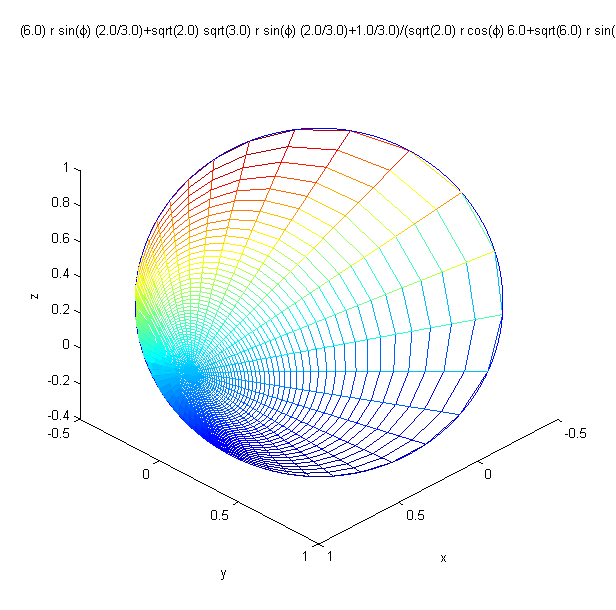
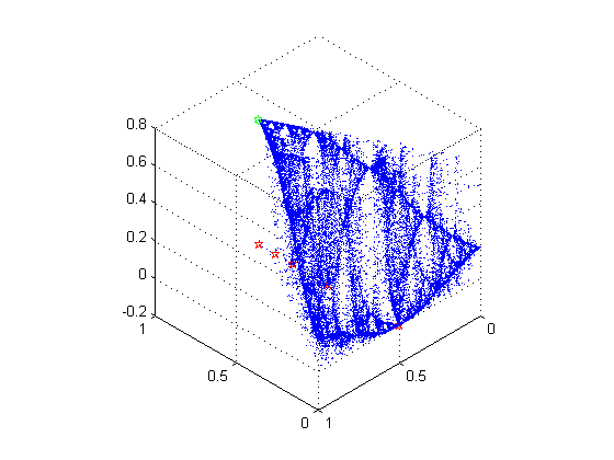
In Figure 7.2 we illustrate the geometric structure of by showing the image under of a uniform polar coordinate grid on the disk. and are similar, but are rotated through angles and .
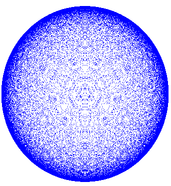
To obtain we apply all iterates of to the initial vector . In Figure 7.3 we show the result for . To better understand this distribution of points in the disk we examine its angular and radial projections.
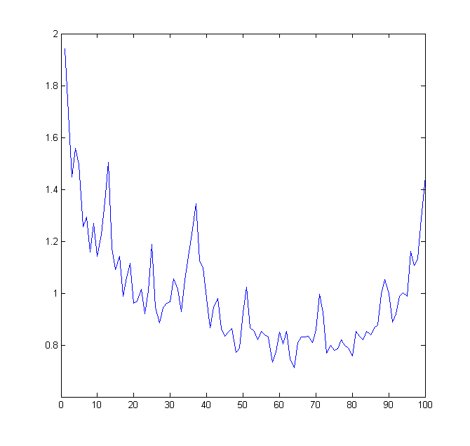
Introduce polar coordinates for the disk with (the origin corresponds to the vector ). The angular distribution at level is
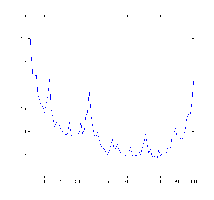
By symmetry it suffices to understand the distribution for . In Figure 7.4 we show histograms (100 slices) of on for and ; the values are normalized so that the average over all the values is .
Conjecture 7.1.
Let be defined as above. The limit of as is an absolutely continuous -invariant measure.
Similarly, the radial distribution at level is
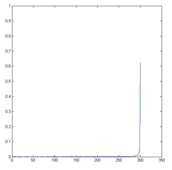
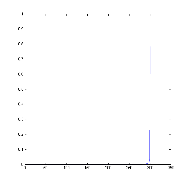
In Figure 7.5 we show histograms (300 bins) of on , for and ; the values are the ratios over the total number of vectors.
Conjecture 7.2.
Let be defined as above. The limit of as is the delta measure on the boundary .
We can say more about the mappings. Recall that we have defined
in Theorem 6.2. For each word , we have .
We first introduce the “polar coordinates” on the disk centered at on the plane . We know that is a parametrization of the unit circle lying on the plane. Put
which maps the unit circle lying on the plane to the unit circle lying on the plane . It follows that a parametrization of the circle of radius centered at on the plane is
| (7.1) |
With this parametrization, the image of radius under is
| (7.2) |
Thus if we take , we see that the image of the boundary circle is
| (7.3) |
Each maps the disk onto itself injectively. We first show that the mappings map the disk into itself. By (7.1) and (7.2), we need to see, by considering , whether to each pair , there exists a unique solution satisfying
The above reduces to
| (7.4) |
In particular,
| (7.5) |
so if , then and there is a solution satisfying (7.4). But by , we see that actually is also completely determined by ; it follows that the maps the disk onto itself injectively.
When we restrict the map on the boundary circle, we see from (7.5) that the circle is mapped onto itself and using the notations as before,
| (7.6) |
These show that corresponds to exactly one ; the map , referring to the restriction of to the boundary circle, given by is well-defined. Differentiating both equations in (7.6), we have . It follows that
and
Since and differ from a rotation, we have
We have the following theorem.
Theorem 7.3.
The mappings map the disk centered at of radius onto itself injectively. Further,
-
(i)
the mappings map the boundary circle centered at of radius onto itself; and
-
(ii)
If is the function in (7.1) which associates each to , there are differentiable maps satisfying given by
-
(iii)
Each has exactly two fixed points on the circle. The fixed points are, in “polar coordinates”, , for , , for and , for .
Proof.
We have already proved (i) and (ii). For (iii), we only need to prove for and the other two follow. By (ii), , are the only fixed points on the boundary circle. So it suffices to show that there is no fixed point in the open disk. Suppose, on the contrary, we have such a fixed point, say . Then we must have
which shows, since ,
but this contradicts the fact that . ∎
By (ii), We can regard and on the boundary circle as the same map under the parametrization (7.1).
If we directly view the maps as maps on the unit disk, we have an easy description on how they act on the unit disk.
Theorem 7.4.
Using the notation and as before. Let and be on the unit disk. Then maps every vertical line to a vertical line and every point with closer the boundary circle. In other words, if we denote to be the triangle with vertices , , , then every point in is mapped closer to the boundary by all of the three mappings and every point outside is mapped closer to the boundary by two of the mappings .
Proof.
The map on the unit disk is of the form
Fix a constant . If , then ; so maps every vertical line to a vertical line. Also, by (7.5), we have
thus if , and hence
The last assertion comes from the symmetry of , since all of these mappings differ by a rotation of and only. ∎
By Theorem 7.3, we can say more about the measure mentioned in Conjecture 7.1. We call the measure for some , for all . Recall that it is -invariant, hence
It follows that the function can be characterized by one satisfying the relation
If we consider separately, we have
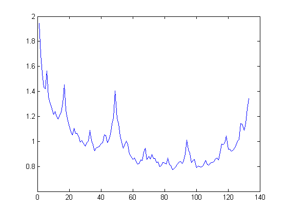
Finally, we give further experimental evidence for the conjectures. Conjecture 7.2 states that the radial distribution is the delta measure at ; the angular distribution on the whole disk should be the angular distribution on the boundary circle only. Pick three points , , from the three arcs mentioned in Theorem 7.4 respectively and iterate them times by all of the three maps. We cut the whole circle into 800 bins and plot the histogram for the number of points (normalized so that the average over all the values is ) in each bin for bins covering one sixth of the circle in Figure 7.6. This should be compared to Figure 7.4 which gives the level 13 histogram.
8. Acknowledgement
We are grateful to the referee for many useful suggestions.
References
- [1] Jonas Azzam, Michael A. Hall, Robert S. Strichartz, Conformal energy, conformal Laplacian, and energy measures on the Sierpinski gasket, Transactions of The American Mathematical Society , vol. 360, no. 04, pp. 2089-2131, 2007
- [2] O. Ben-Bassat, R.S.Strichartz and A. Teplyaev, What is not in the domain of the Laplacian on a Sierpinski gasket type fractal, J.Funct.Anal. 166, 197-217, 1999
- [3] Kyallee Dalrymple, Robert S. Strichartz and Jade P. Vinson, Fractal differential equations on the Sierpinski gasket, The Journal of Fourier Analysis and Applications, vol. 5, no. 2, pp. 203-284, 1999
- [4] Naotaka Kajino, Heat kernel asymptotics for the measurable Riemannian structure on the Sierpinski gasket, Potential Anal 36(2012), 67-115
- [5] Naotaka Kajino, Analysis and geometry of the measurable Riemannian structure on the Sierpinski gasket, preprint
- [6] J. Kigami, Measurable Riemannian geometry on the Sierpinski gasket: the Kusuoka measure and the Gaussian heat kernel estimate, Math, Ann. 340(2008), 781-804
- [7] R.D. Maudlin, S.C. Williams, Hausdorff dimension in graph directed constructions, Trans. Amer. Math. Soc 309(1988),811-829
- [8] Robert S. Strichartz, Differential equations on fractals: a tutorial, Princeton University Press, 2006
- [9] Robert S. Strichartz, Shu Tong Tse, Local behavior of smooth functions for the energy Laplacian on the Sierpinski gasket, Analysis 30(2010), 285-299
- [10] Alexander Teplyaev, Energy and Laplacian on the Sierpinski gasket, Proc. Symp. Pure Math 72 Part I (2004), 131-154
- [11] Alexander Teplyaev, Harmonic coordinates on fractals with finitely ramified cell structure, Canad. J. Math. 60(2008), 457-480