Engineering an Synthesis Tool
Abstract
The problem of reactive synthesis is to build a transducer, whose output is based on a history of inputs, such that, for every infinite sequence of inputs, the conjoint evolution of the inputs and outputs has a prefix that satisfies a given specification.
We describe the implementation of an synthesizer that outperforms existing tools on our benchmark suite. This is based on a new, direct translation from to a DFA represented as an array of Binary Decision Diagrams (MTBDDs) sharing their nodes. This MTBDD-based representation can be interpreted directly as a reachability game that is solved on-the-fly during its construction.
1 Introduction
Reactive synthesis is concerned with synthesizing programs (a.k.a. strategies) for reactive computations (e.g., processes, protocols, controllers, robots) in active environments [47, 30, 26], typically, from temporal logic specifications. In AI, Reactive Synthesis, which is related to (strong) planning for temporally extended goals in fully observable nondeterministic domains [16, 3, 4, 14, 6, 34, 21, 15], has been studied with a focus on logics on finite traces such as [33, 7, 22, 23]. In fact, synthesis [23] is one of the two main success stories of reactive synthesis so far (the other being the GR(1) fragment of LTL [46]), and has brought about impressive advances in scalability [56, 8, 18, 20].
Reactive synthesis for involves the following steps [23]: (1) distinguishing uncontrollable input () and controllable output () variables in an specification of the desired system behavior; (2) constructing a DFA accepting the behaviors satisfying ; (3) interpreting this DFA as a two-player reachability game, and finding a controller winning strategy. Step (2) has two main bottlenecks: the DFA is worst-case doubly-exponential and its propositional alphabet is exponential. The first only happens in the worst case, while the second blow-up – which we call alphabet explosion – always happens.
Mona [39] addresses the alphabet-explosion problem, which happens also in MSO, by representing a DFA with Multi-Terminal Binary Decision Diagrams (MTBDDs) [36]. MTBDDs are a variant of BDDs [12] with arbitrary terminal values. If terminal values encode destination states, an MTBDD can compactly represent all outgoing transitions of a single DFA state. A DFA is represented, through its transition function, as an array of MTBDDs sharing their nodes.
The first synthesizer, Syft [56], converted into first-order logic in order to build a MTBDD-encoded DFA with Mona. Syft then converted this DFA into a BDD representation to solve the reachability game using a symbolic fixpoint computation. Syft demonstrated that DFA construction is the main bottleneck in synthesis, motivating several follow-up efforts.
One approach to effective DFA construction uses compositional techniques, decomposing the input formula into smaller subformulas whose DFAs can be minimized before being recombined. Lisa [8] decomposes top-level conjunctions, while Lydia [19] and LydiaSyft [29] decompose every operator.
Compositional methods construct the full DFA before synthesis can proceed, limiting their scalability. On-the-fly approaches [53] construct the DFA incrementally, while simultaneously solving the game, allowing strategies to be found before the complete DFA is built. The DFA construction may use various techniques. Cynthia [20] uses Sentential Decision Diagrams (SDDs) [17] to generate all outgoing transitions of a state at once. Alternatively, Nike [28] and MoGuSer [54] use a SAT-based method to construct one successor at a time. The game is solved by forward exploration with suitable backpropagation.
Contributions and Outline In Section 3, we propose a direct and efficient translation from to MTBDD-encoded DFA (henceforth called MTDFA). In Section 4, we show that given an appropriate ordering of BDD variables, realizability can be solved by interpreting the MTBDD nodes of the MTDFA as the vertices of a reachability game, known to be solvable in linear time by backpropagation of the vertices that are winning for the output player. We give a linear-time implementation for solving the game on-the-fly while it is constructed. For more opportunities to abort the on-the-fly construction earlier, we additionally backpropagate vertices that are known to be winning by the input player. We implemented these techniques in two tools (ltlf2dfa \faExternalLink* and ltlfsynt \faExternalLink*) that compare favorably with other existing tools in benchmarks from the -Synthesis Competition. To meet space limits, Section 5 only reports on the realizability benchmark, and we refer readers to our artifact for the other results [24].
2 Preliminaries
2.1 Words over Assignments
A word over of length over an alphabet is a function . We use (resp. and ) to denote the set of words of length (resp. any length and ). We use to represent the length of a word . For and , denotes the prefix of of length .
Let be a finite set of Boolean variables (a.k.a. atomic propositions). We use to denote the set of all assignments, i.e., functions mapping variables to values in .
Given two disjoint sets of variables and , and two assignments and , we use to denote their combination.
In a system modeled using discrete Boolean signals that evolve synchronously, we assign a variable to each signal, and use a word over assignments of to represent the conjoint evolution of all signals over time.
We extend to such words. For two words , of length over assignments that use disjoint sets of variables, we use to denote a word such that for .
2.2 Linear Temporal Logic over Finite, Nonempty Words.
We use classical semantics over nonempty finite words [22].
Definition 1 ( formulas)
An formula is built from a set of variables, using the following grammar where , and is any Boolean operator: .
Symbols and represent the true and false formulas. Temporal operators are (weak next), (strong next), (until), (release), (globally), and (finally). denotes the set of formulas produced by the above grammar. We use to denote the set of subformulas for . A maximal temporal subformula of is a subformula whose primary operator is temporal and that is not strictly contained within any other temporal subformula of .
The satisfaction of a formula by word of length at position , denoted , is defined as follows.
The set of words that satisfy is .
Example 1
Consider the following formulas over : , and . If we interpret as input signals, and as output signals, formula specifies a 1-bit multiplexer: the value of the signal should be equal to the value of either or depending on the setting of . Formula specifies that the last value of should be if and only if was at some instant.
Definition 2 (Propositional Equivalence [27])
For , let be the Boolean formula obtained from by replacing every maximal temporal subformula by a Boolean variable . Two formulas are propositionally equivalent, denoted , if and are equivalent Boolean formulas.
Example 2
Formulas and are propositionally equivalent. Indeed, .
Note that implies , but the converse is not true in general. Since is an equivalence relation, we use to denote some unique representative of the equivalence class of with respect to .
2.3 Realizability
Our goal is to build a tool that decides whether an formula is realizable.
Definition 3 ([23, 37])
Given two disjoint sets of variables (inputs) and (outputs), a controller is a function , that produces an assignment of output variables given a history of assignments of input variables.
Given a word of input assignments , the controller can be used to generate a word of output assignments . The definition of may use two semantics depending on whether we want to the controller to have access to the current input assignment to decide the output assignment:
- Mealy semantics:
-
for all .
- Moore semantics:
-
for all .
A formula is said to be Mealy-realizable or Moore-realizable if there exists a controller such that for any word there exists a position such that using the desired semantics.
Example 3
Formula (from Example 1) is Mealy-realizable but not Moore-realizable. Formula is both Mealy and Moore-realizable.
2.4 Multi-Terminal BDDs
Let be a finite set. Given a finite set of variables (that are implicitly ordered by their index) we use to denote a function that maps an assignment of all those variables to an element of . Given a variable and a Boolean , the function represents a generalized co-factor obtained by replacing by in . When , a function can be encoded into a Binary Decision Diagram (BDD) [11]. Multi-Terminal Binary Decision Diagrams (MTBDDs) [44, 45, 32, 39], also called Algebraic Decision Diagrams (ADDs) [5, 51], generalize BDDs by allowing arbitrary values on the leaves of the graph.
A Multi-Terminal BDD encodes any function as a rooted, directed acyclic graph. We use the term nodes to refer to the vertices of this graph. All nodes in an MTBDD are represented by triples of the form . In an internal node, and point to successors MTBDD nodes called the and links. The intent is that if is the root of the MTBDD representing the function , then and are the roots of the MTBDDs representing the functions and , respectively. Leaves of the graph, called terminals, hold values in . For consistency with internal nodes, we represent terminals with a triple of the form where . When comparing the first elements of different triplets, we assume that is greater than all variables. We use to denote the set of MTBDD nodes that can appear in the representation of an arbitrary function .
Following the classical implementations of BDD packages [11, 1], we assume that MTBDDs are ordered (variables of are ordered and visited in increasing order by all branches of the MTBDD) and reduced (isomorphic subgraphs are merged by representing each triplet only once, and internal nodes with identical and links are skipped over). Doing so ensures that each function has a unique MTBDD representation for a given order of variables.
Given and an assignment , we note the element of stored on the terminal of that ††margin: Cf. App. 0.A.1 is reached after following the assignment in the structure of . We use to denote the number of MTBDD nodes that can be reached from .
Let and be two MTBDD nodes representing functions , and let , be a binary operation. One can easily construct representing the function , by generalizing the apply2 function typically found in BDD libraries [32].††margin: Cf. App. 0.A.2 We use to denote the MTBDD that results from this construction.
For we use to denote the elements of that label terminals reachable from . This set can be computed in .††margin: Cf. App. 0.A.3.
2.5 MTBDD-Based Deterministic Finite Automata
We now define an MTBDD-based representation of a DFA with a propositional alphabet, inspired by Mona’s DFA representation [36, 39].
Definition 4 (MTDFA)
An MTDFA is a tuple , where is a finite set of states, is a finite (and ordered) set of variables, is the initial state, represents the set of outgoing transitions of each state. For a word of length , let be a sequence of pairs defined recursively as follows: , and for , is the pair reached by evaluating assignment on . The word is accepted by iff . The language of , denoted , is the set of words accepted by .
Example 4
Figure 1 shows an MTDFA where . The set of states are the dashed rectangles on the left. For each such a state , the dashed arrow points to the MTBDD node representing . The MTBDD nodes are shared between all states. If, starting from the initial state at the top-left, we read the assignment , we should follow only the links (plain arrows) and we reach the accepting terminal. If we read this assignment a second-time, starting this time from state on the left, we reach the same accepting terminal. Therefore, non-empty words of the form are accepted by this automaton.
An MTDFA can be regarded as a semi-symbolic representation of a DFA over propositional alphabet.††margin: Cf. App. 0.C From a state and reading the assignment , the automaton jumps to the state that is the result of computing . The value of indicates whether that assignment is allowed to be the last one of the word being read. By definition, an MTDFA cannot accept the empty word.
MTDFAs are compact representations of DFAs, because the MTBDD representation of the successors of each state can share their common nodes. Boolean operations can be implemented over MTDFAs, with the expected semantics, i.e., .††margin: Cf. App. 0.B
3 Translating to MTBDD and MTDFA
This section shows how to directly transform a formula into an MTDFA such that . The translation is reminiscent of other translations of to DFA [22, 20], but it leverages the fact that MTBBDs can provide a normal form for formulas.
The construction maps states to formulas, i.e., . Terminals appearing in the MTBDDs of will be labeled by pairs , so we use to shorten the notation from Section 2.4.
The conversion from to is based on the
function defined
inductively as follows:
Boolean operators that appear to the right of the equal sign are applied on MTBDDs as discussed in Section 2.4. Terminals in are combined with: and .
Theorem 3.1
For , let be the MTDFA obtained by setting , , and letting be the smallest subset of such that , and such that for any and for any , then . With this construction, is finite and .
Proof
(sketch) By definition of , contains only Boolean combinations of subformulas of . Propositional equivalence implies that the number of such combinations is finite: . The language equivalence follows from the definition of , and from some classical equivalences. For instance the rule for is based on the equivalence .
Example 5
The definition of as an MTBDD representation of the set of successors of a state can be thought as a symbolic representation of Antimirov’s linear forms [2] for DFA with propositional alphabets. Antimirov presented linear forms as an efficient way to construct all (partial) derivatives at once, without having to iterate over the alphabet. For , formula progressions [20] are the equivalent of Brozozowski derivatives [13]. Here, computes all formulas progressions at once, without having to iterate over an exponential number of assignments.
Finally, note that while this construction works with any order for , different orders might produce a different number of MTBDD nodes.
Optimizations
The previous definitions can be improved in several ways.
Our implementation of MTBDD actually supports terminals that are the Boolean terminals of standard BDDs as well as the terminals used so far. So we are actually using , and we encode and directly as and respectively. With those changes, apply2 may be modified to shortcut the recursion depending on the values of , , and . For instance if and , then can be returned immediately. ††margin: Cf. App 0.A.4 Such shortcuts may be implemented for regardless of the nature of , so our implementation of MTBDD operations is independent of .
When combining terminals during the computation of , one has to
compute the representative formula .
This can be done by converting and into
BDDs, keeping track of such conversions in a hash table. Two
propositionally equivalent formulas will have the same BDD
representation. While we are looking for a representative formula, we
can also use the opportunity to simplify the formula at hand. We
use the following very simple rewritings, for patterns that occur
naturally in the output of :
, , , .
Once has been built, two states such that can be merged by replacing all occurrences of by in the leaves of .
4 Deciding Realizability
realizability (Def. 3) is solved by reducing the problem to a two-player reachability game where one player decides the input assignments and the other player decides the output assignments [23]. Section 4.1 presents reachability games and how to interpret the MTDFA as a reachability game, and Section 4.2 shows how we can solve the game on-the-fly while constructing it.
4.1 Reachability Games & Backpropagation
Definition 5 (Rechability Game)
A Reachability Game is , where is a finite set of vertices partitioned to player output (abbreviated o) and player input (abbreviated i), is a finite set of edges, and is the set of target states. Let . This graph is also referred to as the game arena.
A strategy for player o is a cycle-free subgraph such that (a) for every we have or and (b) if then . A vertex is winning for o if for some strategy .
Such a reachability game can be solved by backpropagation identifying the maximal set in a strategy. Namely, start from . Then is iteratively augmented with every vertex in that has some edge to , and every (non dead-end) vertex in whose edges all lead to . At the end of this backpropagation, which can be performed in linear time [35, Theorem 3.1.2], every vertex in is winning for o, and every vertex outside is losing for o. Notice that every dead-end that is not in cannot be winning. It follows that we can identify some (but not necessarily all) vertices that are losing by setting as the set of all dead-ends and adding to every vertex that has some edge to and every vertex whose edges all lead to .
Let be a translation of (per Th. 3.1) such that variables of appear before in the MTBDD encoding of .
Definition 6 (Realizability Game)
We define the reachability game in which corresponds the set of nodes that appear in the MTBDD encoding of . contains all nodes such that or (terminals), and contains those with . The edges follows the structure of , i.e., if has a node , then . Additionally, for any terminal such that , contains the edge . Finally, is the set of accepting terminals, i.e., nodes of the form .
Theorem 4.1
Vertex is winning for o in iff is Mealy-realizable.
Moore realizability can be checked similarly by changing the order of and in the MTBDD encoding of .
Example 7
Figure 2 shows how to interpret the MTDFA of Figure 1 as a game, by turning each MTBDD node into a game vertex. The player owning each vertex is chosen according to the variable that labels it. Vertices corresponding to accepting terminals become winning targets for the output player, so the game stops once they are reached. Solving this game will find every internal node as winning for o, so the corresponding formula is Mealy-realizable.
The difference with DFA games [23, 20, 28, 54] is that instead of having player i select all input signals at once, and then player o select all output signals at once, our game proceeds by selecting one signal at a time. Sharing nodes that represent identical partial assignments contributes to the scalability of our approach.
4.2 Solving Realizability On-the-fly
We now show how to construct and solve on-the-fly, for better efficiency. The construction is easier to study in two parts: (1) the on-the-fly solving of reachability games, based on backpropagation, and (2) the incremental construction of , done with a forward exploration of a subset of the MTDFA for .
Algorithm 1 presents the first part: a set of functions for constructing a game arena incrementally, while performing the ††margin: Cf. App. 0.D linear-time backpropagation algorithm on-the-fly. At all points during this construction, the winning status of a vertex () will be one of o (player o can force the play to reach , i.e., the vertex belongs to ), i (player i can force the play to avoid , i.e., the vertex belongs to ), or u (undetermined yet), and the algorithm will backpropagate both o and i. At the end of the construction, all vertices with status u will be considered as winning for i. Like in the standard algorithm for solving reachability games [35, Th. 3.1.2] each state uses a counter (, lines 1,1) to track the number of its undeterminated successors. When a vertex is marked as winning for player by calling set_winner(x,w), an undeterminated predecessor has its counter decreased (line 1), and can be marked as winning for (line 1) if either vertex is owned by (player can choose to go to ) or the counter dropped to (meaning that all choices at were winning for ).
To solve the game while it is constructed, we freeze vertices. A vertex should be frozen after all its successors have been introduced with new_edge. The counter dropping to is only checked on frozen vertices (lines 1, 1) since it is only meaningful if all successors of a vertex are known.
Algorithm 2 is the second part. It shows how to build incrementally. It translates the states of the corresponding MTDFA one at a time, and uses the functions of Algorithm 1 to turn each node of into a vertex of the game. Since the functions of Algorithm 1 update the winning status of the states as soon as possible, Algorithm 2 can use that to cut parts of the exploration.
Instead of using as initial vertex of the game, as in Theorem 4.1, we consider as initial vertex (line 2): this makes no theoretical difference, since has as unique successor. Lines 2,2–2,2, and 2 implements the exploration of all the formulas that would label the states of the MTDFA for (as needed to implement Theorem 3.1). The actual order in which formulas are removed from on line 2 is free. (We found out that handling as a queue to implement a BFS exploration worked marginally better than using it as a stack to do a DFS-like exploration, so we use a BFS in practice.)
Each is translated into an MTBDD representing its possible successors. The constructed game should have one vertex per MTBDD node in . Those vertices are created in the inner while loop (lines 2–2). Function declare_vertex is used to assign the correct owner to each new node according to its decision variable (as in Def. 6) as well as adding those nodes to the set processed by this inner loop. Terminal nodes are either marked as winning for one of the players (lines 2–2) or stored in (line 2).
Since connecting game vertices may backpropagate their winning status, the encoding loop can terminate early whenever the vertex associated to becomes determined (lines 2 and 2). If that vertex is not determined, the of are added to (line 2) for further exploration.
The entire construction can also stop as soon as the initial vertex is determined (line 2). However, if the algorithm terminates with , it still means that o cannot reach its targets. Therefore, as tested by line 2, formula is realizable iff in the end.
Theorem 4.2
Algorithm 2 returns iff is Mealy-realizable.
5 Implementation and Evaluation
Our algorithms have been implemented in Spot [25], after extending its fork of BuDDy [42] to support MTBDDs. ††margin: Cf. App. 0.F The release of Spot 2.14 distributes two new command-line tools: ltlf2dfa \faExternalLink* and ltlfsynt \faExternalLink*, implementing translation from to MTDFA, and solving synthesis. We describe and evaluate ltlfsynt in the following.
Preprocessing
Before executing Algorithm 2, we use a few preprocessing techniques to simplify the problem. We remove variables that always have the same polarity in the specification (a simplification used also by Strix [50]), and we decompose the specifications into output-disjoint sub-specifications that can be solved independently [31]. A specification such as , from Example 1, is not solved directly as demonstrated here, but split into two output-disjoint specifications and that are solved separately. Finally, we also simplify formulas using very simple rewriting ††margin: Cf. App. 0.G rules such as that reduce the number of MTBDD operations required during translation.
One-step (un)realizability checks
An additional optimization consists in performing one-step realizability and one-step unrealizability checks in Algorithm 2. ††margin: Cf. App. 0.H The principle is to transform the formula into two smaller Boolean formulas and , such that if is realizable it implies that is realizable, and if is unrealizable it implies that is unrealizable [53, Theorems 2–3]. Those Boolean formulas can be translated to BDDs for which realizability can be checked by quantification. On success, it avoids the translation of the larger formula . The simple formula of our running example is actually one-step realizable.
Synthesis
After deciding realizability, ltlfsynt is able to extract a strategy from the solved game in the form of a Mealy machine, and encode that into an And-Invert Graph (AIG) [10]: the expected output of the Synthesis Competition for the synthesis tracks. The conversion from Mealy to AIG reuses prior work [48, 49] developed for Spot’s LTL (not ) synthesis tool. We do not detail nor evaluate these extra steps here due to lack of space.
Evaluation
We evaluated the task of deciding reachability over specifications from the Synthesis Competition [38]. We took all tlsf-fin specifications from SyntComp’s repository \faExternalLink*, excluded some duplicate specifications as well as some specifications that were too large to be solved by any tool, and converted the specifications from TLSF v1.2 [37] to using syfco [37].
We used BenchExec 3.22 [9] to track time and memory usage of each tool. Tasks were run on a Core i7-3770 with Turbo Boost disabled, and frequency scaled down to 1.6GHz to prevent CPU throttling. The computer has 4 physical cores and 16GB of memory. BenchExec was configured to run up to 3 tasks in parallel with a memory limit of 4GB per task, and a time limit of 15 minutes.
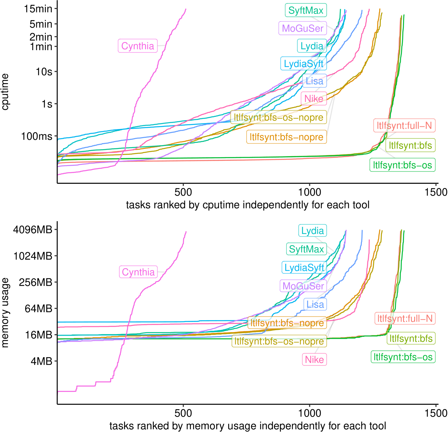
Figure 3 compares five configurations of ltlfsynt against seven other tools. ††margin: More in App. 0.I. We verified that all tools were in agreement. Lydia 0.1.3 [19], SyftMax (or Syft 2.0) [55] and LydiaSyft 0.1.0-alpha [29] are all using Mona to construct a DFA by composition; they then solve the resulting game symbolically after encoding it using BDDs. Lisa [8] uses a hybrid compositional construction, mixing explicit compositions (using Spot), with symbolic compositions (using BuDDy), solving the game symbolically in the end. Cynthia 0.1.0 [20], Nike 0.1.0 [28], and MoGuSer [54] all use an on-the-fly construction of a DFA game that they solve via forward exploration with backpropagation, but they do not implement backpropagation in linear time, as we do. Yet, the costly part of synthesis is game generation, not solving. Cynthia uses SDDs [17] to compute successors and represent states, while Nike and MoGuSer use SAT-based techniques to compute successors and BDDs to represent states. Nike, Lisa, and LydiaSyft were the top-3 contenders of the track of SyntComp in 2023 and 2024.
Configuration ltlfsynt:bfs-nopre corresponds to Algorithm 2 were is a queue: it already solves more cases than all other tested tools. Suffix -nopre indicates that preprocessings of the specification are disabled (this makes comparison fairer, since other tools have no such preprocessings). The version with preprocessings enabled is simply called ltlfsynt:bfs. Variants with “-os” adds the one-step (un)realizability checks that LydiaSyft, Cynthia, and Nike also perform.
We also include a configuration ltlfsynt:full-N that corresponds to first translating the specification into a MTDFA using Theorem 3.1, and then solving the game by linear propagation. The difference between ltlfsynt:full and ltlfsynt:bfs shows the gain obtained with the on-the-fly translation: although that look small in the cactus plot, it is important in some specifications.††margin: Tab. 2–3 in App. 0.I.
Data Availability Statement
Implementation, supporting scripts, detailed analysis of this benchmark, and additional examples are archived on Zenodo [24].
6 Conclusion
We have presented the implementation of ltlfsynt, and evaluated it to be faster at deciding realizability than seven existing tools, including the winners of SyntComp’24. The implementation uses a direct and efficient translation from to DFA represented by MTBDDs, which can then be solved as a game played directly on the structure of the MTBDDs. The two constructions (translation and game solving) are performed together on-the-fly, to allow early termination.
Although ltlsynt also includes a preliminary implementation of synthesis of And-Inverter graphs, we leave it as future work to document it and ensure its correctness.
Finally, the need for solving a reachability game while it is discovered also occurs in other equivalent contexts such as HornSAT, where linear algorithms that do not use “counters” and “predecessors” (unlike ours) have been developed [43]. Using such algorithms might improve our solution by saving memory.
References
- [1] Andersen, H.R.: An introduction to binary decision diagrams. Lecture notes for Efficient Algorithms and Programs, Fall 1999 (1999), https://web.archive.org/web/20090530154634/http://www.itu.dk:80/people/hra/bdd-eap.pdf
- [2] Antimirov, V.: Partial derivatives of regular expressions and finite automaton constructions. Theoretical Computer Science 155(2), 291–319 (Mar 1996). https://doi.org/10.1016/0304-3975(95)00182-4
- [3] Bacchus, F., Kabanza, F.: Planning for temporally extended goals. Annals of Mathematics and Artificial Intelligence 22, 5–27 (1998). https://doi.org/10.1023/A:1018985923441
- [4] Bacchus, F., Kabanza, F.: Using temporal logics to express search control knowledge for planning. Artificial Intelligence 116(1–2), 123–191 (2000). https://doi.org/10.1016/S0004-3702(99)00071-5
- [5] Bahar, R.I., Frohm, E.A., Gaona, C.M., Hachtel, G.D., Macii, E., Pardo, A., Somenzi, F.: Algebraic decision diagrams and their applications. In: Proceedings of 1993 International Conference on Computer Aided Design (ICCAD’93). pp. 188–191. IEEE Computer Society Press (Nov 1993). https://doi.org/10.1109/ICCAD.1993.580054
- [6] Baier, J.A., Fritz, C., McIlraith, S.A.: Exploiting procedural domain control knowledge in state-of-the-art planners. In: Proceedings of the International Conference on Automated Planning and Scheduling (ICAPS’07). pp. 26–33. AAAI (2007), https://aaai.org/papers/icaps-07-004
- [7] Baier, J.A., McIlraith, S.A.: Planning with first-order temporally extended goals using heuristic search. In: Proceedings of the 21st national conference on Artificial intelligence (AAAI’06). pp. 788–795. AAAI Press (2006). https://doi.org/10.5555/1597538.1597664
- [8] Bansal, S., Li, Y., Tabajara, L.M., Vardi, M.Y.: Hybrid compositional reasoning for reactive synthesis from finite-horizon specifications. In: Proceedings of the 34th national conference on Artificial intelligence (AAAI’20). pp. 9766–9774. AAAI Press (2020). https://doi.org/10.1609/AAAI.V34I06.6528
- [9] Beyer, D., Löwe, S., Wendler, P.: Reliable benchmarking: requirements and solutions. International Journal on Software Tools for Technology Transfer 21, 1–29 (Feb 2019). https://doi.org/10.1007/s10009-017-0469-y
- [10] Biere, A., Heljanko, K., Wieringa, S.: AIGER 1.9 and beyond. Tech. Rep. 11/2, Institute for Formal Models and Verification, Johannes Kepler University, Altenbergerstr. 69, 4040 Linz, Austria (2011), https://fmv.jku.at/aiger/
- [11] Bryant, R.E.: Graph-based algorithms for boolean function manipulation. IEEE Transactions on Computers 35(8), 677–691 (Aug 1986). https://doi.org/10.1109/TC.1986.1676819
- [12] Bryant, R.E.: Symbolic boolean manipulation with ordered binary-decision diagrams. ACM Comput. Surv. 24(3), 293–318 (Sep 1992). https://doi.org/10.1145/136035.136043
- [13] Brzozowski, J.A.: Derivatives of regular expressions. Journal of the ACM 11(4), 481–494 (Oct 1964). https://doi.org/10.1145/321239.321249
- [14] Calvanese, D., De Giacomo, G., Vardi, M.Y.: Reasoning about actions and planning in LTL action theories. In: Proceedings of the Eights International Conference on Principles of Knowledge Representation and Reasoning (KR’02). pp. 593–602. Morgan Kaufmann (2002). https://doi.org/10.5555/3087093.3087142
- [15] Camacho, A., Bienvenu, M., McIlraith, S.A.: Towards a unified view of AI planning and reactive synthesis. In: Proceedings of the 29th International Conference on Automated Planning and Scheduling (ICAPS’19). pp. 58–67. AAAI Press (2019). https://doi.org/10.1609/icaps.v29i1.3460
- [16] Cimatti, A., Pistore, M., Roveri, M., Traverso, P.: Weak, strong, and strong cyclic planning via symbolic model checking. Artificial Intelligence 147(1–2), 35–84 (2003). https://doi.org/10.1016/S0004-3702(02)00374-0
- [17] Darwiche, A.: SDD: A new canonical representation of propositional knowledge bases. In: Proceedings of the 22nd International Joint Conference on Artificial Intelligence. pp. 819–826. AAAI Press (2011). https://doi.org/10.5591/978-1-57735-516-8/IJCAI11-143
- [18] De Giacomo, G., Favorito, M.: Compositional approach to translate LTLf/LDLf into deterministic finite automata. In: Proceedings of the 31st International Conference on Automated Planning and Scheduling (ICAPS’21). pp. 122–130 (2021). https://doi.org/10.1609/icaps.v31i1.15954
- [19] De Giacomo, G., Favorito, M.: Compositional approach to translate LTLf/LDLf into deterministic finite automata. In: Biundo, S., Do, M., Goldman, R., Katz, M., Yang, Q., Zhuo, H.H. (eds.) Proceedings of the 31’st International Conference on Automated Planning and Scheduling (ICAPS’21). pp. 122–130. AAAI Press (Aug 2021). https://doi.org/10.1609/icaps.v31i1.15954
- [20] De Giacomo, G., Favorito, M., Li, J., Vardi, M.Y., Xiao, S., Zhu, S.: LTLf synthesis as AND-OR graph search: Knowledge compilation at work. In: Raedt, L.D. (ed.) Proceedings of the 31st International Joint Conference on Artificial Intelligence (IJCAI’22). pp. 2591–2598. International Joint Conferences on Artificial Intelligence Organization (Jul 2022). https://doi.org/10.24963/ijcai.2022/359
- [21] De Giacomo, G., Rubin, S.: Automata-theoretic foundations of fond planning for LTLf/LDLf goals. In: Proceedings of the 27th International Joint Conference on Artificial Intelligence (IJCAI’18). pp. 4729–4735 (2018). https://doi.org/10.24963/ijcai.2018/657
- [22] De Giacomo, G., Vardi, M.Y.: Linear temporal logic and linear dynamic logic on finite traces. In: Proceedings of the 23rd International Joint Conference on Artificial Intelligence (IJCAI’13). pp. 854–860. IJCAI’13, AAAI Press (Aug 2013). https://doi.org/10.5555/2540128.2540252
- [23] De Giacomo, G., Vardi, M.Y.: Synthesis for LTL and LDL on finite traces. In: Proceedings of the 24th International Joint Conference on Artificial Intelligence (IJCAI’15). pp. 1558–1564. AAAI Press (2015). https://doi.org/10.5555/2832415.2832466
- [24] Duret-Lutz, A.: Supporting material for ”Engineering an LTLf Synthetizer Tool” (2025). https://doi.org/10.5281/zenodo.15752968
- [25] Duret-Lutz, A., Renault, E., Colange, M., Renkin, F., Aisse, A.G., Schlehuber-Caissier, P., Medioni, T., Martin, A., Dubois, J., Gillard, C., Lauko, H.: From Spot 2.0 to Spot 2.10: What’s new? In: Proceedings of the 34th International Conference on Computer Aided Verification (CAV’22). Lecture Notes in Computer Science, vol. 13372, pp. 174–187. Springer (Aug 2022). https://doi.org/10.1007/978-3-031-13188-2_9
- [26] Ehlers, R., Lafortune, S., Tripakis, S., Vardi, M.Y.: Supervisory control and reactive synthesis: a comparative introduction. Discrete Event Dynamic Systems 27(2), 209–260 (2017). https://doi.org/10.1007/s10626-015-0223-0
- [27] Esparza, J., Křetínský, J., Sickert, S.: One theorem to rule them all: A unified translation of LTL into -automata. In: Dawar, A., Grädel, E. (eds.) Proceedings of the 33rd Annual ACM/IEEE Symposium on Logic in Computer Science (LICS’18). pp. 384–393. ACM (2018). https://doi.org/10.1145/3209108.3209161
- [28] Favorito, M.: Forward LTLf synthesis: DPLL at work. In: Benedictis, R.D., Castiglioni, M., Ferraioli, D., Malvone, V., Maratea, M., Scala, E., Serafini, L., Serina, I., Tosello, E., Umbrico, A., Vallati, M. (eds.) Proceedings of the 30th Workshop on Experimental evaluation of algorithms for solving problems with combinatorial explosion (RCRA’23). CEUR Workshop Proceedings, vol. 3585 (2023), https://ceur-ws.org/Vol-3585/paper7_RCRA4.pdf
- [29] Favorito, M., Zhu, S.: LydiaSyft: A compositional symbolic synthesis framework for LTLf specifications. In: Proceedings of the 31st International Conference on Tools and Algorithms for the Construction and Analysis of Systems (TACAS’25). Lecture Notes in Computer Science, vol. 15696, pp. 295–302. Springer (May 2025). https://doi.org/10.1007/978-3-031-90643-5_15
- [30] Finkbeiner, B.: Synthesis of reactive systems. In: Javier Esparza, Orna Grumberg, S.S. (ed.) Dependable Software Systems Engineering, NATO Science for Peace and Security Series — D: Information and Communication Security, vol. 45, pp. 72–98. IOS Press (2016). https://doi.org/10.3233/978-1-61499-627-9-72
- [31] Finkbeiner, B., Geier, G., Passing, N.: Specification decomposition for reactive synthesis. In: Proceedings for the 13th NASA Formal Methods Symposium (NFM’21). Lecture Notes in Computer Science, vol. 12673, pp. 113–130. Springer (2021). https://doi.org/10.1007/978-3-030-76384-8_8
- [32] Fujita, M., McGeer, P.C., Yang, J.C.: Multi-terminal binary decision diagrams: An efficient data structure for matrix representation. Formal Methods in System Design 10(2/3), 149–169 (1997). https://doi.org/10.1023/A:1008647823331
- [33] Gabbay, D., Pnueli, A., Shelah, S., Stavi, J.: On the temporal analysis of fairness. In: Proceedings of the 7th ACM SIGPLAN-SIGACT symposium on Principles of programming languages (POPL’80). pp. 163–173. Association for Computing Machinery (1980). https://doi.org/doi.org/10.1145/567446.5674
- [34] Gerevini, A., Haslum, P., Long, D., Saetti, A., Dimopoulos, Y.: Deterministic planning in the fifth international planning competition: PDDL3 and experimental evaluation of the planners. Artificial Intelligence 173(5–6), 619–668 (2009). https://doi.org/10.1016/j.artint.2008.10.012
- [35] Grädel, E.: Finite model theory and descriptive complexity. In: Finite Model Theory and Its Applications, chap. 3, pp. 125–230. Texts in Theoretical Computer Science an EATCS Series, Springer Berlin Heidelberg, Berlin, Heidelberg (2007). https://doi.org/10.1007/3-540-68804-8_3
- [36] Henriksen, J.G., Jensen, J., Jørgensen, M., Klarlund, N., Paige, R., Rauhe, T., Sandholm, A.: Mona: Monadic second-order logic in practice. In: Brinksma, E., Cleaveland, W.R., Larsen, K.G., Margaria, T., Steffen, B. (eds.) First International Workshop on Tools and Algorithms for the Construction and Analysis of Systems (TACAS’95). pp. 89–110. Springer Berlin Heidelberg (1995). https://doi.org/10.1007/3-540-60630-0_5
- [37] Jacobs, S., Perez, G.A., Schlehuber-Caissier, P.: The temporal logic synthesis format TLSF v1.2. arXiV (2023). https://doi.org/10.48550/arXiv.2303.03839
- [38] Jacobs, S., Perez, G.A., Abraham, R., Bruyère, V., Cadilhac, M., Colange, M., Delfosse, C., van Dijk, T., Duret-Lutz, A., Faymonville, P., Finkbeiner, B., Khalimov, A., Klein, F., Luttenberger, M., Meyer, K.J., Michaud, T., Pommellet, A., Renkin, F., Schlehuber-Caissier, P., Sakr, M., Sickert, S., Staquet, G., Tamines, C., Tentrup, L., Walker, A.: The reactive synthesis competition (SYNTCOMP): 2018–2021. arXiV (Jun 2022). https://doi.org/10.48550/ARXIV.2206.00251
- [39] Klarlund, N., Møller, A.: MONA version 1.4, user manual. Tech. rep., BRICS (Jul 2001), https://www.brics.dk/mona/mona14.pdf
- [40] Klarlund, N., Rauhe, T.: BDD algorithms and cache misses. Tech. Rep. BR-96-26, BRICS (Jul 1996), https://www.brics.dk/mona/papers/bdd-alg-cache-miss/article.pdf
- [41] Kluyver, T., Ragan-Kelley, B., Pérez, F., Granger, B., Bussonnier, M., Frederic, J., Kelley, K., Hamrick, J., Grout, J., Corlay, S., Ivanov, P., Avila, D., Abdalla, S., Willing, C., development team, J.: Jupyter notebooks — a publishing format for reproducible computational workflows. In: Loizides, F., Scmidt, B. (eds.) Proceedings of 20th International Conference on Electronic Publishing: Positioning and Power in Academic Publishing: Players, Agents and Agendas (ELPUB’16). pp. 87–90. IOS Press (2016). https://doi.org/10.3233/978-1-61499-649-1-87
- [42] Lind-Nielsen, J.: BuDDy: A binary decision diagram package. User’s manual. (1999), https://web.archive.org/web/20040402015529/http://www.itu.dk/research/buddy/
- [43] Liu, X., Smolka, S.A.: Simple linear-time algorithms for minimal fixed points. In: Larsen, K.G., Skyum, S., Winskel, G. (eds.) Proceedings of the 25th International Colloquium on Automata, Languages and Programming (ICALP’98). pp. 53–66. Springer Berlin Heidelberg (1998). https://doi.org/10.1007/BFb0055035
- [44] Long, D.: BDD library. source archive, https://www.cs.cmu.edu/˜modelcheck/bdd.html
- [45] Minato, S.i.: Representation of Multi-Valued Functions, pp. 39–47. Springer US, Boston, MA (1996). https://doi.org/10.1007/978-1-4613-1303-8_4
- [46] Piterman, N., Pnueli, A., Sa’ar, Y.: Synthesis of reactive(1) designs. In: Proceedings of the 7th international conference on Verification, Model Checking, and Abstract Interpretation (VMCAI’06). Lecture Notes in Computer Science, vol. 3855, pp. 364–380. Springer (2006). https://doi.org/10.1007/11609773_24
- [47] Pnueli, A., Rosner, R.: On the synthesis of a reactive module. In: Proceedings of the 16th ACM SIGPLAN-SIGACT symposium on Principles of Programming Languages (POPL’89). Association for Computing Machinery (1989). https://doi.org/10.1145/75277.75293
- [48] Renkin, F., Schlehuber-Caissier, P., Duret-Lutz, A., Pommellet, A.: Effective reductions of Mealy machines. In: Proceedings of the 42nd International Conference on Formal Techniques for Distributed Objects, Components, and Systems (FORTE’22). Lecture Notes in Computer Science, vol. 13273, pp. 170–187. Springer (Jun 2022). https://doi.org/10.1007/978-3-031-08679-3_8
- [49] Renkin, F., Schlehuber-Caissier, P., Duret-Lutz, A., Pommellet, A.: Dissecting ltlsynt. Formal Methods in System Design (2023). https://doi.org/10.1007/s10703-022-00407-6
- [50] Sickert, S., Meyer, P.: Modernizing strix (2021), https://www7.in.tum.de/˜sickert/publications/MeyerS21.pdf
- [51] Somenzi, F.: CUDD: CU Decision Diagram package release 3.0.0 (Dec 2015), https://web.archive.org/web/20171208230728/http://vlsi.colorado.edu/˜fabio/CUDD/cudd.pdf
- [52] Tabajara, L.M., Vardi, M.Y.: Partitioning techniques in LTLf synthesis. In: Kraus, S. (ed.) Proceedings of the 28th International Joint Conference on Artificial Intelligence (IJCAI’19). pp. 5599–5606. ijcai.org (Aug 2019). https://doi.org/10.24963/IJCAI.2019/777
- [53] Xiao, S., Li, J., Zhu, S., Shi, Y., Pu, G., Vardi, M.: On-the-fly synthesis for LTL over finite traces. In: Proceedings of the 35th AAAI Conference on Artificial Intelligence (AAAI’21, Technical Track 7). pp. 6530–6537 (May 2021). https://doi.org/10.1609/aaai.v35i7.16809
- [54] Xiao, S., Li, Y., Huang, X., Xu, Y., Li, J., Pu, G., Strichman, O., Vardi, M.Y.: Model-guided synthesis for LTL over finite traces. In: Proceedings of the 25th International Conference on Verification, Model Checking, and Abstract Interpretation. Lecture Notes in Computer Science, vol. 14499, pp. 186–207. Springer (2024). https://doi.org/10.1007/978-3-031-50524-9_9
- [55] Zhu, S., De Giacomo, G.: Synthesis of maximally permissive strategies for LTLf specifications. In: Raedt, L.D. (ed.) Proceedings of the 31st International Joint Conference on Artificial Intelligence (IJCAI’22). pp. 2783–2789. ijcai.org (Jul 2022). https://doi.org/10.24963/IJCAI.2022/386
- [56] Zhu, S., Tabajara, L.M., Li, J., Pu, G., Vardi, M.Y.: Symbolic LTLf synthesis. In: Proceedings of the 26th International Joint Conference on Artificial Intelligence (IJCAI’17). pp. 1362–1369 (2017). https://doi.org/10.24963/ijcai.2017/189
These appendices and the margin notes that point to them were part of the submission for interested reviewers, but they have not been peer-reviewed, and are not part of the CIAA’25 proceedings.
Appendix 0.A MTBDD operations
This section details some of the MTBDD operations described in section 2.4. We believe those functions should appear straightforward to any reader familiar with BDD implementations. We show them for the sake of being comprehensive.
0.A.1 Evaluating an MTBDD using an assignment
For , and , Algorithm 3 shows how to compute by descending the structure of according to .
0.A.2 Binary and Unary Operations on MTBDDs
Algorithm 4 shows how the implementation of apply2 follows a classical recursive definition typically found in BDD packages [11, 32, 1]. The function makebdd is in charge of ensuring the reduced property of the MTBDD: for any triplet of the form where the and links are equal, makebdd returns to skip over the node. For other triplets, makebdd will look up and possibly update a global hash table to ensure that each triplet is represented only once. The hash table is used for memoization; assuming lossless caching (i.e., no dropped entry on hash collision), this ensures that the number of recursive calls performed is at most . Our implementation, as discussed in Section 0.F, uses a lossy cache, therefore the complexity might be higher.
An apply1 function can be written along the same lines for unary operators.
0.A.3 Leaves of an MTBDD
Function leaves(), shown by Algorithm 5 is a straightforward way to collect the leaves that appear in an MTBDD .
0.A.4 Boolean Operations with Shortcuts
Algorithm 6 shows how to implement Boolean operations on MTBDDs with terminals in , shortcutting the recursion when one of the operands is a terminal labeled by a value in .
Appendix 0.B Boolean Operations on MTDFAs
Although it is not necessary for the approach we presented, our implementation supports all Boolean operations over MTDFAs.
Since has terminals labeled by pairs of the form , let us extend any Boolean operator so that it can work on such pairs. More formally, for and we define to be equal to . Using Algorithm 4 to apply elements of gives us a very simple way to combine MTDFAs, as shown by the following definition.
Definition 7 (Composition of two MTDFAs)
Let and be two MTDFAs over the same variables , and let be any Boolean binary operator.
Then, let denote the composition of and defined as the MTDFA where for any we have .
Property 1
With the notations from Definition 7, . In particular and . If designates the exclusive or operator, testing the equivalence of two automata amounts to testing whether .
The complementation of an MTDFA (with respect to not ) can be defined using the unary Boolean negation similarly.
Such compositional operations are at the heart of the compositional translations used by Lisa [8], Lydia [19] and LydiaSyft [29]. This is efficient as it allows minimizing intermediate automata before combining them. Our translator tool ltlf2dfa \faExternalLink* uses such a compositional approach by default. For synthesis, our tool ltlfsynt \faExternalLink* also has the option to build the automaton by composition, but this is not enabled by default: using an on-the-fly construction as presented in Algorithm 2 is more efficient. We refer the reader to the artifact [24] for benchmark comparisons involving our own implementation of the compositional approach.
Appendix 0.C Simplified MTDFA
Figure 5 shows a simplified version of the MTDFA from Figure 1 that can be obtained by any one of two optimizations discussed in Section 3:
-
•
merge states with identical MTBDD representations, or
-
•
apply the simplification during constriction.
The second optimization is faster, as it does not require computing on some state only to later find that the result is identical to some previous .
This simplified automaton may also help understand the “transition-based” nature of those MTDFAs. Here we have pairs of terminal with identical formula labels, but different acceptance: words are allowed to finish on one, but not the other. If they continue, they continue from the state specified by the formula. Figure 5 shows an equivalent “transition-based DFA” using notations that should be more readable by readers familiar with finite automata.
Appendix 0.D Try it Online!
The Spot Sandbox \faExternalLink* website offers online access to the development version of Spot (which includes the work described here) via Jupyter notebooks [41] or shell terminals.
In order to try the ltlf2dfa \faExternalLink* and ltlfsynt \faExternalLink* command-line tools, simply connect to Spot Sandbox \faExternalLink*, hit the “New” button, and start a “Terminal”.
The example directory contains two Jupyter notebooks directly related to this submission:
-
•
backprop.ipynb \faExternalLink* illustrates Algorithm 1. There, players o and 1 are called True and False respectively.
-
•
ltlf2dfa.ipynb \faExternalLink* illustrates the translation of Section 3 with the optimizations discussed in Section 3 (page 3), the MTDFA operations mentioned in Appendix 0.B, and some other game solving techniques not discussed here.
An HTML version of these two notebooks can also be found in directory more-examples/ of the associated artifact [24].
Appendix 0.E Backpropagation of Losing Vertices
The example of Figure 2 does not make it very clear how marking as a losing vertex (i.e., winning for i) may improve the on-the-fly game solving: it does not help in that example.
Figure 6 shows a scenario where marking states as losing and propagating this information is useful to avoid some unnecessary exploration of a large part of the automaton. Algorithm 2, described in Section 4, translates one state of the MTDFA at a time, starting from , and encodes that state into a game by calling new_vertex, new_edge, etc. In the example of Figure 6, after the MTBDD for has been encoded (the top five nodes of Figure 6), the initial node will be marked as winning for i already (because i can select the appropriate value of and to reach ), therefore, the algorithm can stop immediately. Had we decided to backpropagate only the states winning for player o, the algorithm would have to continue encoding into the game and probably many other states reachable from there. At the end of the backpropagation, the initial node would still be undetermined, and we would also conclude that o cannot win.
Such an interruption of the on-the-fly exploration is used, does not only occur when the initial state is determined.for the initial state, but at every search: if during the encoding of we find that the winning status of the root note of is determined (line 2 of Algorithm 2), then it is unnecessary to explore the rejecting leaves of .
Appendix 0.F Implementation Details: MTBDDs in BuDDy
BuDDy [42] is a BDD library created by Jørn Lind-Nielsen for his Ph.D. project. Maintenance was passed to someone else in 2004. The Spot developer has contributed a few changes and fixes to the “original” project, but it soon became apparent that some of the changes motivated by Spot’s needs could not be merged upstream (e.g., because they would break other projects for the sake of efficiency). Nowadays, Spot is distributed with its own fork of BuDDy that includes several extra functions, a more compact representation of the BDD nodes (16 bytes par node instead of 20), a “derecursived” implementation of the most common BDD operations. Moving away from BuDDy, to another BDD library would be very challenging. Therefore, for this work, we modified BuDDy to add support for MTBDDs with int-valued terminals (our MTBDD implementation knows nothing about ).
Our implementation differs from Mona’s MTBDDs or CUDD’s ADDs in several ways. First, BuDDy is designed around a global unicity table, which stores reference counted BDDs. There is no notion of “BDD manager” as in Mona or CUDD that allows building independent BDDs. We introduced support for MTBDD directly into this table, by reserving the highest possible variable number to indicate a terminal (storing the terminal’s value in the link, as suggested by our notation in this paper), and adding an extra if in the garbage collector so it correctly deals with those nodes. This change allows to mix MTBDD terminals with regular BDD terminals (false and true). Existing BDD function wills work as they have always done when a BDD does not use the new terminals. If multi-terminals are used, a new set of functions should be used.
In CUDD’s ADD implementation, the set of operations that can be passed to the equivalent of the apply2 function (see Algorithm 4) is restricted to a fixed set of algebraic operations that have well defined semantics. In Mona and in our implementation, the user may pass an arbitrary function in order to interpret the terminals (which can only store an integer) and combine them. For instance, to implement the presented algorithm where terminal are supposed to be labeled by pairs , we store in the lower bit of the terminal’s value, and use the other bits as an index in an array that stores . If we create a new formula while combining two terminals, we add the new formula to that array, and build the value of the newly formed terminal from the corresponding index in that array.
One issue with implementing MTBDD operations is how to implement the operation cache (the argument of Algorithm 4) when the function to apply on the leaves is supplied by the user. Since the supplied function may depend on global variables, it is important that this operation cache can be reset by the user.
We implement those user-controlled operation caches using lossy hash tables similar to what are used internally by BuDDy for classical BDD operations. Algorithm 4, the line that saves the result of the last operation may actually erase the result of a previous operation that would have been hashed to the same index. Therefore, the efficiency of our MTBDD algorithms will depend on how many collisions they generate, and this in turn depends on the size allocated for this hash table: ideally should have a size of the same order as the number of BDD nodes used in the MTBDD resulting from the operation. We use two empirical heuristics to estimate a size for . For unary operations on MTDFAs, we set , and for binary operations on MTDFAs (e.g., Def. 7), we set . For operations performed during the translation of formulas to MTDFAs (Th. 3.1), we use a hash table that is of the total number of nodes allocated by BuDDy, but we share it for all MTBDD operations performed during the translation.
Mona handles those caches differently: it also estimates an initial size for those caches (with different formulas [40]), but by default it will handle any collision by chaining, growing an overflow table to store collisions as needed. This difference probably contributes to the additional “out-of-memory” errors that Mona-based tools tend to show in our benchmarks.
Appendix 0.G Simple Rewriting Rules
We use a specification decomposition technique based on [31]. We try to rewrite the input specification into a conjunction , where each uses non-overlapping sets of outputs. Formula from Example 1 is already in this form. However, in general, the specification may be more complex, like . In such a case, we rewrite the formula as before partitioning the terms of this conjunction into groups that use overlapping sets of output variables. Such a rewriting, necessary to an effective decomposition, may introduce a lot of redundancy in the formula (in this example is duplicated several times).
For this reason, we apply simple language-preserving rewritings on formulas before attempting to translate them into an MTDFA. These rewritings undo some of the changes that had to be done earlier to look for possible decompositions. They are also performed when decomposition is disabled. More generally, the goal is to reduce the number of temporal operators, in order to reduce the number of MTBDD operations that need to be performed.
| (1) | ||||
| (2) | ||||
| (3) | ||||
| (4) | ||||
| (5) | ||||
| (6) | ||||
| (7) | ||||
| (8) | ||||
| (9) | ||||
| (10) |
Equation (2) is the only equation that does not reduce the number of operators. However, our implementation automatically removes duplicate operands for -ary operators such as or , so this is more likely to occur after this rewriting.
Appendix 0.H One-step (Un)Realizability Checks
To test if an formula is realizable or unrealizable in one-step, we can rewrite the formula into Boolean formulas or using one of the following theorems that follow from the semantics.
Then testing whether a Boolean formula is (un)realizable can be achieved by representing that formula as a BDD, and then removing input/output variables by universal/existential quantification, in the order required by the selected semantics (Moore or Mealy).
Theorem 0.H.1 (One-step realizability [53, Th. 2])
For , define inductively using the following rules:
Where .
If the Boolean formula is realizable, then is realizable too.
Theorem 0.H.2 (One-step unrealizability [53, Th. 3])
Consider a formula . To simplify the definition, we assume to be in negative normal form (i.e., negations have been pushed down the syntactic tree, and may only occur in front of variables, and operators , , have been rewritten away). We define inductively as follows:
For any variable , we have and .
If the Boolean formula is not realizable, then is not realizable.
Appendix 0.I More Benchmark Results
The SyntComp benchmarks contain specifications that can be partitioned in three groups:
- game
-
Those specifications describe two-players games. They have three subfamilies [52]: single counter, double counters, and nim.
- pattern
-
Those specifications are scalable patterns built either from nesting operators, or by making conjunctions of terms such as or . [53]
- random
-
Those specifications are random conjunctions of specifications [56].
Of these three sets, the games are the most challenging to solve. The patterns use each variable only once, so they can all be reduced to or by the preprocessing technique discussed in Section 5, or by the one-step (un)realizability checks. Since random specifications are built as a conjunction of subspecifications that often have nonintersecting variable sets, they can very often be decomposed into output-disjoint specifications that can be solved separately [31].
Table 1 shows how the different tools succeed in these different benchmarks.
\includestandalonestatus-table
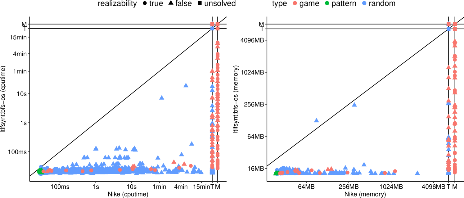
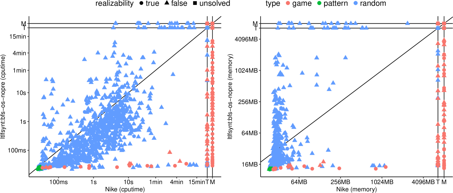
Figure 8 compare the best configuration of ltlfsynt against Nike: there are no cases where Nike is faster. If we disable preprocessings and one-step (un)realizability in ltlfsynt, the comparison is more balanced, as shown in Figure 8. Note that we have kept one-step (un)realizability enabled in this comparison, because Nike uses it too. This is the reason why pattern benchmarks are solved instantaneously by both tools.
Tables 2, 3, and 4 look at the runtime of the tools on game benchmarks. Values highlighted in yellow are within 5% of the minimum value of each line.
Table 2 shows a family of specifications where preprocessings are useless, and using one-step (un)realizability slows things down.
Table 3 shows a family of specifications where one-step (un)realizability is what allows ltlfsynt to solve many more instance than other tools (even tools like Nike or LydiaSyft who also implement one-step (un)realizability). The suspicious behavior of Lydia/LidyaSyft/SyftMax cycling between timeouts, segmentation faults, and out-of-memory has been double-checked: this is really how they terminated.
Finally, Table 4 shows very impressive results by ltlfsynt on the challenging Nim family of benchmarks: the highest configuration that third-party tools are able to solve is nim_04_01, but ltlfsynt solves this instantaneously in all configurations, and can handle much larger instances.
\includestandalonecounter-table
\includestandalonecounters-table
\includestandalonenim-table
A more detailed analysis of the benchmark results can be found in directory ltlfsynt-analysis/ of the associated artifact [24].