Enhanced curvature perturbations from spherical domain walls nucleated during inflation

Domain walls (DWs) are sheet-like topological defects in three spatial dimensions that can be generated in the early Universe when a discrete symmetry is spontaneously broken. A variety of new physics models predict the existance of DWs Zeldovich et al. (1974); Kibble (1976); Vilenkin (1981), such as axion models Linde and Lyth (1990); Sikivie (1982); Hiramatsu et al. (2013a); Cicoli et al. (2012); Arvanitaki et al. (2010), suppersymmetric models Dvali and Shifman (1997); Kovner et al. (1997); Takahashi et al. (2008); Dine et al. (2010), and the Standard model Higgs Buttazzo et al. (2013); Andreassen et al. (2014); Krajewski et al. (2016). DWs receive extensive investigation since the formation and evolution of DWs leave trace on various cosmological observations including the large-scale structure Vilenkin (1985a); Hill et al. (1989), the cosmic microwave background (CMB) Zeldovich et al. (1974); Takahashi and Yin (2021); Gonzalez et al. (2022), stochastic gravitational wave backgrounds (SGWBs) Hiramatsu et al. (2014); Saikawa (2017a); Hiramatsu et al. (2013b); Wei and Jiang (2022); Sakharov et al. (2021); Liu et al. (2021) and first-order phase transitions Blasi and Mariotti (2022).

The formation of the DW network was regarded as a disaster in cosmology Zeldovich et al. (1974); Vilenkin (1985b); Saikawa (2017b). The curvature radius of DWs is comparable to the Hubble horizon size and the proportion of two different vacua are comparable to each other, which is well-known as the scaling behavior of DWs Press et al. (1989); Hindmarsh (1996). Numerical results confirm that the DW energy density scales as $\rho_{DW}\propto t^{-1}$ in the matter-dominated (MD) and radiation-dominated (RD) eras Martins et al. (2016); Leite and Martins (2011); Leite et al. (2013). Since $\rho_{DW}$ decreases much slower than the energy density of radiation and matter, DWs will finally dominate the Universe which conflicts with the present observations Collaboration et al. (2020). The temperature fluctuations of the CMB imply that DWs with tension $\sigma>\mathcal{O}(\mathrm{MeV}^{3})$ does not exist in the Universe at pressent Zeldovich et al. (1974). In general, the DW problem can be avoided by introducing a bias term in the effective potential so that DWs become unstable. In this case, the DW tension and the annihilation time can be constrained by the SGWB produced from the DW network Hiramatsu et al. (2014); Saikawa (2017a), see Ref. Jiang and Huang (2022) and Refs. Bian et al. (2022); Ferreira et al. (2022) for corresponding constraints from LIGO-Virgo and pulsar timing array experiments. Ref. Ramberg et al. (2022) obtains the constraint on DWs from CMB spectral distortions.

In this work, we focus on spherical DWs nucleated through quantum tunneling during inflation Basu et al. (1991); Liu et al. (2020a). This scenario of DW formation and evolution is remarkably different from the scaling case. The radius of spherical DWs is comparable to the Hubble scale at the nucleation time. Once DWs are nucleated, they are stretched by inflation and remain stable at superhorizon scales. The Hubble horizon expands after inflation, and DWs begin to collapse when they reenter the Hubble horizon. Since the tunneling rate is exponentially suppressed by the Euclidean action of DWs, $S_{E}$, the DW problem is naturally avoided in this scenario. We consider the case that DWs have nonnegligible interaction with the matter fields so that the energy stored in DWs finally transforms into background radiation Vachaspati et al. (1984); Pujolas and Zahariade (2022); Blasi et al. (2022), rather than primordial black holes (PBHs) Tanahashi and Yoo (2015); Garriga et al. (2016); Deng et al. (2017a); Liu et al. (2020b); Ge (2020). According to Birkhoff’s theorem, the collapse of a single spherical DW cannot produce gravitational waves (GWs). However, the inhomogeneous distribution of spherical DWs induces curvature perturbations which can serve as the source of scalar-induced GWs, providing an opportunity to verify or give constraints to this scenario. Since the nucleation of different DWs is independent of each other, the statistics of DWs obey the Poisson distribution and induce superhorizon curvature perturbations with a typical $k^{3}$ slope in the infrared power spectrum. We obtain the energy spectrum of scalar-induced GWs which is expected to be detected in multiband GW detectors. For convenience, we choose $c=8\pi G=1$ throughout this paper.

Induced curvature perturbations reenter the Hubble horizon and begin to evolve soon after the annihilation of DWs. Since the collapse of a single spherical DW cannot produce GWs, the unique SGWB in this scenario is induced by curvature perturbations predicted in the last section. In this section, we introduce the formula to calculate GWs induced by scalar perturbations at the second order Espinosa et al. (2018); Kohri and Terada (2018). The perturbed metric of a Friedmann-Robertson-Walker Universe in the Newtonian gauge reads

	$\displaystyle ds^{2}$	$\displaystyle=$	$\displaystyle a^{2}(\tau)\Big{\{}-(1+2\Phi)d\tau^{2}$		(20)
			$\displaystyle+[(1-2\Psi)\delta_{ij}+\frac{1}{2}h_{ij}]dx^{i}dx^{j}\Big{\}},$

where $\tau$ is conformal time, $\Phi$ and $\Psi$ represent scalar perturbations and $h_{ij}$ denotes tensor perturbations of the second order. Here, we neglect vector perturbations and first-order tensor perturbations. We also neglect the anisotropic pressure so that we take $\Phi=\Psi$ in the following. The equation of motion (EoM) of the tensor modes sourced by curvature perturbations reads

$$h_{ij}^{\prime\prime}+2\mathcal{H}h_{ij}^{\prime}-\nabla^{2}h_{ij}=-4\Pi_{ij}^{lm}\mathcal{S}_{lm},$$

(21)

$\Pi_{ij}^{lm}$ is the transverse-traceless projection operator and $S_{lm}$ is the scalar-induced source term. Tensor perturbations can be expanded into the Fourier modes as

$$h_{ij}(\tau,\bm{x})=\int\frac{d^{3}k}{(2\pi)^{3/2}}\left[e_{ij}^{+}(\bm{k})h_{\bm{k}}^{+}+e_{ij}^{\times}(\bm{k})h_{\bm{k}}^{\times}\right]e^{i\bm{k}\cdot\bm{x}},$$

(22)

where $e_{ij}^{\lambda}(\bm{k})(\lambda=+,\times)$ are the polarization tensors. Similarly, the Fourier modes of the source term are

$$\Pi_{ij}^{lm}\mathcal{S}_{lm}(\tau,\bm{x})=\sum_{\lambda=+,\times}\int\frac{d^{3}k}{(2\pi)^{3/2}}e_{ij}^{\lambda}(\bm{k})e^{\lambda,lm}(\bm{k})S_{lm}(\tau,k)\,.$$

(23)

Then, the EoM of the tensor modes $h_{\bm{k}}(\tau)$ can be written in the form

$$h_{\bm{k}}^{\prime\prime}(\tau)+2\mathcal{H}h_{\bm{k}}^{\prime}(\tau)+k^{2}h_{\bm{k}}(\tau)=4S_{\bm{k}}(\tau)\,.$$

(24)

Here, we ignore the upper index of two different polarization modes since they satisfy the same equation. The source term $S_{\bm{k}}$ reads

	$\displaystyle S_{\bm{k}}(\tau)$	$\displaystyle=$	$\displaystyle\int\frac{d^{3}q}{(2\pi)^{3/2}}e_{ij}(\bm{k})q_{i}q_{j}\Bigg{[}2\Phi_{\bm{q}}\Phi_{\bm{k-q}}+\frac{4}{3(1+3\omega)}$		(25)
			$\displaystyle\times(\mathcal{H}^{-1}\Phi^{\prime}_{\bm{q}}+\Phi_{\bm{q}})(\mathcal{H}^{-1}\Phi^{\prime}_{\bm{k-q}}+\Phi_{\bm{k-q}})\Bigg{]}\,,$

where $\omega$ is the equation of state parameter of the Universe and $\omega=1/3$ in the RD era. The Newtonian potential $\Phi$ obeys the following equation

$$\Phi_{k}^{\prime\prime}+\frac{6(1+\omega)}{1+3\omega}\frac{1}{\tau}\Phi_{k}^{\prime}+\omega^{2}k^{2}\Phi_{k}=0\,,$$

(26)

where we ignore entropy perturbations. The initial value of the Newtonian potential, $\Phi_{k,0}$, is related to the power spectrum of curvature perturbations as

$$\left\langle\Phi_{k,0}\Phi_{k^{\prime},0}\right\rangle=\delta^{(3)}(\bm{k}-\bm{k^{\prime}})\frac{2\pi^{2}}{k^{3}}\left(\frac{3+3\omega}{5+3\omega}\right)^{2}{\cal P}_{\cal R}(k)\,.$$

(27)

We can use the Green’s function method to solve Eq. (24)

$$a(\tau)h_{\bm{k}}(\tau)=4\int^{\tau}d\tau_{1}\mathcal{G}(\tau,\tau_{1})a(\tau_{1})S_{\bm{k}}(\tau_{1})\,,$$

(28)

where the Green function $\mathcal{G}(\tau,\tau^{\prime})$ is the solution of

$$\mathcal{G}^{\prime\prime}_{\bm{k}}(\tau,\tau_{1})+\left(k^{2}-\frac{a^{\prime\prime}(\tau)}{a(\tau)}\right)\mathcal{G}_{\bm{k}}(\tau,\tau_{1})=\delta(\tau-\tau_{1})\,.$$

(29)

The power spectrum of tensor perturbations is defined by

$$\langle h_{\bm{k}}^{\lambda}(\tau)h_{\bm{k}^{\prime}}^{\lambda^{\prime}}(\tau)\rangle=\delta_{\lambda\lambda^{\prime}}\delta^{(3)}(\bm{k}-\bm{k}^{\prime})\frac{2\pi^{2}}{k^{3}}{\cal P}_{h}(\tau,k)\,.$$

(30)

The energy spectrum of GWs is defined as

$$\Omega_{\mathrm{GW}}(\tau,k)\equiv\frac{1}{\rho_{tot}}\frac{d\rho_{\mathrm{GW}}}{d\ln k}=\frac{1}{24}\left(\frac{k}{\mathcal{H}(\tau)}\right)^{2}\overline{{\cal P}_{h}(\tau,k)}\,,$$

(31)

where the overline represents the oscillation average and the two polarization modes have been added up. Then, in the RD era, $\Omega_{\mathrm{GW}}$ of scalar-induced GWs can be evaluated by the following integral

	$\displaystyle\Omega_{\mathrm{GW}}(\tau,k)$	$\displaystyle=$	$\displaystyle\frac{1}{12}\int_{0}^{\infty}dv\int_{|1-v|}^{|1+v|}du\left(\frac{4v^{2}-(1+v^{2}-u^{2})^{2}}{4uv}\right)^{2}$		(32)
			$\displaystyle\times{\cal P}_{\cal R}(ku){\cal P}_{\cal R}(kv)\left(\frac{3}{4u^{3}v^{3}}\right)^{2}(u^{2}+v^{2}-3)^{2}$
			$\displaystyle\times\Bigg{\{}\Bigg{[}-4uv+(u^{2}+v^{2}-3)\ln{\left|\frac{3-(u+v)^{2}}{3-(u-v)^{2}}\right|}\Bigg{]}^{2}$
			$\displaystyle+\pi^{2}(u^{2}+v^{2}-3)^{2}\Theta(u+v-\sqrt{3})\Bigg{\}}\,.$

In order to obtain the GW energy spectrum at present, we need to take the thermal history into consideration

$$\Omega_{\mathrm{GW}}(\tau_{0},k)=\Omega_{\gamma,0}\left(\frac{g_{*,0}}{g_{*,eq}}\right)^{\frac{1}{3}}\Omega_{\mathrm{GW}}(\tau_{eq},k)\,,$$

(33)

where $\Omega_{\gamma,0}$ is the density parameter of radiation at present, $g_{*,0}$ and $g_{*,eq}$ are the effect numbers of relativistic degrees of freedom at present and the radiation-matter equality, $\tau_{eq}$.

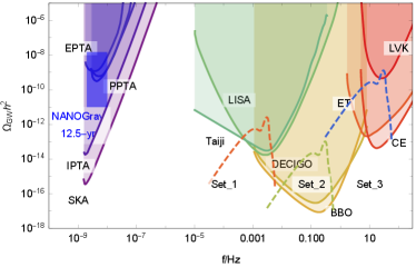
We choose three sets of parameters in Table. 1 to show the predictions of $\Omega_{\mathrm{GW}}$. The probability $p$, the abundance of DWs $\rho_{DW}/\rho_{r}$ and the cutoff scale $k_{cut}$ are determined by the DW tension $\sigma$ and the evolution of $S_{E}$ during inflation, and thus can also be treated as free parameters with the only constraint $\rho_{DW}/\rho_{r}<p$ to avoid the formation of PBHs. For the three parameter sets, the predicted $\Omega_{\mathrm{GW}}$ peak at $0.001$Hz, $0.1$Hz and $10$Hz, respectively, which are expected to be detected by multiband GW detectors, including LISA/Taiji (set 1), DECIGO/BBO (set 2), CE/ET and LIGO-Virgo-KAGRA collaboration (set 3), as shown in Fig. 1.

The observation of the CMB temperature anisotropies give strict constraints on primordial curvature perturbations ${\cal P}_{\cal R}(k)\approx 2\times 10^{-9}$ for $10^{-3}\,\mathrm{Mpc}^{-1}\lesssim k\lesssim 1\,\mathrm{Mpc}^{-1}$. At smaller scales, the observations of CMB spectral distortions, big-bang nucleosynthesis and ultracompact minihaloes also give constraints on ${\cal P}_{\cal R}(k)$ at the scales of $1\,\mathrm{Mpc}^{-1}\lesssim k\lesssim 10^{8}\,\mathrm{Mpc}^{-1}$ Emami and Smoot (2018); Gow et al. (2021). In the three parameter sets of Table. 1, the results of ${\cal P}_{\cal R}$ are orders of magnitude smaller than $10^{-10}$ at the scale $k\sim 3\times 10^{7}\,\mathrm{Mpc}^{-1}$ so that we safely avoid the constraints on ${\cal P}_{\cal R}(k)$ from the observations of the CMB spectrum distortion and the ultracompact minihalo abundance. However, because of the limit on ${\cal P}_{\cal R}(k)$, GWs are constrained to be $\Omega_{\mathrm{GW}}\lesssim 10^{-17}$ which is too weak to be observed in the nanohertz band by SKA.

We show the results of ${\cal P}_{\cal R}(k)$ and $\Omega_{\mathrm{GW}}$ of scalar-induced GWs in a realistic two-field inflationary model where $S_{E}$ changes with time during inflation. The action reads

$$S=\int d^{4}x\sqrt{-g}\left[-\frac{R}{2}+\frac{1}{2}\partial^{\mu}\phi\partial_{\mu}\phi+\frac{1}{2}\partial^{\mu}\chi\partial_{\mu}\chi+V(\phi,\chi)\right],$$

(34)

with the potential $V(\phi,\chi)$

$$V(\phi,\chi)=\frac{\lambda_{\chi}}{4}\left[\chi^{2}-\alpha^{2}(\phi-\phi_{c})^{2}-m^{2}\right]^{2}+f(\phi)\,,$$

(35)

which provides two degenerate vacua in the $\chi$ direction. Since the dynamics of $\phi$ is unaffected by $\chi$ during inflation, the term $f(\phi)$ alone is responsible for the inflationary dynamics and generating primordial perturbations Aghanim et al. (2020).

The Friedmann equation and the EoMs of $\phi$ and $\chi$ are

	$\displaystyle H^{2}=\frac{1}{3}\left[\frac{1}{2}\dot{\phi}^{2}+\frac{1}{2}\dot{\chi}^{2}+V(\phi,\chi)\right]\,,$
	$\displaystyle\ddot{\phi}+3H\dot{\phi}+\frac{\partial V}{\partial\phi}=0\,,$
	$\displaystyle\ddot{\chi}+3H\dot{\chi}+\frac{\partial V}{\partial\chi}=0\,.$		(36)

We consider Starobinsky inflation with the potential

$$f(\phi)=\Lambda_{0}\left(1-e^{-\sqrt{\frac{2}{3}}\phi}\right)^{2}\,.$$

(37)

The tension of DWs is a function of $\phi(t)$

$$\sigma_{\chi}(t)=\frac{4}{4}\sqrt{\frac{\lambda_{\chi}}{2}}\left[\alpha^{2}(\phi^{2}-\phi_{c}^{2})^{2}+m^{2}\right]^{\frac{3}{2}}.$$

(38)

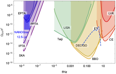
At the time $\phi(t)=\phi_{c}$, the Euclidean action $S_{E}=2\pi^{2}\sigma_{\chi}(t)H^{-3}(t)$ reaches minimum and most of DWs nucleate. We choose a specific parameter set to show the result of the energy spectrum of induced GWs in Fig. 2, where $\lambda_{\chi}=0.3,\alpha=1\times 10^{-5},\phi_{c}=3.9,m=5\times 10^{-6}$. The initial value of the scalar fields are set to be $\phi_{i}=5.1$and $\chi_{i}=0.0008$ so that the predicted $e$-folds is $N=50$. $\Omega_{\mathrm{GW}}$ peaks at about $1$Hz with the peak value $\sim 10^{-10}$, which is expected to be observed by DECIGO and BBO.

We have investigated spherical DWs nucleated during inflation via quantum tunneling and found their random distribution induces curvature perturbations at the length scales larger than the mean separation of spherical DWs. The statistics of DWs turn out to be the Poisson type and the power spectrum of induced curvature perturbations is proportional to $k^{3}$. We numerically calculate the energy spectrum of scalar-induced GWs in terms of ${\cal P}_{\cal R}(k)$ which can be detected by multiband GW detectors. Since the collapse of spherical DWs does not directly produce GWs, our work provides a practical method to detect or constrain the case that the energy of spherical DWs decays into radiation.

This result is also applicable to false vacuum bubbles nucleated during inflation, proposed in Refs. Ashoorioon (2015); Ashoorioon et al. (2021); Deng and Vilenkin (2017); Deng (2020), where the vacua of the effective potential are nondegenerate. Induced curvature perturbations from Poisson distribution have been also discussed in other physical processes in the early Universe such as PBH formation Papanikolaou et al. (2021, 2022); Bhaumik et al. (2022a, b); Domènech et al. (2021) and first-order phase transitions Liu et al. (2022). These processes directly produce another SGWB from the transverse-traceless part of the energy-momentum tensor, which could be distinguished from the random distribution of spherical DWs or false vacuum bubbles.

This work is supported in part by the National Key Research and Development Program of China Grant No.2020YFC2201501, in part by the National Natural Science Foundation of China Grants No. 12105060, No. 12147103, No. 12075297 and No. 12235019, and in part by the Fundamental Research Funds for the Central Universities.

References

- Zeldovich et al. (1974) Y. B. Zeldovich, I. Y. Kobzarev, and L. B. Okun, Zh. Eksp. Teor. Fiz. 67, 3 (1974).
- Kibble (1976) T. W. B. Kibble, Journal of Physics A: Mathematical and General 9, 1387 (1976).
- Vilenkin (1981) A. Vilenkin, Phys. Rev. D 23, 852 (1981).
- Linde and Lyth (1990) A. D. Linde and D. H. Lyth, Physics Letters B 246, 353 (1990).
- Sikivie (1982) P. Sikivie, Phys. Rev. Lett. 48, 1156 (1982).
- Hiramatsu et al. (2013a) T. Hiramatsu, M. Kawasaki, K. Saikawa, and T. Sekiguchi, JCAP 01, 001, arXiv:1207.3166 [hep-ph] .
- Cicoli et al. (2012) M. Cicoli, M. Goodsell, and A. Ringwald, JHEP 10, 146, arXiv:1206.0819 [hep-th] .
- Arvanitaki et al. (2010) A. Arvanitaki, S. Dimopoulos, S. Dubovsky, N. Kaloper, and J. March-Russell, Phys. Rev. D 81, 123530 (2010), arXiv:0905.4720 [hep-th] .
- Dvali and Shifman (1997) G. R. Dvali and M. A. Shifman, Phys. Lett. B 396, 64 (1997), [Erratum: Phys.Lett.B 407, 452 (1997)], arXiv:hep-th/9612128 .
- Kovner et al. (1997) A. Kovner, M. A. Shifman, and A. V. Smilga, Phys. Rev. D 56, 7978 (1997), arXiv:hep-th/9706089 .
- Takahashi et al. (2008) F. Takahashi, T. T. Yanagida, and K. Yonekura, Physics Letters B 664, 194 (2008).
- Dine et al. (2010) M. Dine, F. Takahashi, and T. T. Yanagida, JHEP 07, 003, arXiv:1005.3613 [hep-th] .
- Buttazzo et al. (2013) D. Buttazzo, G. Degrassi, P. P. Giardino, G. F. Giudice, F. Sala, A. Salvio, and A. Strumia, JHEP 12, 089, arXiv:1307.3536 [hep-ph] .
- Andreassen et al. (2014) A. Andreassen, W. Frost, and M. D. Schwartz, Phys. Rev. Lett. 113, 241801 (2014), arXiv:1408.0292 [hep-ph] .
- Krajewski et al. (2016) T. Krajewski, Z. Lalak, M. Lewicki, and P. Olszewski, JCAP 12, 036, arXiv:1608.05719 [astro-ph.CO] .
- Vilenkin (1985a) A. Vilenkin, Phys. Rept. 121, 263 (1985a).
- Hill et al. (1989) C. T. Hill, D. N. Schramm, and J. N. Fry, Comments Nucl. Part. Phys. 19, 25 (1989).
- Takahashi and Yin (2021) F. Takahashi and W. Yin, JCAP 04, 007, arXiv:2012.11576 [hep-ph] .
- Gonzalez et al. (2022) D. Gonzalez, N. Kitajima, F. Takahashi, and W. Yin, (2022), arXiv:2211.06849 [hep-ph] .
- Hiramatsu et al. (2014) T. Hiramatsu, M. Kawasaki, and K. Saikawa, JCAP 02, 031, arXiv:1309.5001 [astro-ph.CO] .
- Saikawa (2017a) K. Saikawa, Universe 3, 40 (2017a), arXiv:1703.02576 [hep-ph] .
- Hiramatsu et al. (2013b) T. Hiramatsu, M. Kawasaki, K. Saikawa, and T. Sekiguchi, Journal of Cosmology and Astroparticle Physics 2013 (01), 001, arXiv:1207.3166 [astro-ph, physics:hep-ph].
- Wei and Jiang (2022) D. Wei and Y. Jiang, (2022), arXiv:2208.07186 [hep-ph] .
- Sakharov et al. (2021) A. S. Sakharov, Y. N. Eroshenko, and S. G. Rubin, Phys. Rev. D 104, 043005 (2021).
- Liu et al. (2021) J. Liu, R.-G. Cai, and Z.-K. Guo, Phys. Rev. Lett. 126, 141303 (2021), arXiv:2010.03225 [astro-ph.CO] .
- Blasi and Mariotti (2022) S. Blasi and A. Mariotti, Phys. Rev. Lett. 129, 261303 (2022), arXiv:2203.16450 [hep-ph] .
- Vilenkin (1985b) A. Vilenkin, Physics Reports 121, 263 (1985b).
- Saikawa (2017b) K. Saikawa, Universe 3, 40 (2017b), arXiv:1703.02576 [astro-ph, physics:gr-qc, physics:hep-ph].
- Press et al. (1989) W. H. Press, B. S. Ryden, and D. N. Spergel, Astrophys. J. 347, 590 (1989).
- Hindmarsh (1996) M. Hindmarsh, Physical Review Letters 77, 4495 (1996), arXiv:hep-ph/9605332.
- Martins et al. (2016) C. J. A. P. Martins, I. Y. Rybak, A. Avgoustidis, and E. P. S. Shellard, Physical Review D 93, 043534 (2016), arXiv:1602.01322 [astro-ph, physics:gr-qc, physics:hep-ph, physics:hep-th].
- Leite and Martins (2011) A. M. M. Leite and C. J. A. P. Martins, Physical Review D 84, 103523 (2011), arXiv:1110.3486 [astro-ph, physics:hep-ph, physics:hep-th].
- Leite et al. (2013) A. M. M. Leite, C. J. A. P. Martins, and E. P. S. Shellard, Physics Letters B 718, 740 (2013), arXiv:1206.6043 [hep-ph, physics:hep-th].
- Collaboration et al. (2020) P. Collaboration, Y. Akrami, and et al, Astronomy & Astrophysics 641, A1 (2020), arXiv: 1807.06205.
- Jiang and Huang (2022) Y. Jiang and Q.-G. Huang, Phys. Rev. D 106, 103036 (2022), arXiv:2208.00697 [astro-ph.CO] .
- Bian et al. (2022) L. Bian, S. Ge, C. Li, J. Shu, and J. Zong, (2022), arXiv:2212.07871 [hep-ph] .
- Ferreira et al. (2022) R. Z. Ferreira, A. Notari, O. Pujolas, and F. Rompineve, (2022), arXiv:2204.04228 [astro-ph.CO] .
- Ramberg et al. (2022) N. Ramberg, W. Ratzinger, and P. Schwaller, (2022), arXiv:2209.14313 [hep-ph] .
- Basu et al. (1991) R. Basu, A. H. Guth, and A. Vilenkin, Physical Review D 44, 340 (1991).
- Liu et al. (2020a) J. Liu, Z.-K. Guo, and R.-G. Cai, Physical Review D 101, 023513 (2020a), arXiv:1908.02662 [astro-ph, physics:gr-qc, physics:hep-th].
- Vachaspati et al. (1984) T. Vachaspati, A. E. Everett, and A. Vilenkin, Phys. Rev. D 30, 2046 (1984).
- Pujolas and Zahariade (2022) O. Pujolas and G. Zahariade, (2022), arXiv:2212.11204 [hep-th] .
- Blasi et al. (2022) S. Blasi, A. Mariotti, A. Rase, A. Sevrin, and K. Turbang, (2022), arXiv:2210.14246 [hep-ph] .
- Tanahashi and Yoo (2015) N. Tanahashi and C.-M. Yoo, Class. Quant. Grav. 32, 155003 (2015), arXiv:1411.7479 [gr-qc] .
- Garriga et al. (2016) J. Garriga, A. Vilenkin, and J. Zhang, JCAP 02, 064, arXiv:1512.01819 [hep-th] .
- Deng et al. (2017a) H. Deng, J. Garriga, and A. Vilenkin, JCAP 04, 050, arXiv:1612.03753 [gr-qc] .
- Liu et al. (2020b) J. Liu, Z.-K. Guo, and R.-G. Cai, Phys. Rev. D 101, 023513 (2020b), arXiv:1908.02662 [astro-ph.CO] .
- Ge (2020) S. Ge, Phys. Dark Univ. 27, 100440 (2020), arXiv:1905.12182 [hep-ph] .
- Garriga (1994) J. Garriga, Physical Review D 49, 6327 (1994), arXiv:hep-ph/9308280.
- Bardeen et al. (1986) J. M. Bardeen, J. R. Bond, N. Kaiser, and A. S. Szalay, Astrophys. J. 304, 15 (1986).
- Deng et al. (2017b) H. Deng, J. Garriga, and A. Vilenkin, Journal of Cosmology and Astroparticle Physics 2017 (04), 050, arXiv:1612.03753 [gr-qc, physics:hep-th].
- Espinosa et al. (2018) J. R. Espinosa, D. Racco, and A. Riotto, JCAP 09, 012, arXiv:1804.07732 [hep-ph] .
- Kohri and Terada (2018) K. Kohri and T. Terada, Phys. Rev. D 97, 123532 (2018), arXiv:1804.08577 [gr-qc] .
- Emami and Smoot (2018) R. Emami and G. Smoot, JCAP 01, 007, arXiv:1705.09924 [astro-ph.CO] .
- Gow et al. (2021) A. D. Gow, C. T. Byrnes, P. S. Cole, and S. Young, JCAP 02, 002, arXiv:2008.03289 [astro-ph.CO] .
- Lentati et al. (2015) L. Lentati et al., Mon. Not. Roy. Astron. Soc. 453, 2576 (2015), arXiv:1504.03692 [astro-ph.CO] .
- Shannon et al. (2015) R. M. Shannon et al., Science 349, 1522 (2015), arXiv:1509.07320 [astro-ph.CO] .
- Arzoumanian et al. (2018) Z. Arzoumanian et al. (NANOGRAV), Astrophys. J. 859, 47 (2018), arXiv:1801.02617 [astro-ph.HE] .
- Arzoumanian et al. (2020) Z. Arzoumanian et al. (NANOGrav), Astrophys. J. Lett. 905, L34 (2020), arXiv:2009.04496 [astro-ph.HE] .
- Hobbs et al. (2010) G. Hobbs et al., Gravitational waves. Proceedings, 8th Edoardo Amaldi Conference, Amaldi 8, New York, USA, June 22-26, 2009, Class. Quant. Grav. 27, 084013 (2010), arXiv:0911.5206 [astro-ph.SR] .
- Carilli and Rawlings (2004) C. L. Carilli and S. Rawlings, International SKA Conference 2003 Geraldton, Australia, July 27-August 2, 2003, New Astron. Rev. 48, 979 (2004), arXiv:astro-ph/0409274 [astro-ph] .
- Amaro-Seoane et al. (2017) P. Amaro-Seoane et al. (LISA), (2017), arXiv:1702.00786 [astro-ph.IM] .
- Ruan et al. (2018) W.-H. Ruan, Z.-K. Guo, R.-G. Cai, and Y.-Z. Zhang, (2018), arXiv:1807.09495 [gr-qc] .
- Kawamura et al. (2011) S. Kawamura et al., Laser interferometer space antenna. Proceedings, 8th International LISA Symposium, Stanford, USA, June 28-July 2, 2010, Class. Quant. Grav. 28, 094011 (2011).
- Phinney et al. (2004) S. Phinney, P. Bender, R. Buchman, R. Byer, N. Cornish, P. Fritschel, W. Folkner, S. Merkowitz, K. Danzmann, L. DiFiore, et al., NASA Mission Concept Study (2004).
- Aasi et al. (2015) J. Aasi et al. (LIGO Scientific), Class. Quant. Grav. 32, 074001 (2015), arXiv:1411.4547 [gr-qc] .
- Somiya (2012) K. Somiya (KAGRA), Gravitational waves. Numerical relativity - data analysis. Proceedings, 9th Edoardo Amaldi Conference, Amaldi 9, and meeting, NRDA 2011, Cardiff, UK, July 10-15, 2011, Class. Quant. Grav. 29, 124007 (2012), arXiv:1111.7185 [gr-qc] .
- Reitze et al. (2019) D. Reitze et al., Bull. Am. Astron. Soc. 51, 035 (2019), arXiv:1907.04833 [astro-ph.IM] .
- Punturo et al. (2010) M. Punturo et al., Proceedings, 14th Workshop on Gravitational wave data analysis (GWDAW-14): Rome, Italy, January 26-29, 2010, Class. Quant. Grav. 27, 194002 (2010).
- Schmitz (2021) K. Schmitz, JHEP 01, 097, arXiv:2002.04615 [hep-ph] .
- Aghanim et al. (2020) N. Aghanim et al. (Planck), Astron. Astrophys. 641, A6 (2020), [Erratum: Astron.Astrophys. 652, C4 (2021)], arXiv:1807.06209 [astro-ph.CO] .
- Ashoorioon (2015) A. Ashoorioon, Phys. Lett. B 747, 446 (2015), arXiv:1502.00556 [astro-ph.CO] .
- Ashoorioon et al. (2021) A. Ashoorioon, A. Rostami, and J. T. Firouzjaee, Phys. Rev. D 103, 123512 (2021), arXiv:2012.02817 [astro-ph.CO] .
- Deng and Vilenkin (2017) H. Deng and A. Vilenkin, JCAP 12, 044, arXiv:1710.02865 [gr-qc] .
- Deng (2020) H. Deng, JCAP 09, 023, arXiv:2006.11907 [astro-ph.CO] .
- Papanikolaou et al. (2021) T. Papanikolaou, V. Vennin, and D. Langlois, JCAP 03, 053, arXiv:2010.11573 [astro-ph.CO] .
- Papanikolaou et al. (2022) T. Papanikolaou, C. Tzerefos, S. Basilakos, and E. N. Saridakis, JCAP 10, 013, arXiv:2112.15059 [astro-ph.CO] .
- Bhaumik et al. (2022a) N. Bhaumik, A. Ghoshal, and M. Lewicki, JHEP 07, 130, arXiv:2205.06260 [astro-ph.CO] .
- Bhaumik et al. (2022b) N. Bhaumik, A. Ghoshal, R. K. Jain, and M. Lewicki, (2022b), arXiv:2212.00775 [astro-ph.CO] .
- Domènech et al. (2021) G. Domènech, C. Lin, and M. Sasaki, JCAP 04, 062, [Erratum: JCAP 11, E01 (2021)], arXiv:2012.08151 [gr-qc] .
- Liu et al. (2022) J. Liu, L. Bian, R.-G. Cai, Z.-K. Guo, and S.-J. Wang, (2022), arXiv:2208.14086 [astro-ph.CO] .