[table]capposition=top \newfloatcommandcapbtabboxtable[][\FBwidth]
Enhancing Semi-Supervised Learning via Representative and Diverse Sample Selection
Abstract
Semi-Supervised Learning (SSL) has become a preferred paradigm in many deep learning tasks, which reduces the need for human labor. Previous studies primarily focus on effectively utilising the labelled and unlabeled data to improve performance. However, we observe that how to select samples for labelling also significantly impacts performance, particularly under extremely low-budget settings. The sample selection task in SSL has been under-explored for a long time. To fill in this gap, we propose a Representative and Diverse Sample Selection approach (RDSS). By adopting a modified Frank-Wolfe algorithm to minimise a novel criterion -Maximum Mean Discrepancy (-MMD), RDSS samples a representative and diverse subset for annotation from the unlabeled data. We demonstrate that minimizing -MMD enhances the generalization ability of low-budget learning. Experimental results show that RDSS consistently improves the performance of several popular SSL frameworks and outperforms the state-of-the-art sample selection approaches used in Active Learning (AL) and Semi-Supervised Active Learning (SSAL), even with constrained annotation budgets. Our code is available at RDSS.
1 Introduction
Semi-Supervised Learning (SSL) is a popular paradigm which reduces reliance on large amounts of labeled data in many deep learning tasks [40, 35, 59]. Previous SSL research mainly focuses on effectively utilising labelled and unlabeled data. Specifically, labelled data directly supervise model learning, while unlabeled data help learn a desirable model that makes consistent and unambiguous predictions [53]. Besides, we also find that how to select samples for annotation will greatly affect model performance, particularly under extremely low-budget settings (see Section 7.2).
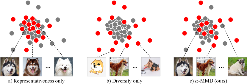
The prevailing sample selection methods in SSL have many shortcomings. For example, random sampling may introduce imbalanced class distributions and inadequate coverage of the overall data distribution, resulting in poor performance. Stratified sampling randomly selects samples within each class, which is impractical in real-world scenarios where the label for each sample is unknown. Existing researchers also employ representativeness and diversity strategies to select appropriate samples for annotation. Representativeness [13] ensures that the selected subset distributes similarly with the entire dataset, and diversity [54] is designed to select informative samples by pushing away them in feature space. And focusing on only one aspect presents significant limitations (Figure 1a and b). To address these issues, Xie et al. [57] and Wang et al. [50] employ a combination of the two strategies for sample selection. These methods set a fixed ratio for representativeness and diversity, restricting the ultimate performance through our empirical evidence (see Section 7.4). Fundamentally, they lack a theoretical basis to substantiate their effectiveness.
We observe that Active Learning (AL) primarily focuses on selecting the right samples for annotation, and numerous studies transfer the sample selection methods of AL into SSL, giving rise to Semi-Supervised Active Learning (SSAL) [51]. However, most of these approaches exhibit several limitations: (1) They require randomly selected samples to begin with, which expends a portion of the labelling budget, making it difficult to work effectively with a very limited budget (e.g., 1% or even lower) [6]; (2) They involve human annotators in iterative cycles of labelling and training, leading to substantial labelling overhead [57]; (3) They are coupled with the model training so that samples for annotation need to be re-selected every time a model is trained [50]. In summary, selecting the appropriate samples for annotation is challenging in SSL.
To address these challenges, we propose a Representative and Diverse Sample Selection approach (RDSS) that requests annotations only once and operates independently of the downstream tasks. Specifically, inspired by the concept of Maximum Mean Discrepancy (MMD) [14], we design a novel criterion named -MMD. It aims to strike a balance between representativeness and diversity via a trade-off parameter (Figure 1c), for which we find an optimal interval adapt to different budgets. By using a modified Frank-Wolfe algorithm called Generalized Kernel Herding without Replacement (GKHR), we can get an efficient approximate solution to this minimization problem.
We prove that under certain Reproducing Kernel Hilbert Space (RKHS) assumptions, -MMD effectively bounds the difference between training with a constrained versus an unlimited labelling budget. This implies that our proposed method could significantly enhance the generalization ability of learning with limited labels. We also give a theoretical assessment of GKHR with some supplementary numerical experiments, showing that GKHR performs well in learning with limited labels.
Furthermore, we evaluate our proposed RDSS across several popular SSL frameworks on the datasets CIFAR-10/100 [19], SVHN [30], STL-10 [9] and ImageNet [10]. Extensive experiments show that RDSS outperforms other sample selection methods widely used in SSL, AL or SSAL, especially with a constrained annotation budget. Besides, ablation experimental results demonstrate that RDSS outperforms methods using a fixed ratio.
The main contributions of this article are as follows:
-
•
We propose RDSS, which selects representative and diverse samples for annotation to enhance SSL by minimizing a novel criterion -MMD. Under low-budget settings, we develop a fast and efficient algorithm, GKHR, for optimization.
-
•
We prove that our method benefits the generalizability of the trained model under certain assumptions and rigorously establish an optimal interval for the trade-off parameter adapt to the different budgets.
-
•
We compare RDSS with sample selection strategies widely used in SSL, AL or SSAL, the results of which demonstrate superior sample efficiency compared to these strategies. In addition, we conduct ablation experiments to verify our method’s superiority over the fixed-ratio approach.
2 Related Work
Semi-Supervised Learning
Semi-Supervised Learning (SSL) effectively utilizes sparse labeled data and abundant unlabeled data for model training. Consistency Regularization [34, 20, 45], Pseudo-Labeling [21, 56] and their hybrid strategies [40, 63, 35] are commonly used in SSL. Consistency Regularization ensures the model’s output stays stable even when there’s noise or small changes in the input, usually from the data augmentation [55]. Pseudo-labelling integrates high-confidence data pseudo-labels directly into training, adhering to entropy minimization [23]. Moreover, an integrative approach that combines the aforementioned strategies can also achieve substantial results [53, 59]. Even though these approaches have been proven effective, they usually assume that labelled samples are randomly selected from each class (i.e., stratified sampling), which is not practical in real-world scenarios where the label for each sample is unknown.
Active Learning
Active learning (AL) aims to optimize the learning process by selecting the appropriate samples for labelling, reducing reliance on large labelled datasets. There are two different criteria for sample selection: uncertainty and representativeness. Uncertainty sampling selects samples about which the current model is most uncertain. Earlier studies utilized posterior probability [22, 49], entropy [18, 26], and classification margin [47] to estimate uncertainty. Recent research regards uncertainty as training loss [17, 60], influence on model performance [11, 24] or the prediction discrepancies between multiple classifiers [8]. However, uncertainty sampling methods may exhibit performance disparities across different models, leading researchers to focus on representativeness sampling, which aims to align the distribution of selected subset with that of the entire dataset [36, 39, 27]. Most AL approaches are difficult to perform well under extremely low-label settings. This may be because they usually require randomly selected samples to begin with and involve human annotators in iterative cycles of labelling and training, leading to substantial labelling overhead.
Model-Free Subsampling
Subsampling is a statistical approach which selects a subset with size as a surrogate for the full dataset with size . While model-based subsampling methods depend heavily on the model assumptions [1, 61], improper choice of the model could lead to bad performance of estimation and prediction. In that case, model-free subsampling is preferred in data-driven modelling tasks, as it does not depend on the model assumptions. There are mainly two kinds of popular model-free subsampling methods. The one is induced by minimizing statistical discrepancies, which forces the distribution of subset to be similar to that of full data, in other words, selects representative subsamples, such as Wasserstein distance [13], energy distance [28], uniform design [65], maximum mean discrepancy [7] and generalized empirical -discrepancy [66]. The other tends to select a diverse subset containing as many informative samples as possible [54]. The above-mentioned methodologies either exclusively focus on representativeness or diversity, which are difficult to effectively apply to SSL.
3 Problem Setup
Let be the unlabeled data space, be the label space, be the full unlabeled dataset and be an index set contained in , our goal is to find an index set such that the selected set of samples is the most informative. After that, we can get access to the true labels of selected samples and use the set of labelled data and the rest of the unlabeled data to train a deep learning model.
Following the methodology of previous works, we use representativeness and diversity as criteria for evaluating the informativeness of selected samples. Representativeness ensures the selected samples distribute similarly to the full unlabeled dataset. Diversity is proposed to prevent an excessive concentration of selected samples in high-density areas of the full unlabeled dataset. Furthermore, the cluster assumption in SSL suggests that the data tend to form discrete clusters, in which boundary points are likely to be located in the low-density area. Therefore, under this assumption, selected samples with diversity contain more boundary points than the non-diversified ones, which is desired in training classifiers.
As a result, our goal can be formulated by solving the following problem:
| (1) |
where and quantify the representativeness and diversity of selected samples respectively and is a hyperparameter to balance the trade-off representativeness and diversity.
Besides, we propose another two fundamental settings which are beneficial to the implementation of the framework: (1) Low-budget learning. The budget for many of the real-world tasks which require sample selection procedures is relatively low compared to the size of unlabeled data. Therefore, we set in default in the following context, including the analysis of the sampling algorithm and the experiments; (2) Sampling without Replacement. Compared with the setting of sampling with replacement, sampling without replacement offers several benefits which better match our tasks, including bias and variance reduction, precision increase and representativeness enhancement [25, 46].
4 Representative and Diversity Sample Selection
The Representative and Diverse Sample Selection (RDSS) framework consists of two steps: (1) Quantification. We quantify the representativeness and diversity of selected samples by a novel concept called -MMD (6), where is replaced by as the trade-off hyperparameter; (2) Optimization. We optimize -MMD by GKHR algorithm to obtain the optimally selected samples .
4.1 Quantification of Diversity and Representativeness
In classical statistics and machine learning problems, the inner product of data points , defined by , is employed to as a similarity measure between . However, the application of linear functions can be very restrictive in real-world problems. In contrast, kernel methods use kernel functions , including Gaussian kernels (RBF), Laplacian kernels and polynomial kernels, as non-linear similarity measures between , which are actually inner products of the projections of in some high-dimensional feature space [29].
Let be a kernel function on , and we employ to measure the similarity between any two points and the average similarity, denoted by
| (2) |
to measure the similarity between the selected samples. Obviously, can evaluate the diversity of since larger similarity implies smaller diversity.
As a statistical discrepancy which measures the distance between distributions, the maximum mean discrepancy (MMD) is introduced here to quantify the representativeness of to . Proposed by Gretton et al. [14], MMD is formally defined below:
Definition 4.1 (Maximum Mean Discrepancy).
Let be two Borel probability measures on . Suppose is sampled from the unit ball in a reproducing kernel Hilbert space (RKHS) associated with its reproducing kernel , i.e., , then the MMD between and is defined by
| (3) |
where and are independent copies.
We can next derive the empirical version for MMD that is able to measure the representativeness of relative to by replacing with the empirical distribution constructed by in (3):
| (4) |
Optimization objective. Set and in (1), where is a proper kernel function, our optimization objective becomes
| (5) |
Set , since is a constant, the objective function in (5) can be rewritten by
| (6) | ||||
which defines a new concept called -MMD, denoted by . This new concept distinguishes our method from those existing methods, which is essential for developing the sampling algorithms and theoretical analysis. Note that -MMD degenerates to classical MMD when and degenerates to average similarity when . As decreases, increases, thereby encouraging the diversity for sample selection.
Remark 1. In the following context, all the kernels are assumed to be characteristic and positive definite if not specified. The following illustrates the advantages of the two properties.
Characteristics kernels. The MMD is generally a pseudo-metric on the space of all Borel probability distributions, implying that the MMD between two different distributions can be zero. Nevertheless, MMD becomes a proper metric when is a characteristic kernel, i.e., for any Borel probability distribution on [29]. Therefore, MMD induced by characteristic kernels can be more appropriate for measuring representativeness.
Positive definite kernels. Aronszajn [2] showed that for every positive definite kernel , i.e., its Gram matrix is always positive definite and symmetric, it uniquely determines an RKHS and vice versa. This property is not only important for evaluating the property of MMD [43] but also required in optimizing MMD [32] by Frank-Wolfe algorithm.
4.2 Sampling Algorithm
In the previous research [36, 27, 50, 38, 58], sample selection is usually modelled by a non-convex combinatorial optimization problem. In contrast, following the idea of [4], we regard as a convex optimization problem by exploiting the convexity of -MMD, and then solve it by a fast iterative minimization procedure derived from Frank-Wolfe algorithm (see Appendix A for derivation details):
| (7) |
where . As an extension of kernel herding [7], its corresponding algorithm (see Algorithm 2) is called Generalized Kernel Herding (GKH). Note that is iteratively updated in Algorithm 2, which can save a lot of running time. However, GKH can select repeated samples that contradict the setting of sampling without replacement. To address this issue, we propose a modified iterating formula based on (7):
| (8) |
which admits no repetitiveness in the selected samples. Its corresponding algorithm (see Algorithm 1) is thereby named as Generalized Kernel Herding without Replacement (GKHR), employed as the sampling algorithm for RDSS.
Computational complexity. Despite the time cost for calculating kernel functions, the computational complexity of GKHR is , since in each iteration, the steps in lines 4 and 5 of Algorithm 2 respectively require computations. Note that GKH has the same order of computational complexity as GKHR.
5 Theoretical Analysis
5.1 Generalization Bounds
Recall the core-set approach in [36], i.e., for any ,
where is the full labeled dataset and is the core set, is the expected risk of , are empirical risk of on . The first term is unknown before we label the selected samples, and the second term can be upper bounded by the so-called generalization bounds [3, 64] which do not depend on the choice of core set. Therefore, to control the upper bound of , we only need to analyse the upper bound of the third term called core-set loss, which requires several mild assumptions. Shalit, et al. [37] derived a MMD-type upper bound for to estimate individual treatment effect, while our bound is generalized to a wider range of tasks.
Let be a hypothesis set in which we are going to select a predictor and suppose that the labelled data are i.i.d. sampled from a random vector defined on . We firstly assume that is an RKHS, which is mild in machine learning theory [3, 5].
Assumption 5.1.
is an RKHS associated with bounded positive definite kernel where the norm of any is bounded by .
We further make RKHS assumptions on the functional space of and that are fundamental in the field of conditional distribution embedding [41, 43].
Assumption 5.2.
There is an RKHS associated with bounded positive definite kernel such that and the norm of any is bounded by .
Assumption 5.3.
There is an RKHS associated with bounded positive definite kernel such that and the norm of any is bounded by .
We next give a -MMD-type upper bound for the core-set loss by the following theorem:
Theorem 5.4.
Take , then under assumptions 1-3, for any selected samples , there exists a positive constant such that the following inequality holds:
where , and are projections of on .
Therefore, minimizing -MMD can optimize the generalization bound for and benefit the generalizability of the trained model (predictor).
5.2 Finite-Sample-Error-Bound for GKHR
The concept of convergence does not apply to analyzing GKHR. With fixed, GKHR iterates for at most times and then returns . Consequently, we analyze the performance of GKHR by its finite-sample-error bound. Previous to that, we make an assumption on the mean of over the full unlabeled dataset.
Assumption 5.5.
For any returned by GKHR, , there exists elements in such that
When is not relatively small, this assumption is rather unrealistic. Nevertheless, under our low-budget setting, especially when , the assumption becomes an extension of the principle that "the minimum is never larger than the mean", which still probably makes sense. We can then show that the decaying rate for optimization error of GKHR can be upper bounded by :
Theorem 5.6.
Let be the samples selected by GKHR, under assumption 4, it holds that
| (9) |
where , , where is defined in Lemma B.6.
6 Choice of Kernel and Hyperparameter Tuning
In this section, we make some suggestions for choosing the kernel and tuning the hyperparameter .
Choice of kernel. Recall Remark 1 in Section 4.1, we only consider characteristic and positive definite kernels in RDSS. Since the Gaussian kernels are the most commonly used kernels in the field of machine learning and statistics [3, 15], we introduce Gaussian kernel as our choice, which is defined by . The bandwidth parameter is set to be the median distance between samples in the aggregate dataset [15], i.e., , since the median is robust and also compromises between extreme cases.
Tuning trade-off hyperparameter . According to Theorem 5.6 and Lemma B.3, by straightforward deduction we have
to upper bound the MMD between the selected samples and the full dataset under a low-budget setting. We can just set so that the upper bound of the MMD would not be larger than the one of -MMD in the perspective of the order of magnitude.
7 Experiments
In this section, we first explain the implementation details of our method RDSS in Section 7.1. Next, we compare RDSS with other sampling methods by integrating them into two state-of-the-art (SOTA) SSL approaches (FlexMatch [63] and Freematch [53]) on five datasets (CIFAR-10/100, SVHN, STL-10 and ImageNet-1k) in Section 7.2. The details of the datasets, the visualization results and the computational complexity of different sampling methods are shown in Appendix D.2, D.3, and D.4, respectively. We also compare against various AL/SSAL approaches in Section 7.3. Lastly, we make quantitative analyses of the trade-off parameter in Section 7.4.
7.1 Implementation Details of Our Method
First, we leverage the pre-trained image feature extraction capabilities of CLIP [33], a vision transformer architecture, to extract features. Subsequently, the [CLS] token features produced by the model’s final output are employed for sample selection. During the sample selection phase, the Gaussian kernel function is chosen as the kernel method to compute the similarity of samples in an infinite-dimensional feature space. The value of for the Gaussian kernel function is set as explained in Section 6. To ensure diversity in the sampled data, we introduce a penalty factor given by , where denotes the number of selected samples. Concretely, we set for CIFAR-10, for CIFAR-100, for SVHN, for STL-10 and for ImageNet. Next, the selected samples are used for two SSL approaches, which are trained and evaluated on the datasets using the codebase Unified SSL Benchmark (USB) [52]. The optimizer for all experiments is standard stochastic gradient descent (SGD) with a momentum of [44]. The initial learning rate is with a learning rate decay of . We use ResNet-50 [16] for the ImageNet experiment and Wide ResNet-28-2 [62] for other datasets. Finally, we evaluate the performance with the Top-1 classification accuracy metric on the test set. Experiments are run on 8*NVIDIA Tesla A100 (40 GB) and 2*Intel 6248R 24-Core Processor. We average our results over five independent runs.
7.2 Comparison with Other Sampling Methods
Main results We apply RDSS on Flexmatch and Freematch to compare with the following three baselines and two SOTA methods in SSL under different annotation budget settings. The baselines conclude Stratified, Random and -Means, while the two SOTA methods are USL [50] and ActiveFT [57]. The results are shown on Table 1 from which we have several observations: (1) Our proposed RDSS achieves the highest accuracy, outperforming other sampling methods, which underscores the effectiveness of our approach; (2) USL attains suboptimal results under most budget settings yet exhibits a significant gap compared to RDSS, particularly under severely constrained ones. For instance, FreeMatch achieves a rise on the STL-10 with a budget of ; (3) In most experiments, RDSS either approaches or surpasses the performance of stratified sampling, especially on SVHN and STL-10. However, the stratified sampling method is practically infeasible given that the category labels of the data are not known a priori.
Results on ImageNet We also compare the second-best method USL with RDSS on ImageNet. Following the settings of FreeMatch [53], we select 100k samples for annotation. FreeMatch, using RDSS and USL as sampling methods, achieves and accuracy, respectively, demonstrating a substantial enhancement in the performance of our method over the USL approach.
| Dataset | CIFAR-10 | CIFAR-100 | SVHN | STL-10 | ||||||
| Budget | 40 | 250 | 4000 | 400 | 2500 | 10000 | 250 | 1000 | 40 | 250 |
| Applied to FlexMatch [63] | ||||||||||
| Stratified | 91.453.41 | 95.100.25 | 95.630.24 | 50.230.41 | 67.380.45 | 73.610.43 | 89.601.86 | 93.660.49 | 75.333.74 | 92.290.64 |
| Random | 87.304.61 | 93.950.91 | 95.170.59 | 45.580.97 | 66.480.98 | 72.610.83 | 87.671.16 | 94.061.14 | 65.811.21 | 90.700.79 |
| -Means | 81.238.71 | 94.590.51 | 95.090.65 | 41.601.24 | 65.990.57 | 71.530.42 | 90.280.69 | 93.821.04 | 55.430.39 | 90.641.05 |
| USL [50] | 91.730.13 | 94.890.20 | 95.430.15 | 46.890.46 | 66.750.37 | 72.530.32 | 90.030.63 | 93.100.78 | 75.650.60 | 90.770.36 |
| ActiveFT [57] | 70.874.14 | 93.851.37 | 95.310.75 | 25.690.64 | 57.192.06 | 70.960.75 | 89.321.87 | 92.530.43 | 55.571.42 | 87.281.19 |
| RDSS (Ours) | 94.690.28 | 95.210.47 | 95.710.10 | 48.120.36 | 67.270.55 | 73.210.29 | 91.700.39 | 95.700.35 | 77.960.52 | 93.160.41 |
| Applied to FreeMatch [53] | ||||||||||
| Stratified | 95.050.15 | 95.400.23 | 95.800.29 | 51.290.56 | 67.690.58 | 73.900.53 | 92.581.05 | 94.220.78 | 79.165.01 | 91.360.18 |
| Random | 93.411.24 | 93.980.91 | 95.560.17 | 47.161.25 | 66.091.08 | 72.090.99 | 91.621.88 | 94.401.28 | 76.662.43 | 90.720.97 |
| -Means | 88.055.07 | 94.800.48 | 95.510.37 | 44.071.94 | 66.090.39 | 71.690.72 | 93.300.46 | 94.680.72 | 63.224.92 | 89.990.87 |
| USL [50] | 93.810.62 | 95.190.18 | 95.780.29 | 47.070.78 | 66.920.33 | 72.590.36 | 93.360.53 | 94.440.44 | 76.950.86 | 90.580.58 |
| ActiveFT [57] | 78.132.87 | 94.540.81 | 95.330.53 | 26.670.46 | 56.230.85 | 71.200.68 | 92.600.51 | 93.710.54 | 63.312.99 | 86.600.30 |
| RDSS (Ours) | 95.050.13 | 95.500.20 | 95.980.28 | 48.410.59 | 67.400.23 | 73.130.19 | 94.540.46 | 95.830.37 | 81.901.72 | 92.220.40 |
7.3 Comparison with AL/SSAL Approaches
First, we compare RDSS against various traditional AL approaches on CIFAR-10/100. AL approaches conclude CoreSet [36], VAAL [39], LearnLoss [60] and MCDAL [8]. For a fair comparison, we exclusively use samples selected by RDSS for supervised learning compared to other AL approaches, considering that AL relies solely on labelled samples for supervised learning. The implementation details are shown in Appendix D.5. The experimental results are presented in Table 2, from which we observe that RDSS achieves the highest accuracy under almost all budget settings when relying solely on labelled data for supervised learning, with notable improvements on CIFAR-100.
Second, we compare RDSS with sampling methods used in SSAL when applied to the same SSL framework (i.e., FlexMatch or FreeMatch) on CIFAR-10. The sampling methods conclude CoreSetSSL [36], MMA [42], CBSSAL [12], and TOD-Semi [17]. In detail, we tune recent SSAL approaches with their public implementations and run experiments under an extremely low-budget setting, i.e., 40 samples in a 20-random-and-20-selected setting. Table 3 illustrates that the performance of most SSAL approaches falls below that of random sampling methods under extremely low-budget settings. This inefficiency stems from the dependency of sample selection on model performance within the SSAL framework, which struggles when the model is weak. Our model-free method, in contrast, selects samples before training, avoiding these pitfalls.
| Dataset | CIFAR-10 | CIFAR-100 | ||
|---|---|---|---|---|
| Budget | 7500 | 10000 | 7500 | 10000 |
| CoreSet | 85.46 | 87.56 | 47.17 | 53.06 |
| VAAL | 86.82 | 88.97 | 47.02 | 53.99 |
| LearnLoss | 85.49 | 87.06 | 47.81 | 54.02 |
| MCDAL | 87.24 | 89.40 | 49.34 | 54.14 |
| SL+RDSS (Ours) | 87.18 | 89.77 | 50.13 | 56.04 |
| Whole Dataset | 95.62 | 78.83 | ||
| Method | FlexMatch | FreeMatch |
|---|---|---|
| Stratified | 91.45 | 95.05 |
| Random | 87.30 | 93.41 |
| CoreSetSSL | 87.66 | 91.24 |
| MMA | 74.61 | 87.37 |
| CBSSAL | 86.58 | 91.68 |
| TOD-Semi | 86.21 | 90.77 |
| RDSS (Ours) | 94.69 | 95.05 |
Third, we directly compare RDSS with the above AL/SSAL approaches when applied to SSL, which may better reflect the paradigm differences. The experimental results and analysis are in the Appendix D.6.
7.4 Trade-off Parameter
We analyze the effect of different with Freematch on CIFAR-10/100. The results are presented in Table 4, from which we have several observations: (1) Our proposed RDSS achieves the highest accuracy under all budget conditions, surpassing those that employ a fixed value; (2) The that achieve the best or the second best performance are within the interval we set, which is in line with our theoretical derivation in Section 6; (3) The experimental outcomes exhibit varying degrees of reduction compared to our approach when the representativeness or diversity term is removed.
| Dataset | CIFAR-10 | CIFAR-100 | ||||
|---|---|---|---|---|---|---|
| Budget () | 40 | 250 | 4000 | 400 | 2500 | 10000 |
| 0 | 85.540.48 | 93.550.34 | 94.580.27 | 39.260.52 | 63.770.26 | 71.900.17 |
| 0.40 | 92.280.24 | 93.680.13 | 94.950.12 | 42.560.47 | 65.880.24 | 71.710.29 |
| 0.80 | 94.420.49 | 94.940.37 | 95.150.35 | 45.620.35 | 66.870.20 | 72.450.23 |
| 0.90 | 94.330.28 | 95.030.21 | 95.200.42 | 48.120.50 | 67.140.16 | 72.150.23 |
| 0.95 | 94.440.64 | 95.070.26 | 95.450.38 | 48.410.59 | 67.110.29 | 72.800.35 |
| 0.98 | 94.510.39 | 95.020.15 | 95.310.44 | 48.330.54 | 67.400.23 | 72.680.22 |
| 1 | 94.530.42 | 95.010.23 | 95.540.25 | 48.180.36 | 67.200.29 | 73.050.18 |
| (Ours) | 95.050.13 | 95.500.20 | 95.980.28 | 48.410.59 | 67.400.23 | 73.130.19 |
8 Conclusion
In this work, we propose a model-free sampling method, RDSS, to select a subset from unlabeled data for annotation in SSL. The primary innovation of our approach lies in the introduction of -MMD, designed to evaluate the representativeness and diversity of selected samples. Under a low-budget setting, we develop a fast and efficient algorithm GKHR for this problem using the Frank-Wolfe algorithm. Both theoretical analyses and empirical experiments demonstrate the effectiveness of RDSS. In future research, we would like to apply our methodology to scenarios where labelling is cost-prohibitive, such as in the medical domain.
Acknowledgements
This research was partially supported by National Natural Science Foundation of China under grant No. 82202984, Zhejiang Key RD Program of China under grants No. 2023C03053 and No. 2024SSYS0026, and US National Science Foundation under grant No. 2316011.
References
- Ai et al. [2021] M. Ai, J. Yu, H. Zhang, and H. Wang. Optimal subsampling algorithms for big data regressions. Statistica Sinica, 31(2):749–772, 2021.
- Aronszajn [1950] N. Aronszajn. Theory of reproducing kernels. Transactions of the American mathematical society, 68(3):337–404, 1950.
- Bach [2021] F. Bach. Learning theory from first principles. Draft of a book, version of Sept, 6:2021, 2021.
- Bach et al. [2012] F. Bach, S. Lacoste-Julien, and G. Obozinski. On the equivalence between herding and conditional gradient algorithms. arXiv preprint arXiv:1203.4523, 2012.
- Bietti and Mairal [2019] A. Bietti and J. Mairal. Group invariance, stability to deformations, and complexity of deep convolutional representations. The Journal of Machine Learning Research, 20(1):876–924, 2019.
- Chan et al. [2021] Y.-C. Chan, M. Li, and S. Oymak. On the marginal benefit of active learning: Does self-supervision eat its cake? In ICASSP 2021-2021 IEEE International Conference on Acoustics, Speech and Signal Processing (ICASSP), pages 3455–3459. IEEE, 2021.
- Chen et al. [2012] Y. Chen, M. Welling, and A. Smola. Super-samples from kernel herding. arXiv preprint arXiv:1203.3472, 2012.
- Cho et al. [2022] J. W. Cho, D.-J. Kim, Y. Jung, and I. S. Kweon. Mcdal: Maximum classifier discrepancy for active learning. IEEE transactions on neural networks and learning systems, 2022.
- Coates et al. [2011] A. Coates, A. Ng, and H. Lee. An analysis of single-layer networks in unsupervised feature learning. In Proceedings of the fourteenth international conference on artificial intelligence and statistics, pages 215–223. JMLR Workshop and Conference Proceedings, 2011.
- Deng et al. [2009] J. Deng, W. Dong, R. Socher, L.-J. Li, K. Li, and L. Fei-Fei. Imagenet: A large-scale hierarchical image database. In 2009 IEEE conference on computer vision and pattern recognition, pages 248–255. Ieee, 2009.
- Freytag et al. [2014] A. Freytag, E. Rodner, and J. Denzler. Selecting influential examples: Active learning with expected model output changes. In Computer Vision–ECCV 2014: 13th European Conference, Zurich, Switzerland, September 6-12, 2014, Proceedings, Part IV 13, pages 562–577. Springer, 2014.
- Gao et al. [2020] M. Gao, Z. Zhang, G. Yu, S. Ö. Arık, L. S. Davis, and T. Pfister. Consistency-based semi-supervised active learning: Towards minimizing labeling cost. In Computer Vision–ECCV 2020: 16th European Conference, Glasgow, UK, August 23–28, 2020, Proceedings, Part X 16, pages 510–526. Springer, 2020.
- Graf and Luschgy [2007] S. Graf and H. Luschgy. Foundations of quantization for probability distributions. Springer, 2007.
- Gretton et al. [2006] A. Gretton, K. Borgwardt, M. Rasch, B. Schölkopf, and A. Smola. A kernel method for the two-sample-problem. Advances in neural information processing systems, 19, 2006.
- Gretton et al. [2012] A. Gretton, K. M. Borgwardt, M. J. Rasch, B. Schölkopf, and A. Smola. A kernel two-sample test. The Journal of Machine Learning Research, 13(1):723–773, 2012.
- He et al. [2016] K. He, X. Zhang, S. Ren, and J. Sun. Deep residual learning for image recognition. In Proceedings of the IEEE conference on computer vision and pattern recognition, pages 770–778, 2016.
- Huang et al. [2021] S. Huang, T. Wang, H. Xiong, J. Huan, and D. Dou. Semi-supervised active learning with temporal output discrepancy. In Proceedings of the IEEE/CVF International Conference on Computer Vision, pages 3447–3456, 2021.
- Joshi et al. [2009] A. J. Joshi, F. Porikli, and N. Papanikolopoulos. Multi-class active learning for image classification. In 2009 ieee conference on computer vision and pattern recognition, pages 2372–2379. IEEE, 2009.
- Krizhevsky et al. [2009] A. Krizhevsky, G. Hinton, et al. Learning multiple layers of features from tiny images. 2009.
- Laine and Aila [2016] S. Laine and T. Aila. Temporal ensembling for semi-supervised learning. In International Conference on Learning Representations, 2016.
- Lee et al. [2013] D.-H. Lee et al. Pseudo-label: The simple and efficient semi-supervised learning method for deep neural networks. In Workshop on challenges in representation learning, ICML, volume 3, page 896. Atlanta, 2013.
- Lewis and Catlett [1994] D. D. Lewis and J. Catlett. Heterogeneous uncertainty sampling for supervised learning. In Machine learning proceedings 1994, pages 148–156. Elsevier, 1994.
- Li et al. [2023] M. Li, R. Wu, H. Liu, J. Yu, X. Yang, B. Han, and T. Liu. Instant: Semi-supervised learning with instance-dependent thresholds. In Thirty-seventh Conference on Neural Information Processing Systems, 2023.
- Liu et al. [2021] Z. Liu, H. Ding, H. Zhong, W. Li, J. Dai, and C. He. Influence selection for active learning. In Proceedings of the IEEE/CVF International Conference on Computer Vision, pages 9274–9283, 2021.
- Lohr [2021] S. L. Lohr. Sampling: design and analysis. Chapman and Hall/CRC, 2021.
- Luo et al. [2013] W. Luo, A. Schwing, and R. Urtasun. Latent structured active learning. Advances in Neural Information Processing Systems, 26, 2013.
- Mahmood et al. [2021] R. Mahmood, S. Fidler, and M. T. Law. Low budget active learning via wasserstein distance: An integer programming approach. arXiv preprint arXiv:2106.02968, 2021.
- Mak and Joseph [2018] S. Mak and V. R. Joseph. Support points. The Annals of Statistics, 46(6A):2562–2592, 2018.
- Muandet et al. [2017] K. Muandet, K. Fukumizu, B. Sriperumbudur, B. Schölkopf, et al. Kernel mean embedding of distributions: A review and beyond. Foundations and Trends® in Machine Learning, 10(1-2):1–141, 2017.
- Netzer et al. [2011] Y. Netzer, T. Wang, A. Coates, A. Bissacco, B. Wu, and A. Y. Ng. Reading digits in natural images with unsupervised feature learning. 2011.
- Paulsen and Raghupathi [2016] V. I. Paulsen and M. Raghupathi. An introduction to the theory of reproducing kernel Hilbert spaces, volume 152. Cambridge university press, 2016.
- Pronzato [2021] L. Pronzato. Performance analysis of greedy algorithms for minimising a maximum mean discrepancy. arXiv preprint arXiv:2101.07564, 2021.
- Radford et al. [2021] A. Radford, J. W. Kim, C. Hallacy, A. Ramesh, G. Goh, S. Agarwal, G. Sastry, A. Askell, P. Mishkin, J. Clark, et al. Learning transferable visual models from natural language supervision. In International conference on machine learning, pages 8748–8763. PMLR, 2021.
- Sajjadi et al. [2016] M. Sajjadi, M. Javanmardi, and T. Tasdizen. Regularization with stochastic transformations and perturbations for deep semi-supervised learning. Advances in neural information processing systems, 29, 2016.
- Schmutz et al. [2022] H. Schmutz, O. Humbert, and P.-A. Mattei. Don’t fear the unlabelled: safe semi-supervised learning via debiasing. In The Eleventh International Conference on Learning Representations, 2022.
- Sener and Savarese [2018] O. Sener and S. Savarese. Active learning for convolutional neural networks: A core-set approach. In International Conference on Learning Representations, 2018.
- Shalit et al. [2017] U. Shalit, F. D. Johansson, and D. Sontag. Estimating individual treatment effect: generalization bounds and algorithms. In International conference on machine learning, pages 3076–3085. PMLR, 2017.
- Shao et al. [2024] Q. Shao, K. Zhang, B. Du, Z. Li, Y. Wu, Q. Chen, J. Wu, and J. Chen. Comprehensive subset selection for ct volume compression to improve pulmonary disease screening efficiency. In Artificial Intelligence and Data Science for Healthcare: Bridging Data-Centric AI and People-Centric Healthcare, 2024.
- Sinha et al. [2019] S. Sinha, S. Ebrahimi, and T. Darrell. Variational adversarial active learning. In Proceedings of the IEEE/CVF International Conference on Computer Vision, pages 5972–5981, 2019.
- Sohn et al. [2020] K. Sohn, D. Berthelot, N. Carlini, Z. Zhang, H. Zhang, C. A. Raffel, E. D. Cubuk, A. Kurakin, and C.-L. Li. Fixmatch: Simplifying semi-supervised learning with consistency and confidence. Advances in neural information processing systems, 33:596–608, 2020.
- Song et al. [2009] L. Song, J. Huang, A. Smola, and K. Fukumizu. Hilbert space embeddings of conditional distributions with applications to dynamical systems. In Proceedings of the 26th Annual International Conference on Machine Learning, pages 961–968, 2009.
- Song et al. [2019] S. Song, D. Berthelot, and A. Rostamizadeh. Combining mixmatch and active learning for better accuracy with fewer labels. arXiv preprint arXiv:1912.00594, 2019.
- Sriperumbudur et al. [2012] B. K. Sriperumbudur, K. Fukumizu, A. Gretton, B. Schölkopf, and G. R. Lanckriet. On the empirical estimation of integral probability metrics. 2012.
- Sutskever et al. [2013] I. Sutskever, J. Martens, G. Dahl, and G. Hinton. On the importance of initialization and momentum in deep learning. In International conference on machine learning, pages 1139–1147. PMLR, 2013.
- Tarvainen and Valpola [2017] A. Tarvainen and H. Valpola. Mean teachers are better role models: Weight-averaged consistency targets improve semi-supervised deep learning results. Advances in neural information processing systems, 30, 2017.
- Thompson [2012] S. K. Thompson. Sampling, volume 755. John Wiley & Sons, 2012.
- Tong and Koller [2001] S. Tong and D. Koller. Support vector machine active learning with applications to text classification. Journal of machine learning research, 2(Nov):45–66, 2001.
- Wainwright [2019] M. J. Wainwright. High-dimensional statistics: A non-asymptotic viewpoint, volume 48. Cambridge university press, 2019.
- Wang et al. [2016] K. Wang, D. Zhang, Y. Li, R. Zhang, and L. Lin. Cost-effective active learning for deep image classification. IEEE Transactions on Circuits and Systems for Video Technology, 27(12):2591–2600, 2016.
- Wang et al. [2022a] X. Wang, L. Lian, and S. X. Yu. Unsupervised selective labeling for more effective semi-supervised learning. In European Conference on Computer Vision, pages 427–445. Springer, 2022a.
- Wang et al. [2022b] X. Wang, Z. Wu, L. Lian, and S. X. Yu. Debiased learning from naturally imbalanced pseudo-labels. In Proceedings of the IEEE/CVF Conference on Computer Vision and Pattern Recognition, pages 14647–14657, 2022b.
- Wang et al. [2022c] Y. Wang, H. Chen, Y. Fan, W. Sun, R. Tao, W. Hou, R. Wang, L. Yang, Z. Zhou, L.-Z. Guo, et al. Usb: A unified semi-supervised learning benchmark for classification. Advances in Neural Information Processing Systems, 35:3938–3961, 2022c.
- Wang et al. [2022d] Y. Wang, H. Chen, Q. Heng, W. Hou, Y. Fan, Z. Wu, J. Wang, M. Savvides, T. Shinozaki, B. Raj, et al. Freematch: Self-adaptive thresholding for semi-supervised learning. arXiv preprint arXiv:2205.07246, 2022d.
- Wu et al. [2023] X. Wu, Y. Huo, H. Ren, and C. Zou. Optimal subsampling via predictive inference. Journal of the American Statistical Association, (just-accepted):1–29, 2023.
- Xie et al. [2020a] Q. Xie, Z. Dai, E. Hovy, T. Luong, and Q. Le. Unsupervised data augmentation for consistency training. Advances in neural information processing systems, 33:6256–6268, 2020a.
- Xie et al. [2020b] Q. Xie, M.-T. Luong, E. Hovy, and Q. V. Le. Self-training with noisy student improves imagenet classification. In Proceedings of the IEEE/CVF conference on computer vision and pattern recognition, pages 10687–10698, 2020b.
- Xie et al. [2023] Y. Xie, H. Lu, J. Yan, X. Yang, M. Tomizuka, and W. Zhan. Active finetuning: Exploiting annotation budget in the pretraining-finetuning paradigm. In Proceedings of the IEEE/CVF Conference on Computer Vision and Pattern Recognition, pages 23715–23724, 2023.
- Xu et al. [2024] Y. Xu, D. Zhang, S. Zhang, S. Wu, Z. Feng, and G. Chen. Predictive and near-optimal sampling for view materialization in video databases. Proceedings of the ACM on Management of Data, 2(1):1–27, 2024.
- Yang et al. [2023] L. Yang, Z. Zhao, L. Qi, Y. Qiao, Y. Shi, and H. Zhao. Shrinking class space for enhanced certainty in semi-supervised learning. In Proceedings of the IEEE/CVF International Conference on Computer Vision, pages 16187–16196, 2023.
- Yoo and Kweon [2019] D. Yoo and I. S. Kweon. Learning loss for active learning. In Proceedings of the IEEE/CVF conference on computer vision and pattern recognition, pages 93–102, 2019.
- Yu et al. [2022] J. Yu, H. Wang, M. Ai, and H. Zhang. Optimal distributed subsampling for maximum quasi-likelihood estimators with massive data. Journal of the American Statistical Association, 117(537):265–276, 2022.
- Zagoruyko and Komodakis [2016] S. Zagoruyko and N. Komodakis. Wide residual networks. In Procedings of the British Machine Vision Conference 2016. British Machine Vision Association, 2016.
- Zhang et al. [2021] B. Zhang, Y. Wang, W. Hou, H. Wu, J. Wang, M. Okumura, and T. Shinozaki. Flexmatch: Boosting semi-supervised learning with curriculum pseudo labeling. Advances in Neural Information Processing Systems, 34:18408–18419, 2021.
- Zhang and Chen [2021] H. Zhang and S. X. Chen. Concentration inequalities for statistical inference. Communications in Mathematical Research, 37(1):1–85, 2021.
- Zhang et al. [2023a] J. Zhang, C. Meng, J. Yu, M. Zhang, W. Zhong, and P. Ma. An optimal transport approach for selecting a representative subsample with application in efficient kernel density estimation. Journal of Computational and Graphical Statistics, 32(1):329–339, 2023a.
- Zhang et al. [2023b] M. Zhang, Y. Zhou, Z. Zhou, and A. Zhang. Model-free subsampling method based on uniform designs. IEEE Transactions on Knowledge and Data Engineering, 2023b.
Appendix A Algorithms
A.1 Derivation of Generalized Kernel Herding (GKH)
Proof.
The proof technique is borrowed from [32]. Let us firstly define a weighted modification of -MMD. For any such that , the weighted -MMD is defined by
where , , , is the set of standard basis of . It is obvious that for any ,
where if , and if not. Therefore, weighted -MMD is indeed a generalization of -MMD. Let
we obtain the quadratic form expression of weighted -MMD by , where is strictly positive definite if and is a characteristic kernel according to [32]. Recall our low-budget setting and choice of kernel, is indeed a strictly positive definite matrix. Thus is a convex functional w.r.t. , leading to the fact that can be solved by Frank-Wolfe algorithm. Then for ,
Let , under uniform step size, we have
as the update formula of Frank-Wolfe algorithm, which is equivalent to
Set , we immediately derive the iterating formula in (7). ∎
A.2 Pseudo Codes
Appendix B Technical Lemmas
Lemma B.1 (Lemma 2 [32]).
Let and be two real positive sequences and be a strictly positive real. If satisfies
with for all , then for all .
Lemma B.2.
Proof.
Lemma B.3.
Let be an RKHS over associated with positive definite kernel , and . Let , , . Then for any ,
Proof.
∎
Lemma B.4 (Proposition 12.31 [48]).
Suppose that and are reproducing kernel Hilbert spaces of real-valued functions with domains and , and equipped with kernels and , respectively. Then the tensor product space is an RKHS of real-valued functions with domain , and with kernel function
Lemma B.5 (Theorem 5.7 [31]).
Let and , where be two RKHS containing real-valued functions on , which is associated with positive definite kernel and canonical feature map , then for any ,
where
and is the canonical feature map of . Furthermore,
Lemma B.6.
For any unlabeled dataset and any subset ,
where , .
Lemma B.6 is directly derived from the definition of -MMD.
Appendix C Proof of Theorems
Proof for Theorem 5.4.
The proof borrows the technique introduced in [37] for decomposing the expected risk of hypotheses.
Firstly, let us denote that , with kernel and canonical feature map .
Under the assumptions in Theorem 5.4, according to Theorem 4 in [41], we have for any ,
where are canonical feature maps in . Denote that and . Now by definition,
where
where the fourth equality holds by Lemma B.4 and the last equality holds by Lemma B.5, then , and
where the second inequality holds by Lemma B.5. Therefore, let we have . Then
where denotes the empirical distribution constructed by , so does . Recall Lemma B.3, we have Theorem 5.4. ∎
Proof for Theorem 5.6.
Following the notations in Appendix A, we further define
| (11) |
Let , we have . Define
where . The related details for proving the equality are omitted, since they are completely given by the proof of alternative expression of MMD in Pronzato [32]. By the convexity of , for ,
where the second inequality holds with the assumption in Theorem 5.6
therefore, we have for ,
| (12) | ||||
where , and obviously upper bounds . Since , it holds from Lemma B.6 that
therefore by Lemma B.1, we have
∎
Appendix D Additional Experimental Details and Results
D.1 Supplementary Numerical Experiments on GKHR
Consider the fact that GKH is a convergent algorithm (Lemma B.2) and the finite-sample-size error bound (10) holds without any assumption on the data, we conduct some numerical experiments to empirically compare GKHR with GKH on datasets generated by four different distributions on .
Firstly, we define four distributions on :
-
1.
Gaussian mixture model 1 which consists of four Gaussian distributions with mixture weights ,
-
2.
Gaussian mixture model 2 which consists of four Gaussian distributions with mixture weights ,
-
3.
Uniform distribution 1 which consists of a uniform distribution defined in a circle with radius , and a uniform distribution defined in a annulus with inner radius and outer radius ,
-
4.
Uniform distribution 2 defined on .
where
To consistently evaluate the performance gap between GKHR and GKH at the same order of magnitude, we propose the following criterion
where , is the selected samples from GKHR and is the selected samples from GKH. Positive value of implies that GKH outperforms GKHR, and negative values of implies that GKHR outperforms GKH. Large absolute value of shows large performance gap.
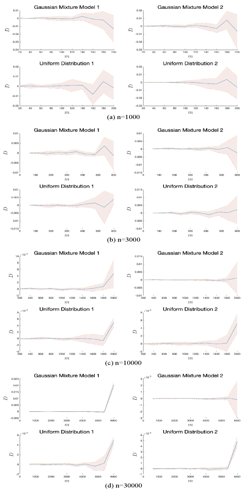
The experiments are conducted as follows. We generate 1000,3000,10000,30000 random samples from the four distributions separately, then use GKHR and GKH for sample selection under the low-budget setting, i.e., . The is set by . We report the results over ten independent runs in Figure 2, which shows that although the performance gap tends to grow as grows, when is relatively small, the performance of GKHR is similar to that of GKH. Therefore, under the low-budget setting, GKHR and GKH have similar performance on minimizing -MMD over various type of distributions, which convinces us that GKHR could work well in the sample selection task.
D.2 Datasets
For experiments, we choose five common datasets: CIFAR-10/100, SVHN, STL-10 and ImageNet. CIFAR-10 and CIFAR-100 contain 60,000 images with 10 and 100 categories, respectively, among which 50,000 images are for training, and 10,000 images are for testing; SVHN contains 73,257 images for training and 26,032 images for testing; STL-10 contains 5,000 images for training, 8,000 images for testing and 100,000 unlabeled images as extra training data. ImageNet spans 1,000 object classes and contains 1,281,167 training and 100,000 test images. The training sets of the above datasets are considered as the unlabeled dataset for sample selection.
D.3 Visualization of Selected Samples
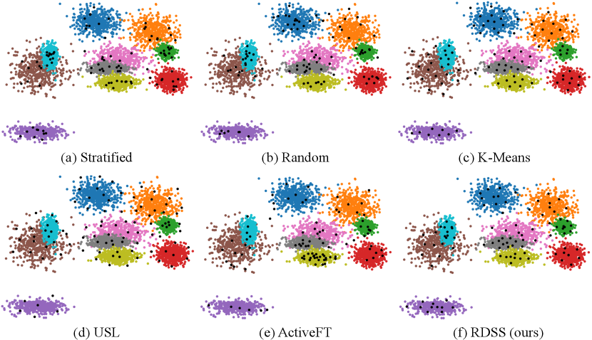
To offer a more intuitive comparison between various sampling methods, we visualized samples chosen by stratified, random, -Means, USL, ActiveFT and RDSS (ours). We generate 5000 samples from a Gaussian mixture model defined on with 10 components and uniform mixture weights. One hundred samples are selected from the entire dataset using different sampling methods. The visualisation results in Figure 3 indicate that our selected samples distribute more similarly with the entire dataset than other counterparts.
D.4 Computational Complexity and Running Time
We compute the time complexity of various sampling methods and recorded the time required to select 400 samples on the CIFAR-100 dataset for each method. The results are presented in Table 5, where represents the annotation budget, denotes the total number of samples, and indicates the number of iterations. The sampling time was obtained by averaging the duration of three independent runs of the sampling code on an idle server without any workload. As illustrated by the results, the sampling efficiency of our method surpasses that of all other methods except for random and stratified sampling. This discrepancy is likely because the execution time of other algorithms is affected by the number of iterations .
| Method | Time complexity | Time (s) |
|---|---|---|
| Random | ||
| Stratified | ||
| -means | ||
| USL | ||
| ActiveFT | ||
| RDSS (Ours) |
D.5 Implementation Details of Supervised Learning Experiments
We use ResNet-18 [16] as the classification model for all AL approaches and our method. Specifically, We train the models for epochs using SGD optimizer (initial learning rate=, weight decay=, momentum=) with batch size . Finally, we evaluate the performance with the Top-1 classification accuracy metric on the test set.
D.6 Direct Comparison with AL/SSAL
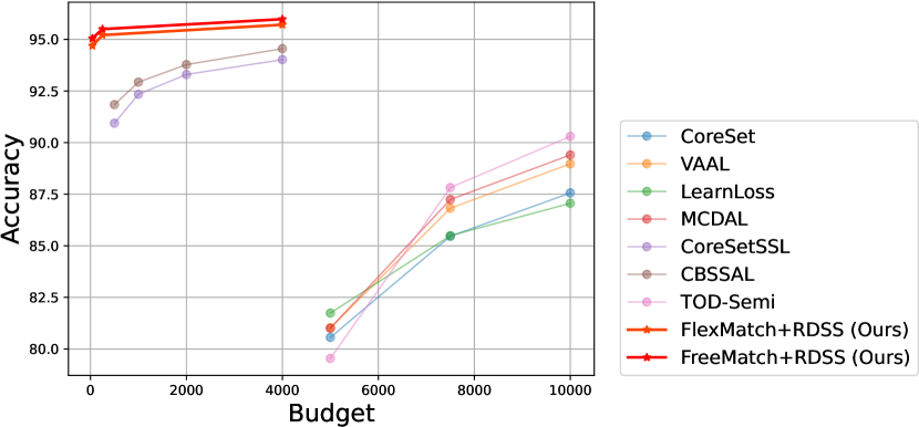
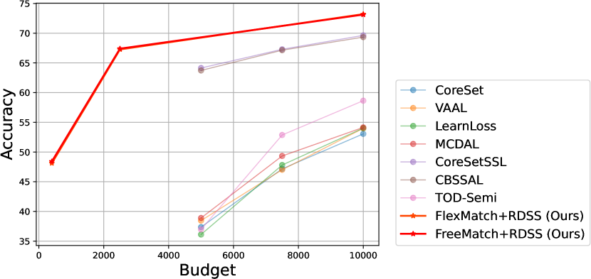
The comparative results with AL/SSAL approaches are shown in Figure 4 and Figure 5, respectively. The specific values corresponding to the comparative results in the above two figures are shown in Table 6. And the above results are from [8], [12] and [17].
| Dataset | CIFAR-10 | CIFAR-100 | ||||||||||||
| Budget | 40 | 250 | 500 | 1000 | 2000 | 4000 | 5000 | 7500 | 10000 | 400 | 2500 | 5000 | 7500 | 10000 |
| Active Learning (AL) | ||||||||||||||
| CoreSet [36] | - | - | - | - | - | - | 80.56 | 85.46 | 87.56 | - | - | 37.36 | 47.17 | 53.06 |
| VAAL [39] | - | - | - | - | - | - | 81.02 | 86.82 | 88.97 | - | - | 38.46 | 47.02 | 53.99 |
| LearnLoss [60] | - | - | - | - | - | - | 81.74 | 85.49 | 87.06 | - | - | 36.12 | 47.81 | 54.02 |
| MCDAL [8] | - | - | - | - | - | - | 81.01 | 87.24 | 89.40 | - | - | 38.90 | 49.34 | 54.14 |
| Semi-Supervised Active Learning (SSAL) | ||||||||||||||
| CoreSetSSL [36] | - | - | 90.94 | 92.34 | 93.30 | 94.02 | - | - | - | - | - | 63.14 | 66.29 | 68.63 |
| CBSSAL [12] | - | - | 91.84 | 92.93 | 93.78 | 94.55 | - | - | - | - | - | 63.73 | 67.14 | 69.34 |
| TOD-Semi [17] | - | - | - | - | - | - | 79.54 | 87.82 | 90.3 | - | - | 36.97 | 52.87 | 58.64 |
| Semi-Supervised Learning (SSL) with RDSS | ||||||||||||||
| FlexMatch+RDSS (Ours) | 94.69 | 95.21 | - | - | - | 95.71 | - | - | - | 48.12 | 67.27 | - | - | 73.21 |
| FreeMatch+RDSS (Ours) | 95.05 | 95.50 | - | - | - | 95.98 | - | - | - | 48.41 | 67.40 | - | - | 73.13 |
According to the results, we have several observations: (1) AL approaches often necessitate significantly larger labelling budgets, exceeding RDSS by 125 or more on CIFAR-10. This is primarily because AL paradigms are solely dependent on labelled samples not only for classification but also for feature learning. (2) SSAL and our methods leverage unlabeled samples, surpassing traditional AL approaches. However, this may not directly reflect the advantages of RDSS, as such performance enhancements could be inherently attributed to the SSL paradigm itself. Nonetheless, these experimental outcomes offer insightful implications: SSL may represent a more promising paradigm under scenarios with limited annotation budgets.
Appendix E Limitation
The choice of depends on the number of full unlabeled data points, independent of the information on the shape of data distribution. This may lead to a loss of effectiveness of RDSS on those datasets with complicated distribution structures. However, it outperforms fixed-ratio approaches on the datasets under different budget settings.
Appendix F Potential Societal Impact
Positive societal impact. Our method ensures the representativeness and diversity of the selected samples and significantly improves the performance of SSL methods, especially under low-budget settings. This reduces the cost and time of data annotation and is particularly beneficial for resource-constrained research and development environments, such as medical image analysis.
Negative societal impact. When selecting representative data for analysis and annotation, the processing of sensitive data may be involved, increasing the risk of data leakage, especially in sensitive fields such as medical care and finance. It is worth noting that most algorithms applied in these sensitive areas are subject to this risk.