Enhancing Trustworthiness of Graph Neural Networks with Rank-Based Conformal Training

Ting Wang¹, Zhixin Zhou², Rui Luo¹ Corresponding author:

Abstract

Graph Neural Networks (GNNs) has been widely used in a variety of fields because of their great potential in representing graph-structured data. However, lacking of rigorous uncertainty estimations limits their application in high-stakes. Conformal Prediction (CP) can produce statistically guaranteed uncertainty estimates by using the classifier’s probability estimates to obtain prediction sets, which contains the true class with a user-specified probability. In this paper, we propose a Rank-based CP during training framework to GNNs (RCP-GNN) for reliable uncertainty estimates to enhance the trustworthiness of GNNs in the node classification scenario. By exploiting rank information of the classifier’s outcome, prediction sets with desired coverage rate can be efficiently constructed. The strategy of CP during training with differentiable rank-based conformity loss function is further explored to adapt prediction sets according to network topology information. In this way, the composition of prediction sets can be guided by the goal of jointly reducing inefficiency and probability estimation errors. Extensive experiments on several real-world datasets show that our model achieves any pre-defined target marginal coverage while significantly reducing the inefficiency compared with state-of-the-art methods.

Code — https://github.com/CityU-T/RCP-GNN

Introduction

Graph Neural Networks (GNNs) has been widely used in many applications, such as weather forecasting (Lam et al. 2023), drug discovery (Li, Huang, and Zitnik 2022) and recommendation systems (Wu et al. 2022). However, predictions made by GNNs are inevitably present uncertainty. Though to understand the uncertainty in the predictions they produce can help to enhance the trustworthiness of GNNs (Huang et al. 2023), most existing uncertainty quantification (UQ) methods can not be easily adopted to graph-structured data (Stadler et al. 2021). Among various UQ methods, Conformal Prediction (CP) is an effective approach for achieving trustworthy GNNs (Wang et al. 2024). It relaxes the assumption of existing UQ methods, making it suitable for graph-structured data.

Instead of relying solely on uncalibrated predicted distribution $\mu(y|x)$ , CP constructs a prediction set that informs a plausible range of estimates aligned with the true outcome distribution $p(y|x)$ . The post-training calibration step make the output prediction sets provably include the true outcome with a user-specified coverage of $1-\alpha$ . A conformity score function is the key component for CP to quantify the agreement between the input and the candidate label.

Some studies have draw attention to the application of CP to graph-structured data (Clarkson 2023; H. Zargarbashi, Antonelli, and Bojchevski 2023; Lunde 2023; Lunde, Levina, and Zhu 2023; Marandon 2024). However, CP usually suffer inefficiency when there are no well-calibrated probabilities, with the intuition that larger prediction sets covers higher uncertainty. How to achieve desirable efficiency beyond validity is still a noteworthy challenge. Existing studies (Sadinle, Lei, and Wasserman 2019; Romano, Sesia, and Candes 2020) are typically changing the definition of the conformity scores for inefficiency reduction. The challenge is that CP is always used as a post-training calibration step, thus hindering its ability of underlying model to adapting to the prediction sets.

Recently, (Stutz et al. 2022; Bellotti 2021) try to using CP as a training step to make model parameter $\theta$ dependent with the calibration step, so as to modifying prediction sets towards reducing inefficiency. However, the integration of conformal training and GNNs still remain largely unexplored. The very resent work (Huang et al. 2023) proposed a conformal graph neural network which develops a topology-aware calibration step during training. Differently, we focus this problem with two lines. One is that a suitable conformity score is applied for GNNs who often struggle with miscalibration predictions (Wang et al. 2021). Another is that a conformal training framework based on the differentiable variant of this conformity score is designed to adjust the prediction sets along with model parameters’ optimization.

In conclusion, our contributions are two-fold. First, we propose a novel rank-based conformity scores that emphasizes the rank of prediction probabilities which is more robust to GNNs. Second, we develops a calibration step during training for adjusting the prediction sets along with the model parameters. We demonstrate that the rank-based conformal prediction method we introduce is performance-critical for efficiently constructing prediction sets with expected coverage rate. And the proposed method can outperform state-of-the-art methods for the graph node classification tasks on several popular network datasets in terms of the converge and inefficiency metrics.

Preliminaries

Let $G=(\mathcal{V},\mathcal{E},X)$ be a graph, where $\mathcal{V}$ is a set of nodes, $\mathcal{E}$ is a set of edges, and $X=\{x_{v}\}_{v\in\mathcal{V}}$ is the attributes. We denote $\mathcal{Y}$ as the discrete set of possible label classes. Let $\{(x_{v},y_{v})\}_{v\in D}$ be the random variables from the training data, where $x_{v}\in R^{d}$ is the $d$ -dimensional vector for node $v$ and $y_{v}\in\mathcal{Y}$ is its corresponding class. The training data $\mathcal{D}$ is randomly split into $\mathcal{D}_{tr}$ / $\mathcal{D}_{val}$ / $\mathcal{D}_{calib}$ as training/validation/calibration set. Note that the subset $\mathcal{D}_{calib}$ is withhold as calibration data for conformal prediction. Let $\{(x_{v})\}_{v\in D_{te}}$ be the random variables from the test data whose true labels $\{(y_{v})\}_{v\in D_{te}}$ is unknown for model. The goal of node classification tasks is to obtain a classifier $\mu:X\rightarrow Y$ , which can approximate the posterior distribution over classes $y_{v}\in Y$ . During the training step, $\{(x_{v},y_{v})\}_{v\in D_{tr}\cup D_{valid}}$ , $\{(x_{v})\}_{v\in D_{te}\cup D_{calib}}$ and the graph structure $(\mathcal{V},\mathcal{E})$ are available to GNN model for node representations.

Graph Neural Networks (GNNs)

In this paper, we focus on GNNs in the node classification scenario. GNNs is the most common encoder to learn compact node representations, which is generated by a series of propagation layers. For each layer $l$ , each node representation $h_{u}^{(l)}$ is updated by its previous representations $h_{u}^{(l-1)}$ , and aggregated features $\hat{m}_{u}^{(l)}$ obtained through passing message from its neighbours $\mathcal{N}_{(u)}$ :

h_{u}^{(l)}=\textrm{F}_{\textrm{upd}}(h_{u}^{(l-1)},\hat{m}_{u}^{(l)})\\

(1)

\hat{m}_{u}^{(l)}=\textrm{F}_{\textrm{agg}}(m_{(uv)},|v\in\mathcal{N}_{(u)})\\

(2)

m_{(uv)}=\textrm{F}_{\textrm{msg}}(h_{u}^{(l-1)},h_{v}^{(l-1)})

(3)

where $\textrm{F}_{\textrm{upd}}(\cdot)$ is a non-linear function to update node representations. $\textrm{F}_{\textrm{agg}}(\cdot)$ is the aggregation function while $\textrm{F}_{\textrm{msg}}(\cdot)$ is the message passing function. We use node representations in the last layer as the input of a classifier to obtain a prediction $\mu_{\theta}(x)$ .

For CP on GNNs, a valid coverage guarantee requires the exchangeability of the calibration and test data. Since our model is transduction node classification, the calibration examples are drawn exchangeability from the test distribution following (Huang et al. 2023).

Conformal Prediction

For a new test point $x_{n+1}$ , the goal of CP is to construct a reasonably small prediction set $C(x_{n+1})$ , which contains corresponding true label $y_{n+1}\in\mathcal{Y}$ with pre-defined coverage rate $1-\alpha$ :

P(y_{n+1}\in C(x_{n+1}))\geq 1-\alpha

(4)

where $\alpha\in[0,1]$ is the user-specific miscoverage rate. The standard CP is usually conduct at test time after the classification model $\mu_{\theta}$ is trained, which is achieved in two steps: 1) In the calibration step, a cut-off threshold $\hat{\eta}$ is calculated by the quantile function of the conformity scores $V:X\times Y\rightarrow R$ on the hold-out calibration set $\mathcal{D}_{calib}$ . During calibration, the true classes $y_{i}$ are used for computing the threshold to ensure coverage $1-\alpha$ . 2) In the prediction step, the prediction sets $C(x)$ depending on the threshold $\hat{\eta}$ and the model parameters $\theta$ are constructed. The conformity score function is designed to measure the predicted probability of a class, and it is typically changed for various objectives. Two popular conformity scores are described in details below.

Threshold Prediction Set (THR)

The threshold $\hat{\eta}$ for THR (Sadinle, Lei, and Wasserman 2019) is calculated by the $\alpha$ quantile of the conformity scores:

\hat{\eta}=Q(\{V(x_{i},y_{j})|i\in\mathcal{D}_{calib}\},\alpha(1+\frac{1}{|\mathcal{D}_{calib}|}))

(5)

where $Q(\cdot)$ is the quantile function. The prediction sets including labels with sufficiently large prediction values are constructed by thresholding probabilities:

C(x)=\{k\in\mathcal{Y}:V(x,k)\geq\hat{\eta}\}

(6)

V(x,k)=\mu_{k}(x)

(7)

Adaptive Prediction Set (APS)

APS (Romano, Sesia, and Candes 2020) takes the cumulative sum of ordered probabilities $\mu_{\pi(1)}(x)>\mu_{\pi(2)}(x)>\cdots\mu_{\pi(|\mathcal{Y}|)}(x)$ for prediction set construction:

C(x)=\{k\in\mathcal{Y}:V(x,k)\leq\hat{\eta}\}

(8)

V(x,k)=\sum_{j=1}^{k}\mu_{\pi(j)}(x)

(9)

where $\pi$ is a permutation of $\mathcal{Y}$ , and the $(1-\alpha)(1+1/|\mathcal{D}_{calib}|)$ -quantile is also required for calibration to ensure marginal coverage.

RANK: Rank-based Conformal Prediction

Following our previous work (Luo and Zhou 2024), we advancing CP to GNNs through rank-based conformity scores, named RANK, to directly reduce the inefficiency. Assuming that a higher value of $\mu_{k}(x_{i})$ indicates a greater likelihood of $x_{i}$ belonging to class $k$ . Consequently, if class $k$ is included in the prediction set, and $\mu_{k^{\prime}}(x_{i})>\mu_{k}(x_{i})$ satisfied, then $k^{\prime}$ must be in the prediction set. According to this assumption, the size of the prediction set including the true label can be evaluated in the calibration step. The smallest prediction set that includes the true label $y_{i}$ will be constructed by the rank of $\mu_{y_{i}}(x_{i})$ within the sequence $\{\mu_{1}(x),\cdots\mu_{\mathcal{Y}}(x)\}$ .

Ranked Threshold Prediction Sets

For each $i\in\mathcal{D}_{calib}$ , the following rank is defined to establish a rule to choose labels:

r_{i}=\mathrm{rank}\;\mathrm{of}\;\mu_{y_{i}}(x_{i})\;\mathrm{in}\;\{\mu_{k}(x_{i}):k\in\mathcal{Y}\}

(10)

so that the order statistics can be find: $r_{(1)}\geq r_{(2)}\cdots\geq r_{(n)}$ . Let $r_{\alpha}^{*}=r_{(\lfloor(n+1)\alpha\rfloor)}$ , either top- $(r_{\alpha}^{*}-1)$ or top- $(r_{\alpha}^{*})$ classes will be included in the prediction set. The top- $(r_{\alpha}^{*})$ classes refers to the classes corresponding to the $(r_{\alpha}^{*})$ -th largest prediction values. To achieve the target coverage, the $\mu^{*}$ is defined to determine when the $(r_{\alpha}^{*})$ -th class should be included in the prediction sets:

\mu^{*}=\lceil np\rceil\textrm{-th largest value in }\{\hat{\mu}_{r_{\alpha}^{*}}(x_{i}):i\in\mathcal{D}_{calib}\}

(11)

where $n$ is the size of $\mathcal{D}_{calib}$ , $p$ is the proportion of instances we should included in the $r_{a}^{*}$ -th label, and $\hat{\mu}_{k}(x_{i})$ denotes the $k$ -th order statistics in $(\mu_{1}(x_{i}),...,\mu_{n}(x_{i}))$ . The prediction set is defined as follows:

C(x)=\left\{\begin{array}[]{ll}&\{k\in\mathcal{Y}:\hat{\mu}_{k}(x)\geq\hat{\mu}_{r_{\alpha}^{*}}(x)\},\\ &\textrm{if}\quad\hat{\mu}_{r_{\alpha}^{*}}(x)\geq\mu^{*};\\ &\{k\in\mathcal{Y}:\hat{\mu}_{k}(x)\geq\hat{\mu}_{r_{{\alpha}^{*}-1}}(x)\},\\ &\textrm{otherwise};\\ \end{array}\right.

(12)

According to above analysis, the rank-based conformity scores calculated on the calibration set can be defined following:

\begin{split}&V(x_{i},y_{i})=\\ &[\mathrm{rank}\;\mathrm{of}\;\hat{\mu}_{y_{i}}(x_{i})\;\mathrm{in}\;\{\hat{\mu}_{1}(x_{i}),\cdots,\hat{\mu}_{\mathcal{Y}}(x_{i})\}]-1\\ &+\frac{1}{n}[\mathrm{rank}\;\mathrm{of}\;\hat{\mu}_{y_{i}}(x_{i})\;\mathrm{in}\;\{\hat{\mu}_{y_{i}}(x_{1}),\cdots,\hat{\mu}_{y_{i}}(x_{n})\}]\end{split}

(13)

and the quantile $Q$ as the $\lfloor(n+1)\alpha\rfloor$ -th largest value among the conformity scores, defining the prediction set is equivalent to selecting the calibration samples that satisfy the condition $V(x_{i},y_{i})\leq Q$ , is employed to construct the prediction set with $1-\alpha$ coverage.

RCP-GNN: Rank-Based Conformal Prediction on Graph Neural Networks

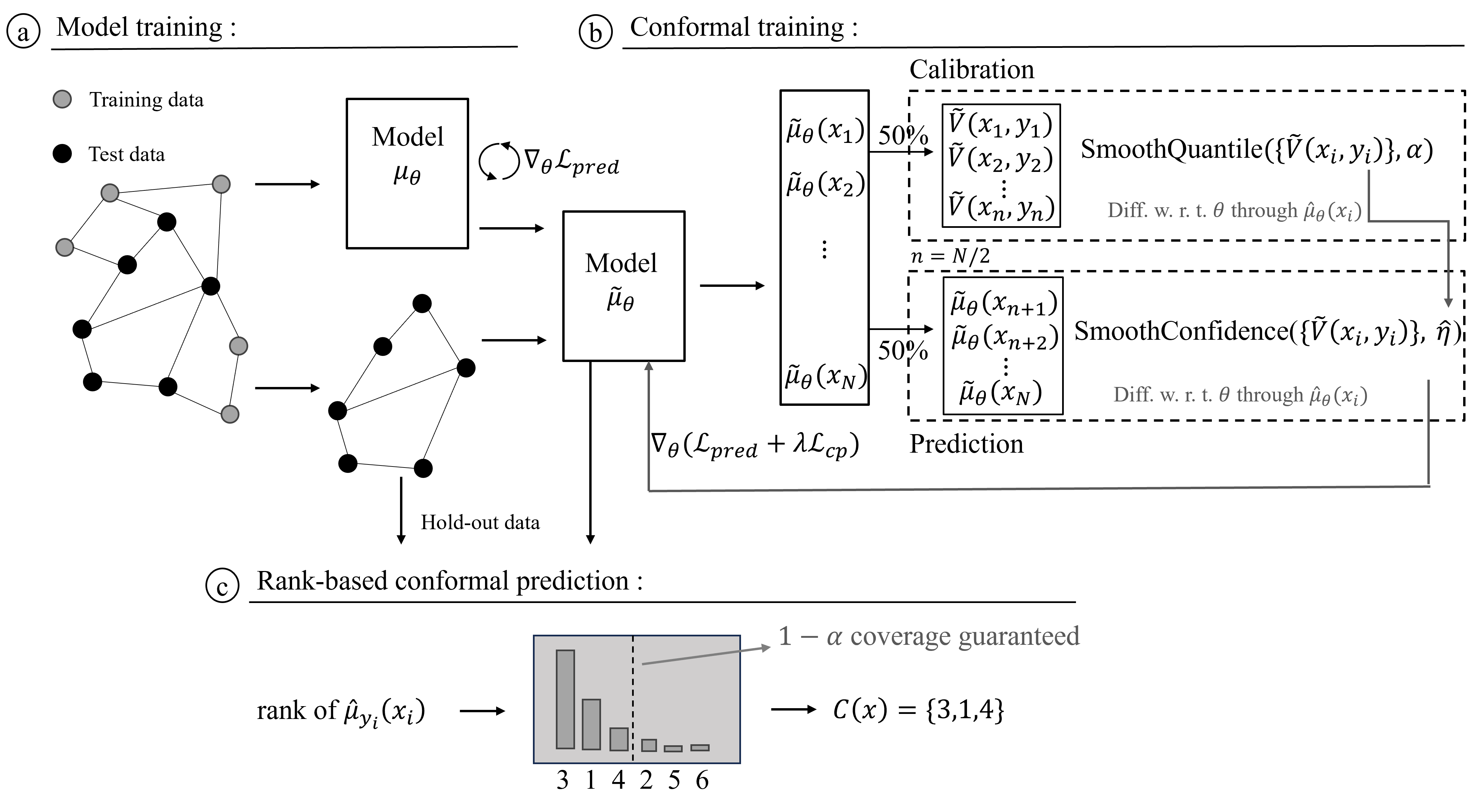
Refer to caption — Figure 1: The framework of RCP-GNN. (a) Model training stage. The GNN model $\textrm{GNN}_{base}$ is trained by optimizing a prediction loss using a standard deep learning step. And the prediction probabilities of node $i$ : $\mu(x_{i})$ is obtained. (b) Conformal training stage. The novel rank-based conformal training step is proposed to adjust the prediction set for desirable properties jointly with improve estimation accuracy. The topology-aware correction model $\textrm{GNN}_{cor}$ that takes $\tilde{\mu}(x)$ as the output is updated by the conformal training step. (c) Rank-based Conformal Prediction. The rank-based CP is employed to produce a prediction set based on $\tilde{\mu}$ which includes true label with a user-specified probability.

We propose RCP-GNN into two-stage: model training stage and conformal training stage, as Figure 1 shows. In model training stage, the base model $\textrm{GNN}_{base}$ is trained only by prediction loss (i.e., cross-entropy loss), and $\mu(X)$ is the estimator of base model.

In conformal training stage, the correct model $\textrm{GNN}_{cor}$ is trained by both prediction loss and conformity loss. We set $\tilde{\mu}(X)=\mathrm{GNN}_{cor}(\mu(X),G)$ as the estimator of correct model. The prediction set will be optimized when CP performing on each mini-batch. For the reason that training with original rank-based CP may cause limited gradient flow, a differentiable implementation for RANK is designed to enable smooth sorting and ranking, and is further used to construct the conformity loss function, which sharpens the prediction set.

Conformal Training

We try to train our model end-to-end with the conformal wrapper in order to allow fine-grained control over the prediction sets $C(x)$ . Following the split CP approach (Lei, Rinaldo, and Wasserman 2013), we randomly split the test data set $\mathcal{D}_{te}$ into folds with 50%/50% as $\hat{\mathcal{D}}_{calib}$ / $\hat{\mathcal{D}}_{te}$ for calibration and constructing prediction sets. Before splitting the test data, a fraction of test data is withhold for further standard rank-based conformal prediction stage.

Differentiable Prediction and Calibration Steps

A differentiable CP method which involves differentiable prediction and calibration step is defined for the training process: 1) In the prediction step, the prediction sets $C(x)$ w.r.t. the threshold $\hat{\eta}$ and the predictions $\tilde{\mu}_{\theta}(x)$ is set to be differentiable. 2) In the calibration step, the conformity scores w.r.t. the predictions $\tilde{\mu}_{\theta}(x)$ as well as quantile function is set to be differentiable. Notably, the predictions $\tilde{\mu}_{\theta}(x)$ are always differentiable throughout calibration and prediction steps. Therefore, The key component of differentiating through CP is the differentiable conformity scores and the differentiable quantile computation.

Given the prediction probabilities $\tilde{\mu}(X)$ , the smooth sorting designed by a $\mathrm{sigmoid}(x)=\frac{1}{1+e^{-x}}$ function and a temperature hyper-parameter $\tau\in[0,1]$ is utilized to replace “hard” rank manipulation for the smoothed rank-based conformity scores:

\tilde{V}(x_{i},k)=\sum_{j=1}^{|\mathcal{Y}|}\textrm{sigmoid}(\frac{\tilde{\mu}_{j}(x_{i})-\tilde{\mu}_{k}(x_{i})}{\tau})

(14)

After that, a differentiable quantile computation is employed for smoothed thresholding under smooth sorting.

\hat{\eta}=\tilde{Q}(\{V(x_{i},y_{i})|i\in\hat{\mathcal{D}}_{calib}\},\alpha(1+\frac{1}{|\hat{\mathcal{D}}_{calib}|}))

(15)

where $\tilde{Q}(\cdot)$ is the smooth quantile function that are well-established in (Blondel et al. 2020; Chernozhukov, Fernández-Val, and Galichon 2007).

Loss Function

The conformal training stage performs differentiable CP on data batch during stochastic gradient descent (SGD) training. As mentioned above, the $\hat{\eta}$ is calibrated by $\alpha(1+1/{\hat{|\mathcal{D}}_{calib}|})$ -quantile of the conformity scores in a differentiable way. Under the constraint of hyper-parameter $\tau$ , we empirically make coverage close to $1-\alpha$ by approximating “hard” sorting. Then we propose a conformity loss function to further optimize the inefficiency through training. Given the estimator $\tilde{\mu}_{j}(x_{i})$ for the conditional probability of $Y$ being class $k\in\mathcal{Y}$ at $X=x_{i}$ and the true label $y_{i}$ . Similar with Eq.14, the smooth conformity scores on test data is defined as:

\tilde{V}(x_{i},y_{i})=\sum_{k=1}^{|\mathcal{Y}|}\textrm{sigmoid}(\frac{\tilde{\mu}_{k}(x_{i})-\tilde{\mu}_{y_{i}}(x_{i})}{\tau})

(16)

Given $i\in\hat{\mathcal{D}}_{calib}$ , a soft assignment (Stutz et al. 2022; Huang et al. 2023) of each class $k$ to the prediction set is defined smoothly as follows:

c_{i}=\textrm{max}(0,\sum_{k\in\mathcal{Y}}{\textrm{sigmoid}(\frac{\tilde{V}(x_{i},k)-\hat{\eta}}{\tau})}-\kappa)

(17)

Then the conformity loss function is defined by:

\mathcal{L}_{cp}=\frac{1}{|\hat{\mathcal{D}}_{te}|}\frac{1}{|\mathcal{Y}|}\sum\nolimits_{i\in\hat{\mathcal{D}}_{te}}{c_{i}}

(18)

Thus, the loss function optimized in conformal training stage is defined as follows:

\mathcal{L}=\mathcal{L}_{pred}+\lambda*\mathcal{L}_{cp}

(19)

where $\lambda$ is a hyper-parameter to balance the items and $\mathcal{L}_{pred}$ is the prediction loss for optimizing model parameters $\theta$ :

\begin{split}&\mathcal{L}_{pred}=\\ &\!-\!\sum_{i\in\mathcal{D}_{tr}}[y_{i}log(\tilde{\mu}_{\theta}(x_{i}))\!+\!(1\!-\!y_{i})log(1\!-\!\tilde{\mu}_{\theta}(x_{i}))]\end{split}

(20)

After training, standard rank-based CP are conduct on $\tilde{\mu}(X)$ for prediction sets construction.

Experiment

We conduct experiments to demonstrate the advantages of our model over existing methods in achieving empirical marginal coverage for graph data, as well as the efficiency improvement. We also conduct systematic ablation and parameter analysis to show the robustness of our model.

Experiment Setup

Dataset

We choose eight popular graph-structured datasets, i.e., Cora, DBLP, CiteSeer and PubMed (Yang, Cohen, and Salakhudinov 2016), Amazon-Computers and Amazon-Photo, Coauthor-CS and Coauthor-Physics (Shchur et al. 2019) for evaluation. We randomly split them with 20%/10%/70% as training/validation/testing set following previous works (Huang et al. 2023; Stutz et al. 2022). The statistical information of datasets is summarized in Table 1.

Data	# Nodes	# Edges	# Features	# Labels
Cora	2,995	16,346	2,879	7
DBLP	17,716	105,734	1,639	4
CiteSeer	4,230	10,674	602	6
PubMed	19,717	88,648	500	3
Computers	13,752	491,722	767	10
Photos	7,650	238,162	745	8
CS	18,333	163,788	6,805	15
Physics	34,493	495,924	8,415	5

Table 1: Statistics of Datasets.

Baseline

We consider both general statistical calibration approaches temperate, i.e., temperate scaling (Guo et al. 2017), vector scaling (Guo et al. 2017), ensemble temperate scaling (Zhang, Kailkhura, and Han 2020) and SOTA GNN-specific calibration methods, i.e., CaGCN (Wang et al. 2021), GATS (Hsu et al. 2022) and CF-GNN(Huang et al. 2023).

Implementation.

Our model and baselines are trained on Intel(R) Core(TM) i7-5820K CPU @ 3.30GHz, 64G RAM computing server, equipped with NVIDIA GTX TITAN X graphics cards. All hyper-parameters are chosen via random search. Details of hyper-parameter setting ranges are listed in Table 2.

Param.	Value
$\lambda$	{1e-2, 1e-1, 1, 10}
$\tau$	{1e-2, 1e-1, 1, 10}
$\kappa$	{0, 1}
GNN Layers	{1, 2, 3, 4}
GNN Hidden Dimension	{16, 32, 64, 128, 256}
Learning Rate	{1e-1, 1e-2, 1e-3, 1e-4}

Table 2: Hyper-parameters setting.

Metrics

Marginal coverage and inefficiency are two commonly used metrics for measuring the performance of CP. Given the test set $\mathcal{D}_{te}$ , the marginal coverage metric is defined as follows:

\textrm{Coverage}:=\frac{1}{|\mathcal{D}_{te}|}\sum_{i\in\mathcal{D}_{te}}{\delta[y_{i}\in C(x_{i})]}

(21)

where $\delta[\cdot]$ is the indicator function, it is 1 when its argument is true and 0 otherwise. The coverage is empirically guaranteed when marginal coverage exceeds $1-\alpha$ . In cases where it exceeds this threshold, the results improve as they get closer to the target. The marginal coverage guarantee ensures that the output prediction sets for new test points provably include the true outcome with probability at least $1-\alpha$ . Then we focus on desirable prediction set size to enable further comparisons across CP methods. The inefficiency metric is defined by the size of the prediction set:

\textrm{Ineff}:=\frac{1}{|\mathcal{D}_{te}|}\sum_{i\in\mathcal{D}_{te}}{|C(x_{i})|}

(22)

where smaller values indicate better performance.

Results

Marginal Coverage Results.

Datasets	Temp. Scale.	Vector Scale.	Ensemble TS	CaGCN	GATS	CF-GNN	RCP-GNN
Cora	0.946(.003)	0.944(.004)	0.947(.003)	0.939(.005)	0.939(.005)	0.952(.001)	0.950(.002)
DBLP	0.920(.009)	0.921(.009)	0.920(.008)	0.922(.004)	0.921(.004)	0.952(.001)	0.950(.001)
CiteSeer	0.952(.004)	0.951(.004)	0.953(.003)	0.949(.005)	0.951(.005)	0.953(.001)	0.951(.001)
PubMed	0.899(.002)	0.899(.003)	0.899(.002)	0.898(.003)	0.898(.002)	0.953(.001)	0.950(.002)
Computers	0.929(.002)	0.932(.002)	0.930(.002)	0.926(.003)	0.925(.002)	0.952(.001)	0.951(.001)
Photo	0.962(.002)	0.963(.002)	0.964(.002)	0.956(.002)	0.957(.002)	0.953(.001)	0.951(.001)
CS	0.957(.001)	0.958(.001)	0.958(.001)	0.954(.003)	0.957(.001)	0.952(.001)	0.950(.001)
Physics	0.969(.000)	0.969(.000)	0.969(.000)	0.968(.001)	0.968(.000)	0.952(.001)	0.950(.001)

Table 3: Empirical marginal coverage of different methods with

\alpha=0.05

. The result takes the average and standard deviation across 10 runs with 100 calib/test splits. Marked: Covered, Closest.

Methods	Cora	DBLP	CiteSeer	Computers	Photo
Temp. Scale.	1.37	1.19	1.14	1.31	1.15
Vector Scale.	1.36	1.20	1.15	1.25	1.13
Ensemble TS.	1.37	1.19	1.14	1.30	1.15
CaGCN.	1.41	1.18	1.19	1.22	1.14
GATS	1.33	1.18	1.16	1.28	1.12
CF-GNN	1.72	1.23	0.99	1.81	1.66
RCP-GNN	1.18(11.28% $\downarrow$ )	1.17(0.85% $\downarrow$ )	0.97(2.02% $\downarrow$ )	1.20(1.64% $\downarrow$ )	1.04(7.14% $\downarrow$ )

Table 4: Empirical inefficiency results of different methods across various datasets at test time with

\alpha=0.1

. Marked: First. Second. The average inefficiency reduction relative to the best results of baselines in percentage is reported in parentheses.

Methods	Cora		CiteSeer		Photo
Methods	Coverage	Size	Coverage	Size	Coverage	Size
RCP-THR	0.954	1.65	0.953	1.57	0.953	1.26
RCP-APS	0.952	2.32	0.952	1.86	0.953	1.87
w/o Conf.Tr.	0.950	2.08	0.951	1.97	0.951	2.00
RCP-GNN	0.950	1.92	0.951	1.26	0.951	1.23

Table 5: Empirical marginal coverage and inefficiency of variants at

\alpha=0.05

. Marked: Best.

The marginal coverage of different methods are reported in Table 3. All methods use the same pre-trained base model to avoid randomness. The results that achieves the target coverage are marked with underline. The most closest values among covered coverage are marked by bold font. Some observations are introduced as follows:

Temperate scaling, vector scaling and ensemble temperate scaling do not perform well because they lack to aware the topology information in graphs. Although CaGCN and GATS try to integrate topology information to per-node temperature scaling, their performance is still unsatisfactory because they only use CP as a post-training calibration step. Among SOTA methods, only CF-GNN reached target coverage on all datasets. It confirms that fixing prediction sets during training is helpful for reliable uncertainty estimates.

Among all methods, our model successfully reached target coverage on all datasets. Moreover, our model empirically achieves coverage rate closest to target. In summary, our model achieves superior empirical marginal coverage than existing methods.

Inefficiency Results.

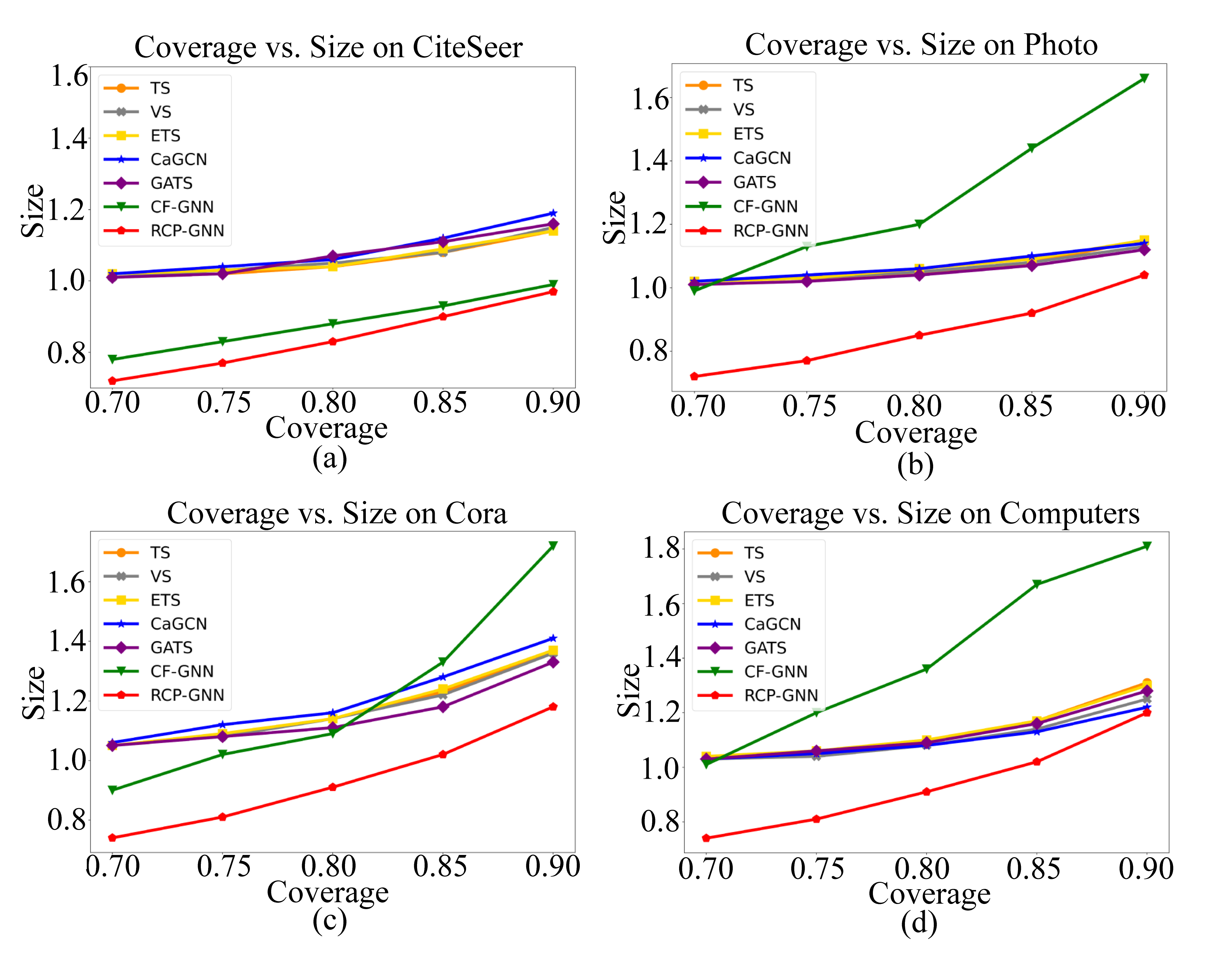
In Table 4, we summarize the inefficiency reductions of our methods in comparison to other baselines. It can be observed that our model achieve efficiency improvement across datasets with up to 11.28% reduction in the prediction size. We also empirical present the inefficiency of different methods on various tasks for $\alpha$ ranging from 0.1 to 0.3 in Figure 2. Though CF-GNN try to reduce inefficiency through training with conformal prediction, it does not consistently improve inefficiency across all datasets. Specifically, on Amazon-Photo and Amazon-Computers, efficiency becomes even worse. Our RCP-GNN, in contrast, reduces inefficiency consistently.

The reason may be that RCP-GNN constructs and adjusts prediction sets based on ranking and probability of the labels, while CF-GNN only rely on assumptions about the model’s probabilities. Therefore, CF-GNN may not fully capture the model’s uncertainty, which hinders its performance. Additionally, RCP-GNN uses differentiable method to approximate “hard” sorting procedure, which helps to improve the performance and scalability of our framework.

In summary, our model can significantly reduce the inefficiency while maintaining satisfactory marginal coverage compared with other state-of-the-art methods.

Ablation Study

We conduct ablations in Table 5 to test main components in RCP-GNN. 1) RCP-THR. It is a variant of RCP-GNN that using THR to compute the conformity scores. Since the THR conformity scores is naturally differentiable w.r.t. the model parameters $\theta$ according to Eq. 7, we only need to ensure the quantile function differentiable in the conformal training stage. 2) RCP-APS. Similar to RCP-THR, this variant leverage APS to compute the conformity scores. The differentiable implementation closely follows the one for RANK outlined in Eq. 14:

V(x_{i},y_{i})=\sum_{k=1}^{|\mathcal{Y}|}\textrm{sigmoid}(\frac{\tilde{\mu}_{y_{i}}(x_{i})-\tilde{\mu}_{k}(x_{i})}{\tau})\tilde{\mu}_{k}(x_{i})

(23)

3) w/o Conf.Tr. In order to figure out the power of conformal training step, we remove the conformity loss and replace it with standard prediction loss. Compared with RCP-THR and RCP-APS, our model can achieve pre-defined marginal coverage with satisfactory inefficiency reduction, which demonstrates that the rank-based conformal prediction component is performance-critical to ensure valid coverage guarantees while simultaneously enhancing efficiency. Compared with w/o Conf.Tr., our model achieves consistent efficiency improvement, which demonstrates that prediction sets can be optimized along with conformal training.

Hyper-Parameter Sensitivity

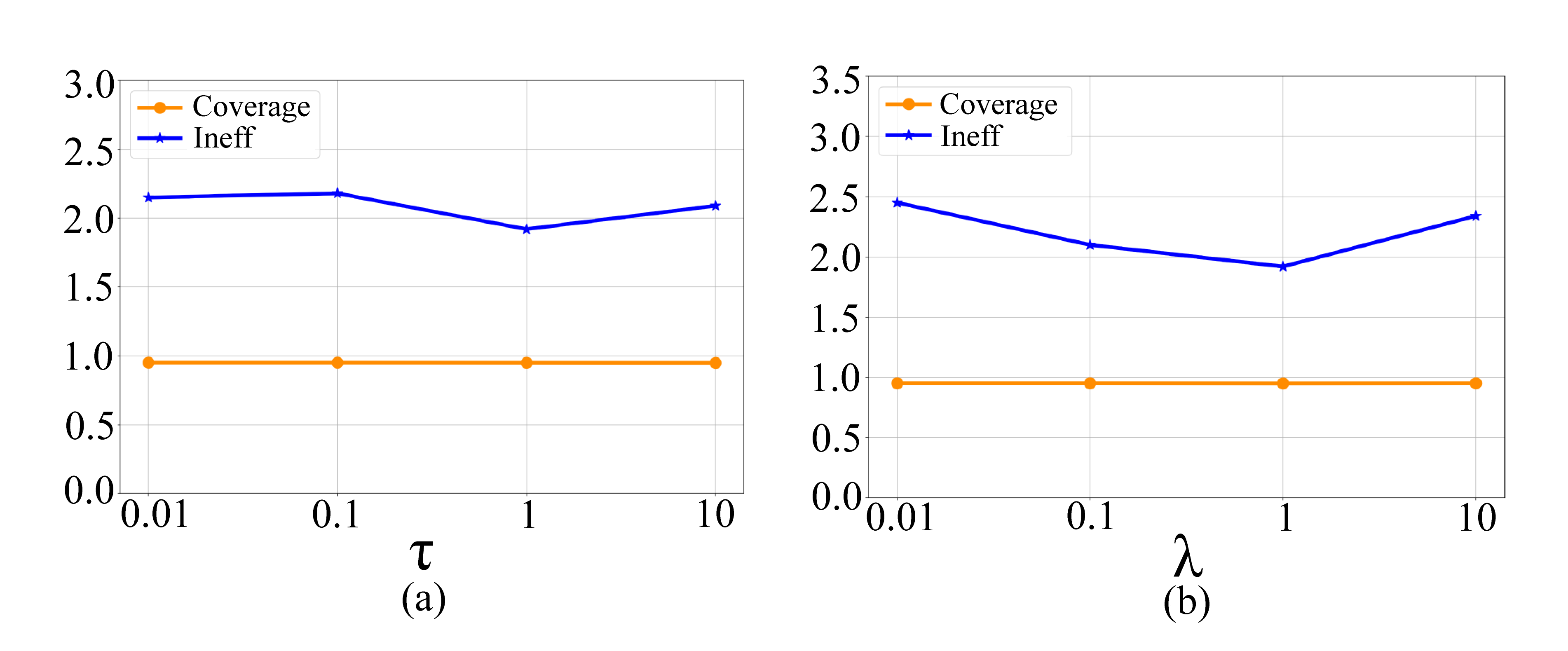
We also conduct experiments for major hyper-parameters of our model to test the robustness of RCP-GNN. In concrete, the hyper-parameter temperature is changed from 0.01 to 10 and the results show that our model is not sensitivity to the temperature. And we select the median value 1 for its relatively better performance. The hyper-parameter $\lambda$ in Eq. 19 is used to balance the prediction loss and the conformity loss. We report the converge and inefficiency results as $\lambda$ changes from 0.01 to 10 and we can observe that a proper weight of conformity loss can help to inefficiency reduction.

Related Works

Uncertainty Quantification in Deep Learning.

It is important for trustworthy modern deep learning models to mitigate overconfidence (Wang et al. 2020; Slossberg et al. 2022; Jiang et al. 2018). Uncertainty quantification (UQ), which aims to construct model-agnostic uncertain estimates, have great potential in many high-stakes applications (Abdar et al. 2021; Gupta et al. 2021; Guo et al. 2017; Kull et al. 2019; Zhang, Kailkhura, and Han 2020). Most of existing UQ methods rely on the i.i.d assumption. Thus make them be not easily adopt to inter-dependency graph-structure data. Some network principle-based UQ methods (Wang et al. 2021; Hsu et al. 2022) designing for GNNs have been proposed in recent years. However, these UQ methods fail to achieve valid coverage guarantee.

Standard Conformal Prediction.

Conformal prediction (CP) is early proposed on (Vovk, Gammerman, and Shafer 2005). Compared with other CP framework, e.g., cross-validation (Vovk 2015) or jackknife (Barber et al. 2021), most approaches follow a split CP method (Lei, Rinaldo, and Wasserman 2013), where a held-out calibration set is necessary. For the reason that it defines faster and more scalable CP algorithms. However, it sacrifices statistical efficiency.

Different variants of CP are struggled to the balance between statistical and computational efficiency. Some contributions made in conformity score function have been explored (Sadinle, Lei, and Wasserman 2019; Angelopoulos et al. 2021; Romano, Sesia, and Candes 2020) for inefficiency reduction. Other studies (Bates et al. 2021; Yang and Kuchibhotla 2024) have explored in the context of ensembles to obtain smaller confidence sets while avoiding to sacrifice the obtained empirical coverage. But these methods do not solve the major limitation of CP methods: the model is independent, leaving CP little to no control over the prediction sets (Guzmán-rivera, Batra, and Kohli 2012). Recently, the work of (Bellotti 2021) and (Stutz et al. 2022) try to better integrated CP into deep learning models by simulating CP during training to make full use of CP benefits. For GNNs, how to define a trainable calibration step still remains an open space for exploration.

Conformal Prediction for Graphs.

Some efforts have been done for CP to GNNs. The work of (Wijegunawardana, Gera, and Soundarajan 2020) adapted CP for node classification to achieve bounded error, and (Clarkson 2023) adapted weighted exchangeability without any lowerbound on the coverage. Furthermore, the assumption for a valid guarantee that the exchangeability between the calibration set and the test set is proved by (H. Zargarbashi, Antonelli, and Bojchevski 2023; Huang et al. 2023), which makes CP applicable to transduction node classification tasks. Different from these works, we leverage the rank of prediction probabilities of nodes to reduce its miscalibration. We also provide its differentiable variant for calibration during training to make prediction sets become aware of network topology information.

Conclusion

In this work, we extend CP to GNNs by proposing a trainable rank-based CP framework for marginal coverage guaranteed and inefficiency reduction. In future work we will focus on more tasks like link prediction, and extensions to graph-based applications such as molecular prediction and recommendation systems.

Acknowledgements

The work described in this paper was partially supported by grants from City University of Hong Kong (Project No. 9610639, 6000864).

References

Abdar et al. (2021) Abdar, M.; Pourpanah, F.; Hussain, S.; Rezazadegan, D.; Liu, L.; Ghavamzadeh, M.; Fieguth, P.; Cao, X.; Khosravi, A.; Acharya, U. R.; Makarenkov, V.; and Nahavandi, S. 2021. A review of uncertainty quantification in deep learning: Techniques, applications and challenges. Information Fusion, 76: 243–297.
Angelopoulos et al. (2021) Angelopoulos, A. N.; Bates, S.; Jordan, M.; and Malik, J. 2021. Uncertainty Sets for Image Classifiers using Conformal Prediction. In International Conference on Learning Representations.
Barber et al. (2021) Barber, R. F.; Candes, E. J.; Ramdas, A.; and Tibshirani, R. J. 2021. Predictive inference with the jackknife+. The Annals of Statistics, 49(1): 486–507.
Bates et al. (2021) Bates, S.; Angelopoulos, A.; Lei, L.; Malik, J.; and Jordan, M. 2021. Distribution-free, risk-controlling prediction sets. Journal of the ACM (JACM), 68(6): 1–34.
Bellotti (2021) Bellotti, A. 2021. Optimized conformal classification using gradient descent approximation. arXiv:2105.11255.
Blondel et al. (2020) Blondel, M.; Teboul, O.; Berthet, Q.; and Djolonga, J. 2020. Fast Differentiable Sorting and Ranking. In Proceedings of the 37th International Conference on Machine Learning, volume 119, 950–959. PMLR.
Chernozhukov, Fernández-Val, and Galichon (2007) Chernozhukov, V.; Fernández-Val, I.; and Galichon, A. 2007. Quantile and probability curves without crossing. Econometrica, 78: 1093–1125.
Clarkson (2023) Clarkson, J. 2023. Distribution Free Prediction Sets for Node Classification. In Proceedings of the 40th International Conference on Machine Learning, volume 202, 6268–6278. PMLR.
Guo et al. (2017) Guo, C.; Pleiss, G.; Sun, Y.; and Weinberger, K. Q. 2017. On Calibration of Modern Neural Networks. In Proceedings of the 34th International Conference on Machine Learning, volume 70, 1321–1330. PMLR.
Gupta et al. (2021) Gupta, K.; Rahimi, A.; Ajanthan, T.; Mensink, T.; Sminchisescu, C.; and Hartley, R. 2021. Calibration of Neural Networks using Splines. In International Conference on Learning Representations.
Guzmán-rivera, Batra, and Kohli (2012) Guzmán-rivera, A.; Batra, D.; and Kohli, P. 2012. Multiple Choice Learning: Learning to Produce Multiple Structured Outputs. In Advances in Neural Information Processing Systems, volume 25. Curran Associates, Inc.
H. Zargarbashi, Antonelli, and Bojchevski (2023) H. Zargarbashi, S.; Antonelli, S.; and Bojchevski, A. 2023. Conformal Prediction Sets for Graph Neural Networks. In Proceedings of the 40th International Conference on Machine Learning, volume 202, 12292–12318. PMLR.
Hsu et al. (2022) Hsu, H. H.-H.; Shen, Y.; Tomani, C.; and Cremers, D. 2022. What Makes Graph Neural Networks Miscalibrated? In Advances in Neural Information Processing Systems, volume 35, 13775–13786. Curran Associates, Inc.
Huang et al. (2023) Huang, K.; Jin, Y.; Candes, E.; and Leskovec, J. 2023. Uncertainty Quantification over Graph with Conformalized Graph Neural Networks. In Advances in Neural Information Processing Systems, volume 36, 26699–26721. Curran Associates, Inc.
Jiang et al. (2018) Jiang, H.; Kim, B.; Guan, M. Y.; and Gupta, M. 2018. To trust or not to trust a classifier. In Proceedings of the 32nd International Conference on Neural Information Processing Systems, NIPS’18, 5546–5557. Red Hook, NY, USA: Curran Associates Inc.
Kull et al. (2019) Kull, M.; Perello Nieto, M.; Kängsepp, M.; Silva Filho, T.; Song, H.; and Flach, P. 2019. Beyond temperature scaling: Obtaining well-calibrated multi-class probabilities with Dirichlet calibration. In Advances in Neural Information Processing Systems, volume 32. Curran Associates, Inc.
Lam et al. (2023) Lam, R.; Sanchez-Gonzalez, A.; Willson, M.; Wirnsberger, P.; Fortunato, M.; Alet, F.; Ravuri, S.; Ewalds, T.; Eaton-Rosen, Z.; Hu, W.; Merose, A.; Hoyer, S.; Holland, G.; Vinyals, O.; Stott, J.; Pritzel, A.; Mohamed, S.; and Battaglia, P. 2023. Learning skillful medium-range global weather forecasting. Science, 382(6677): 1416–1421.
Lei, Rinaldo, and Wasserman (2013) Lei, J.; Rinaldo, A.; and Wasserman, L. A. 2013. A conformal prediction approach to explore functional data. Annals of Mathematics and Artificial Intelligence, 74: 29 – 43.
Li, Huang, and Zitnik (2022) Li, M. M.; Huang, K.; and Zitnik, M. 2022. Graph representation learning in biomedicine and healthcare. Nature Biomedical Engineering, 6(12): 1353–1369.
Lunde (2023) Lunde, R. 2023. On the Validity of Conformal Prediction for Network Data Under Non-Uniform Sampling. arXiv:2306.07252.
Lunde, Levina, and Zhu (2023) Lunde, R.; Levina, E.; and Zhu, J. 2023. Conformal Prediction for Network-Assisted Regression. arXiv:2302.10095.
Luo and Zhou (2024) Luo, R.; and Zhou, Z. 2024. Trustworthy Classification through Rank-Based Conformal Prediction Sets. arXiv:2407.04407.
Marandon (2024) Marandon, A. 2024. Conformal link prediction for false discovery rate control. TEST, 1–22.
Romano, Sesia, and Candes (2020) Romano, Y.; Sesia, M.; and Candes, E. 2020. Classification with Valid and Adaptive Coverage. In Advances in Neural Information Processing Systems, volume 33, 3581–3591. Curran Associates, Inc.
Sadinle, Lei, and Wasserman (2019) Sadinle, M.; Lei, J.; and Wasserman, L. 2019. Least ambiguous set-valued classifiers with bounded error levels. Journal of the American Statistical Association, 114(525): 223–234.
Shchur et al. (2019) Shchur, O.; Mumme, M.; Bojchevski, A.; and Günnemann, S. 2019. Pitfalls of Graph Neural Network Evaluation. arXiv:1811.05868.
Slossberg et al. (2022) Slossberg, R.; Anschel, O.; Markovitz, A.; Litman, R.; Aberdam, A.; Tsiper, S.; Mazor, S.; Wu, J.; and Manmatha, R. 2022. On calibration of scene-text recognition models. In European Conference on Computer Vision, 263–279. Springer.
Stadler et al. (2021) Stadler, M.; Charpentier, B.; Geisler, S.; Zügner, D.; and Günnemann, S. 2021. Graph Posterior Network: Bayesian Predictive Uncertainty for Node Classification. In Advances in Neural Information Processing Systems, volume 34, 18033–18048. Curran Associates, Inc.
Stutz et al. (2022) Stutz, D.; Dvijotham, K. D.; Cemgil, A. T.; and Doucet, A. 2022. Learning Optimal Conformal Classifiers. In International Conference on Learning Representations.
Vovk (2015) Vovk, V. 2015. Cross-conformal predictors. Annals of Mathematics and Artificial Intelligence, 74: 9–28.
Vovk, Gammerman, and Shafer (2005) Vovk, V.; Gammerman, A.; and Shafer, G. 2005. Algorithmic learning in a random world. Springer.
Wang et al. (2024) Wang, F.; Liu, Y.; Liu, K.; Wang, Y.; Medya, S.; and Yu, P. S. 2024. Uncertainty in Graph Neural Networks: A Survey. arXiv:2403.07185.
Wang et al. (2020) Wang, L.; Ghosh, D.; Gonzalez Diaz, M.; Farahat, A.; Alam, M.; Gupta, C.; Chen, J.; and Marathe, M. 2020. Wisdom of the Ensemble: Improving Consistency of Deep Learning Models. In Advances in Neural Information Processing Systems, volume 33, 19750–19761. Curran Associates, Inc.
Wang et al. (2021) Wang, X.; Liu, H.; Shi, C.; and Yang, C. 2021. Be Confident! Towards Trustworthy Graph Neural Networks via Confidence Calibration. In Advances in Neural Information Processing Systems, volume 34, 23768–23779. Curran Associates, Inc.
Wijegunawardana, Gera, and Soundarajan (2020) Wijegunawardana, P.; Gera, R.; and Soundarajan, S. 2020. Node Classification with Bounded Error Rates. In Complex Networks XI: Proceedings of the 11th Conference on Complex Networks CompleNet 2020, 26–38. Springer.
Wu et al. (2022) Wu, S.; Sun, F.; Zhang, W.; Xie, X.; and Cui, B. 2022. Graph neural networks in recommender systems: a survey. ACM Computing Surveys, 55(5): 1–37.
Yang and Kuchibhotla (2024) Yang, Y.; and Kuchibhotla, A. K. 2024. Selection and Aggregation of Conformal Prediction Sets. Journal of the American Statistical Association, 1–13.
Yang, Cohen, and Salakhudinov (2016) Yang, Z.; Cohen, W.; and Salakhudinov, R. 2016. Revisiting Semi-Supervised Learning with Graph Embeddings. In Proceedings of The 33rd International Conference on Machine Learning, volume 48, 40–48. PMLR.
Zhang, Kailkhura, and Han (2020) Zhang, J.; Kailkhura, B.; and Han, T. Y.-J. 2020. Mix-n-Match : Ensemble and Compositional Methods for Uncertainty Calibration in Deep Learning. In Proceedings of the 37th International Conference on Machine Learning, volume 119, 11117–11128. PMLR.