Ensemble nonequivalence and Bose-Einstein condensation in weighted networks
Abstract
The asymptotic (non)equivalence of canonical and microcanonical ensembles, describing systems with soft and hard constraints respectively, is a central concept in statistical physics. Traditionally, the breakdown of ensemble equivalence (EE) has been associated with nonvanishing relative canonical fluctuations of the constraints in the thermodynamic limit. Recently, it has been reformulated in terms of a nonvanishing relative entropy density between microcanonical and canonical probabilities. The earliest observations of EE violation required phase transitions or long-range interactions. More recent research on binary networks found that an extensive number of local constraints can also break EE, even in absence of phase transitions. Here we study for the first time ensemble nonequivalence in weighted networks with local constraints. Unlike their binary counterparts, these networks can undergo a form of Bose-Einstein condensation (BEC) producing a core-periphery structure where a finite fraction of the link weights concentrates in the core. This phenomenon creates a unique setting where local constraints coexist with a phase transition. We find surviving relative fluctuations only in the condensed phase, as in more traditional BEC settings. However, we also find a non-vanishing relative entropy density for all temperatures, signalling a breakdown of EE due to the presence of an extensive number of constraints, irrespective of BEC. Therefore, in presence of extensively many local constraints, vanishing relative fluctuations no longer guarantee EE.
pacs:
I Introduction
Statistical ensembles were introduced by Gibbs Gibbs (1902) to mathematically describe systems at thermodynamic equilibrium, i.e. where certain conserved macroscopic properties (such as the total energy) are constant, while the microscopic state (i.e. the state of all the microscopic constituents) is subject to fluctuations. For a system with units and discrete degrees of freedom, a statistical ensemble is a probability distribution over the collection of all the possible (unobserved) microscopic states of the system, given a set of measurable macroscopic properties. Clearly, for all and . This distribution conceptualizes the fact that, ideally, repeated observations of the microscopic state would retrieve different (and independent) outcomes. It can be viewed as the probability distribution that maximizes the Gibbs-Shannon entropy functional
| (1) |
under a set of (macroscopic) constraints, therefore being maximally noncommittal with respect to missing (microscopic) information Jaynes (1957).
Depending on the choice of the macroscopic properties being constrained, different statistical ensembles can be constructed. The microcanonical ensemble is used to describe systems with fixed total energy (energetic isolation), while the canonical ensemble is used to describe systems with fixed (inverse) temperature (thermal equilibrium) Gibbs (1902). For a physical system, the inverse temperature equals where is the absolute temperature and is Boltzmann’s constant. In both ensembles, the microscopic state is random, but the randomness is governed differently by the two distributions and . In particular, while the microcanonical ensemble assigns each realized configuration a constant (deterministic) value of the total energy (which can therefore be regarded as a ‘hard’ constraint corresponding to energetic isolation), the canonical ensemble assigns configurations a fluctuating (random) energy with a certain expected value and a positive standard deviation (i.e. the energy plays the role of a ‘soft’ constraint resulting from the contact with a heat bath at fixed inverse temperature ).
I.1 Conjugate ensembles
The two ensembles can be made conjugate to each other by choosing a specific value and simultaneously setting the total energy of each realized configuration in the microcanonical ensemble equal to and the inverse temperature in the canonical ensemble to the corresponding value such that the resulting average value of the fluctuating total energy under the canonical probability equals , i.e.
| (2) |
For systems with finite size, the two conjugate ensembles are unavoidably different, because in the microcanonical ensemble the hardness of the constraint implies extra dependencies among the state of the microscopic constituents with respect to the canonical case. However, in the thermodynamic limit (i.e. when the number of units in the system goes to infinite) and under certain ‘natural’ circumstances, the two associated probabilistic descriptions are expected to become effectively equivalent (i.e. the canonical fluctuations and the microcanonical dependencies are both expected to play an asymptotically vanishing role) as a result of some form of the law of large numbers. This idea, which dates back to Gibbs himself Gibbs (1902) and has continued to attract a lot of interest until presently Campa et al. (2009); Touchette (2015); Squartini et al. (2015a); Squartini and Garlaschelli (2017a), goes under the name of ensemble equivalence (EE). When EE holds, one can treat the two ensembles as asymptotically interchangeable, and hence use any of them based on mathematical or computational convenience. For instance, analytical calculations are signficantly easier in the canonical ensemble, while numerical randomizations of an initial configuration can be carried out more naturally in the microcanonical ensemble.
Most statistical physics textbooks still convey the message that EE is expected to hold in general as a sort of principle at the basis of ensemble theory. The possible breakdown of EE, also known as ensemble nonequivalence (EN), is still not discussed systematically in the literature. However, several observations of EN have been documented over the past decades Ellis et al. (2000); Blume et al. (1971); Barré et al. (2001); Ellis et al. (2004); Lynden-Bell (1999); Chavanis (2003); d’Agostino et al. (2000); Barré and Gonçalves (2007); Radin and Sadun (2013); Ellis et al. (2002); Kastner (2010); Campa et al. (2009); Squartini et al. (2015a). These observations motivated various efforts aimed at elucidating both the possible physical mechanisms at the origin of EN and, in parallel, its proper mathematical definition(s).
I.2 Physical mechanisms for ensemble (non)equivalence
Traditionally, the ‘natural’ circumstances generally invoked to ensure EE mainly concern the presence of (loosely speaking) ‘at most weak’ interactions between the constituents of the system. This condition is automatically realized when the system consists of independent units or units with short-range interactions and sufficiently high temperature (to stay away from possible low-temperature phases with broken symmetries, for which the canonical average value of the energy is no longer the typical value). Indeed, violations of EE have been documented in presence of long-range interactions (e.g. in gravitational systems) or phase transitions (e.g. in interacting spin systems) Ellis et al. (2000); Blume et al. (1971); Barré et al. (2001); Ellis et al. (2004); Lynden-Bell (1999); Chavanis (2003); d’Agostino et al. (2000); Barré and Gonçalves (2007); Radin and Sadun (2013); Campa et al. (2009); Touchette (2015).
However, recent research on complex systems encountered beyond the usual realm of physics has found an additional mechanism that can break EE, even in presence of weak (or no) interactions: namely, the presence of an extensive number of local constraints Squartini et al. (2015a); Squartini and Garlaschelli (2017a). This situation is frequently found in networks with constraints on the number of links (degree) of each node. More specifically, the binary configuration model Squartini and Garlaschelli (2017b) is a widely used null model of graphs with a given degree sequence, i.e. a given vector of node degrees. The model captures many properties found in real-world networks, because the local character of the degree constraint can accomodate the strong structural heterogeneity typically observed across nodes in real networks. Unlike the traditional thermodynamic example where the total energy (and possibly a small, finite number of additional macroscopic properties) is a global and unique constraint for the system, networks with given node degrees are systems with as many constraints as the number of fundamental units, i.e. where constraints are extensive in number and local in nature. This situation has been found to break the equivalence of the corresponding canonical and microcanonical ensembles, even without long-range interactions or phase transitions Squartini et al. (2015a); Garlaschelli et al. (2016); Roccaverde (2019). Notably, since systems with local constraints are generic models for virtually any heterogenous system, the new mechanism significantly widens the range of real-world cases for which EE may break down. This novel result deserves further research.
I.3 Mathematical definitions of ensemble (non)equivalence
Besides the aforementioned advances in the study of the physical mechanisms at the origin of EN, significant progress has been made in the mathematical characterization of EN as well. Traditionally, the informal criterion Gibbs (1902) used to test whether two conjugate ensembles are equivalent is checking whether the relative fluctuations of the constraint in the canonical ensemble, e.g. the ratio of the canonical standard deviation to the average value of the energy, vanish in the thermodynamic limit. If this happens, then the canonical fluctuations of the total energy are negligible with respect to the total energy itself and, intuitively, the energy in the canonical ensemble can be though of as an effectively deterministic quantity, very much like in the conjugated microcanonical ensemble. Similarly, the extra dependencies among the microscopic constituents in the microcanonical ensemble are expected to play a smaller and smaller role, thus coming closer to the canonical case.
More recent approaches have considered different rigorous definitions of EE, which can be beautifully summarized Touchette (2015) as the following three notions: thermodynamic equivalence (convexity of the microcanonical entropy density), macrostate equivalence (equality of the expected values of macroscopic quantities under the two ensembles), and measure equivalence (vanishing of the relative entropy density between the microcanonical and canonical probability distributions). Under mild conditions, these notions have been shown to be equivalent Touchette (2015). In this paper, we use measure equivalence as it is more transparently related to the ensemble probabilities.
As a useful result, research on the relationship between statistical physics and combinatorics has revealed that the relative entropy between the microcanonical and the canonical probability distributions is, under certain conditions, asymptotically proportional to the logarithm of the determinant of the covariance matrix of the effective constraints in the canonical ensemble Squartini and Garlaschelli (2017a). The effective constraints are those that are neither redundant, i.e. trivially replicating other constraints, nor degenerate, i.e. deterministically restricting the canonical and microcanonical configurations in exactly the same way. For instance, formally imposing ‘two’ constraints where one is the total energy and the other one is twice the total energy is clearly a redundant choice: the effective number of constraints is just one in this case. As another example, if in addition to the energy we impose its square value , then for those values of the Lagrange multipliers such that the variance of the energy will be zero also in the canonical ensemble: will become degenerate and deterministically equal to its imposed value in both ensembles, so not contributing any difference between the two (by contrast, for parameter values such that there are no allowed configurations in the microcanonical ensemble because the hard values of and become conflicting, thereby breaking the equivalence with the canonical one). In general, if the problem is not ill-posed from the beginning, the number of effective constraints coincides with the number of enforced constraints. However, it may happen that some constraints become ineffective for certain degenerate values of the parameters. In any case, for a given parameter value the number of effective constraints coincides with the rank of the covariance matrix of all imposed constraints Squartini and Garlaschelli (2017a).
Since nonequivalence in the measure sense corresponds to the (super)extensivity of the relative entropy, studying the asymptotic behaviour of the determinant of the (effective) covariance matrix is enough in order to assess ensemble nonequivalence. It is worth noticing that, if there is a single constraint (say, the total energy ), then the determinant of the covariance matrix coincides with the corresponding variance and the relative entropy grows asymptotically (under the necessary hypotheses) as . On the other hand, since is a global constraint, it is generally extensive in the number of units of the system. Therefore the vanishing of the relative fluctuations, i.e. , implies that the relative entropy is subextensive, i.e. the relative entropy density vanishes in the thermodynamic limit. This suggests that, in presence of a global constraint, the vanishing of the relative fluctuations implies ensemble equivalence.111Note that the converse is not necessarily true. However, observing ensemble equivalence and non-vanishing relative fluctuations simultaneously requires some rather uncommon circumstances: for instance, if grows like with while the entropy still grows like , then the relative entropy is still subextensive, while the relative fluctuations do not vanish. How this picture changes in presence of an extensive number of local constraints has not been investigated yet. In particular, whether the vanishing of relative fluctuations still implies ensemble equivalence remains an open question.
I.4 The contribution of this paper
This paper connects to both lines of research described above (physical mechanisms and mathematical definitions for EN) and its aim is therefore twofold. On the one hand, we aim at investigating for the first (to the best of our knowledge) time the phenomenon of EN in a model system that combines the presence of an extensive number of local constraints with a phase transition. On the other hand, we aim at understanding whether the intuitive criterion of vanishing relative fluctuations of the constraints still ensures EE in this more general setting.
Concretely, we consider the weighted configuration model Squartini and Garlaschelli (2017b), namely a model of weighted (as opposed to binary) networks with given strength sequence, i.e. with given values of the strength (sum of the weights of incident links) of each node. The weighted character of the model allows for the emergence of a phase transition that is impossible to observe in the corresponding binary configuration model, namely Bose-Einstein Condensation (BEC) Park and Newman (2004); Garlaschelli and Loffredo (2009). For the sake of clarity, it is worth mentioning here that, although a form of BEC in networks was identified for the first time in growing binary graphs Bianconi and Barabási (2001), the notion we refer to here refers to static networks and as such can only occur in weighted networks Park and Newman (2004). Indeed, while the configuration model for weighted networks obeys Bose-Einstein statistics, the configuration model for binary networks obeys Fermi-Dirac statistics Park and Newman (2004); Garlaschelli and Loffredo (2009); Garlaschelli et al. (2013). BEC can arise in our model by appropriately tuning the strength sequence. In particular, we are going to show that we can make the strength sequence temperature-dependent and generate BEC by picking a sufficiently low temperature, below a certain critical value. The simplest such setting is one where the network has a ‘core-periphery’ structure, with BEC appearing in the core.
We find that, for all temperatures and irrespective of whether BEC emerges, the canonical and microcanonical ensembles are always nonequivalent as signalled by a nonvanishing relative entropy density. On the other hand, the relative fluctuations of all the constraints vanish when BEC is absent, while some of them do not vanish when BEC is present. This shows that the relative fluctuations cannot distinguish between equivalence and nonequivalence of the ensembles in this more general case where multiple constraints are present. In fact, what they do is detecting the presence of BEC. Therefore the traditional criterion for EE based on the vanishing of the relative fluctuations is no longer valid in presence of an extensive number of constraints, even when applied simultaneously to all constraints. These results enrich our understanding of the phenomenology of EN and shed more light on its relationship with both the extensivity of the constraints and the presence of phase transitions.
The remainder of this paper is organized as follows. In Sec. II we rigorously define the canonical and microcanonical ensembles of weighted networks with given strength sequence. In Sec. III we introduce two criteria for the (non)equivalence of the ensembles, one based on the relative entropy between the corresponding probability distributions (measure equivalence) and one based on the relative fluctuations of the constraints. In Sec. IV we study in detail a model defined by the simplest family of strength sequences, driven by a temperature parameter, such that we can observe both a BEC and a non-BEC phase. In Sec. V we offer our conclusions. Finally, the Appendix contains useful calculations needed to establish the scaling of the relative entropy in all the regimes considered.
II Canonical and microcanonical ensembles of weighted networks
In this section, we introduce the definition of weighted networks and of canonical and microcanonical ensembles of weighted networks with given strength sequence.
II.1 Weighted network ensembles
Weighted networks are widely used to describe systems with a large number of components and heterogeneous patterns of interaction Newman et al. (2006). We represent a possible configuration of a weighted network with nodes as an weighted adjacency matrix . Each entry of the matrix ( denotes the weight of the link between node and node , which is taken from the set of natural numbers (including zero, which corresponds to the absence of a link between and ). In this work, we only consider undirected networks without self-loops, thus the weighted matrix is a symmetric matrix ( for all ) and its diagonal elements are zero ( for all ). The number of independent entries of each such matrix is therefore .
An ensemble of weighted networks on nodes is the discrete (infinite) set of all available configurations for the matrix and a probability distribution over that is specified by a given vector of constraints, which can be enforced either as a soft constraint (canonical ensemble) or as a hard constraint (microcanonical ensemble) Squartini and Garlaschelli (2017b). So the matrix is a possible outcome of a random variable. We will consider the weighted configuration model, for which the constraints are the strengths of all nodes, i.e. the strength sequence , where the strength of node is a local sum of all the link weights that connect to its neighbours in the particular network :
| (3) |
Clearly, the number of scalar constraints is , which coincides with the number of nodes, so this model is a perfect example of a system subject to an extensive number of local constraints. In fact, it is the weighted counterpart of the binary configuration model, where EN driven by local constraints was observed for the first time Squartini et al. (2015a).
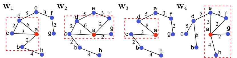
A crucial consequence of the presence of local constraints in weighted networks is illustrated in Fig.1, where we show an example of different networks with the same strength sequence. For a given choice of , in different realizations of the network each node can have different neighbours and different distributions of weights on the links that connect it to those neighbours. In particular, the strength can be more or less concentrated on specific neighbours (a property that is usually quantified by the so-called disparity Serrano et al. (2006)). However, more homogeneous choices of unavoidably result in less concentrated link weights, while more heterogeneous choices of impose more concentrated link weights. This fact will allow us to consider (in Sec. IV) different structural regimes ranging between two extreme limits: a constant (infinite-temperature) strength sequence implying that on average each node is connected to its neighbours in an equally strong way, and a ‘step-like’ (zero-temperature) strength sequence implying an extreme concentration of link weights among a small subset of the nodes. In between these two limits, a certain critical temperature separates a ‘non-condensed’ (high-temperature) phase from a ‘condensed’ (low-temperature) phase featuring the properties of BEC.
II.2 Canonical weighted network ensemble
We first discuss how to implement the strength sequence constraint mathematically in the canonical ensemble (soft constraint) Squartini and Garlaschelli (2017b). Recall that in the traditional canonical ensemble the inverse temperature is the only (scalar) parameter of the canonical probability distribution , conjugate to a certain (scalar) total energy in the corresponding microcanonical ensemble. Explicitly, is the Boltzmann distribution with inverse temperature . By contrast, in our setting the canonical distribution has to depend on an -dimensional vector of parameters, conjugate to the -dimensional constraint which, in turn, defines the microcanonical ensemble. This distribution is found by maximizing the Gibbs-Shannon entropy functional defined in Eq. (1) under the soft constraint
| (4) |
which generalizes the conjugacy condition in Eq. (2). The solution to the maximization problem sees play the role of a vector of Lagrange multipliers coupled to the strength sequence , and is given by Squartini and Garlaschelli (2017b)
| (5) |
where the (network) Hamiltonian is the linear combination of the node strengths, the partition function is a normalization constant, and is the unique parameter value realizing Eq. (4). Note that Eq. (5) has still the form of the Boltzmann distribution, with the important caution that the inverse temperature has been reabsorbed into the Hamiltonian. Therefore, to keep the parallel with the traditional physical situation, in our setting the Hamiltonian should be thought of as the inverse temperature times the energy, and as the inverse temperature times a vector of ‘fields’, each coupled to a different constraint. Clearly, since the probability in Eq. (5) must be dimensionless, the product must be dimensionless as well. In Sec. IV, we will notice that the Hamiltonian can be further reinterpreted as also incorporating a ‘chemical potential’ governing the expected weight of the links in the network Garlaschelli et al. (2013).
Notably, depends on only through . In particular, it gives the same value to any network such that . Explicitly, given the definition of node strength in Eq. (3), the network Hamiltonian can be written for a generic value of as
| (6) |
The partition function can be easily shown Squartini and Garlaschelli (2017b) to be
| (7) |
provided that for all (otherwise, the model admits no solution). The canonical probability distribution therefore factorizes over pairs of nodes as
| (8) |
where
| (9) |
is the probability that the weight of the link between nodes and takes the particular value . Therefore different pairs of nodes are statistically independent in the canonical ensemble (while they are not in the microcanonical one).
Note that is a geometric distribution Squartini et al. (2015b); Squartini and Garlaschelli (2017b) with expected value
| (10) | |||||
(representing the expected weight of the link connecting nodes and ) and variance
| (11) | |||||
As we will discuss in detail is Sec. IV, Eq. (10) has the form of Bose-Einstein statistics, where plays the role of an expected occupation number for the state labeled by nodes and . In an appropriate ‘low-temperature’ regime, BEC can emerge into the model through the divergence of the occupation number for one (possibly degenerate) ‘ground state’ (corresponding to ), while the occupation number for the other states remains finite Park and Newman (2004); Squartini and Garlaschelli (2017b); Garlaschelli and Loffredo (2009). This discussion requires a series of considerations that we leave for later. For the moment, we notice that Eq. (10) allows us to determine the special value corresponding to the given strength sequence . Summing over all nodes , the average value of the strength of node is
| (12) |
whence we can reformulate Eq. (4) as
| (13) |
which fixes the unique parameter value . Notably, this value is also the one that maximizes the (log-)likelihood Garlaschelli and Loffredo (2008); Squartini and Garlaschelli (2017b), i.e.
| (14) |
where, again, is any configuration such that . In general, it is not possible to write explicitly as a function of . However, Eq. (13) or equivalently Eq. (14) can be efficiently solved numerically Squartini et al. (2015b); Squartini and Garlaschelli (2017b) using various algorithms that have been coded for this purpose max ; meh . In any case, a general property (that we will use later) is that for any two nodes and with the same expected strength (), the corresponding parameters and obey the same equation in (13) and are therefore equal. In other words, implies .
Once is calculated, we can plug it back into Eq. (8) to finally obtain the probability distribution
| (15) |
that characterizes the canonical ensemble entirely. For practical purposes, can be inserted into Eq. (9) to obtain the link weight probability , from which several expected network properties can be calculated very directly. For instance, besides the expected link weight , we can calculate the probability that nodes and are connected by a link, irrepective of the weight of the latter, as follows:
| (16) | |||||
where denotes the Heaviside step function, defined as if and if . Note that, if and belong to the condensed state where the expected link weight diverges (), then they become deterministically connected, i.e. . By contrast, non-condensed states have , , and . The analogy with BEC will be discussed in much more detail in Sec. IV.
Besides the structural properties, one of the key quantities that we will need in order to determine EE (or the lack thereof) is the resulting canonical entropy , obtained by inserting Eq. (15) into Eq. (1):
| (17) | |||||
Note that the calculation of the canonical entropy of the entire weighted network ensemble only requires the knowledge of the probability of one generic network with strength sequence , which is in turn directly calculated through Eq. (15).
II.3 Microcanonical weighted network ensemble
We now come to the microcanonical ensemble. Its governing probability distribution can be obtained by maximizing the Gibbs-Shannon entropy functional in Eq. (1) under the hard constraint
| (18) |
that applies to each network realized (with positive probability) in the set . The solution is obviously the uniform probability distribution
| (19) |
where is the number of networks for which the hard constraint in Eq. (18) is realized. An implicit assumption throughout this paper is that the particular strength sequence is graphic, i.e. it can be realized by at least one network, so that . In this case as well, the (microcanonical) entropy is obtained by inserting Eq. (19) into Eq. (1):
| (20) | |||||
which is also known as Boltzmann entropy. Note that has the same meaning as in Eq. (17), therefore both the canonical and microcanonical entropies are equal to minus the log of the corresponding probability, evaluated in any state realizing the hard constraint in Eq. (18).
Note that, although the derivation of is formally much more direct than that of in the conjugate canonical ensemble, its explicit calculation is more challenging, as it requires the combinatorial enumeration of all the weighted networks with strength sequence (as a side remark, it is precisely the local nature of that makes the calculation of daunting). Here, we will employ a recently proposed saddle-point asymptotic formula, for a generic discrete system under a -dimensional vector of effective (see Sec. I.3) constraints, for the number of microcanonical configurations Squartini and Garlaschelli (2017a). The formula uses only conjugate canonical quantities, namely the canonical entropy and the covariance matrix among the constraints in the canonical ensemble, and reads Squartini and Garlaschelli (2017a)
| (21) |
where are the eigenvalues of . The symbol indicates a quantity with a finite limit when divided by as , i.e. is asymptotically of the same order as . Note that, since covariance matrices are positive semidefinite, for all . Moreover, since the constraints are assumed to be non-redundant, then for all Squartini and Garlaschelli (2017a) (if some of the constraints were redundant, there would be certain zero eigenvalues rendering the above equation inapplicable; that is why the formula should be applied to a maximal set of non-redundant constraints). Finally, if these eigenvalues grow sufficiently fast as , then the product on the right hand side becomes irrelevant, in which case the knowledge of and is enough in order to characterize the asymptotics of .
In our setting where and (node strengths are all mutually independent as it is not possible to guess any individual node strength from the knowledge of the other ones), we calculate the entries of as
| (22) | |||||
where is given by Eq. (7). An explicit calculation gives
| (23) | |||||
for the diagonal entries (i.e. the variances of the constraints) and
| (24) | |||||
for the off-diagonal entries (i.e. the covariances between distinct constraints).
We finally obtain
where we have used . Note that the eigenvalues are positive, the node strengths being linearly independent constraints Squartini and Garlaschelli (2017a). In principle, in order to compute (the leading term of) Eq. (II.3) explicitly, we need to specify a value for , calculate the resulting matrix , and the eigenvalues of the latter. However, in Sec. III we show that the knowledge of the diagonal elements of the covariance matrix is enough for our purposes. This result is then used in Sec. IV when we consider specific choices of .
III Equivalence and nonequivalence of weighted network ensembles
In this section we use the knowledge of the canonical and microcanonical probability distributions derived in the previous section in order to establish two criteria for the equivalence of ensembles of weighted networks, namely the one based on the vanishing of the relative entropy density between the two distributions Touchette (2015) and the traditional one based on the vanishing of the canonical relative fluctuations of the constraints Gibbs (1902).
III.1 Relative entropy density
As we have anticipated, EE can be stated mathematically using three different notions, namely thermodynamic, macrostate and measure equivalence Touchette (2015). These definitions turn out to be, under mild assumptions, essentially equivalent Touchette (2015). Here, we use the definition in the measure sense, which has been recently formulated explicitly for binary network ensembles Squartini et al. (2015a); Garlaschelli et al. (2016); Roccaverde (2019); Squartini and Garlaschelli (2017a) and is based on the vanishing of a suitable relative entropy density between the microcanonical and canonical probability distributions. Our calculations generalize those results to the case of weighted networks, for which measure equivalence has not been studied yet.
In general, the relative entropy (or Kullback-Leibler divergence) between two distributions and , both having support over a discrete set of configurations in analogy with Eq. (1), is defined as
| (26) |
and quantifies ‘how far’ the distribution is from the reference distribution Kullback and Leibler (1951). When and represent the microcanonical and canonical distributions respectively, it can be shown Squartini et al. (2015a); Squartini and Garlaschelli (2017a) that reduces to the difference between the canonical and microcanonical entropy, which can be both estimated on a single configuration realizing the hard constraint (as we have indeed shown in the previous section for our weighted network model). Moreover, its calculation asymptotically requires only the canonical covariance matrix between the constraints.
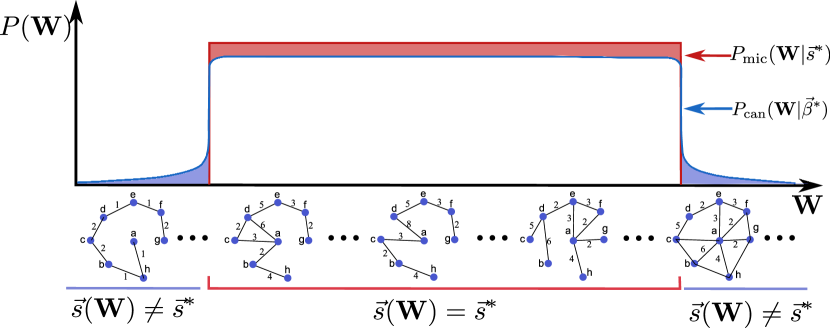
We are now going to see how these general results apply to our specific case. A visual illustration of the idea behind measure equivalence for our ensembles of weighted networks with given strength sequence is provided in Fig. 2. Following Eq. (26), the relative entropy between and is defined as
| (27) | |||||
By inserting Eq. (19) into Eq. (27) and using the fact that has the same value for any network matching the hard constraint , we confirm that can be estimated pointwise on as
| (28) |
Moreover, using Eqs. (17) and (20), we also confirm that it reduces to the entropy difference
| (29) |
Now, Eq. (II.3) immediately allows us to obtain
| (30) |
which depends only on the eigenvalues of the canonical covariance matrix , whose diagonal and off-diagonal entries are given in Eqs. (23) and (24) respectively.
The definition of measure equivalence is the vanishing of the relative entropy density, i.e. of the ratio , in the thermodynamic limit Touchette (2015). Explicitly, EE in the measure sense corresponds to
| (31) |
or equivalently Squartini and Garlaschelli (2017a)
| (32) |
where denotes a quantity that, if divided by , vanishes as . Equation (29) allows us to understand the above definition of macrostate EE as follows. The microcanonical entropy is the logarithm of the number of accessible configurations under hard constraints, while the canonical entropy is the logarithm of the corresponding ‘effective’ number of configurations under soft constraints. EE requires that, as increases, the typical configurations of the system under the two ensembles become the same, i.e. that the (effective) numbers of configurations in the two ensembles become closer to each other. This cannot happen if, as we keep adding one more unit to the system, the difference between the two entropies (i.e. the relative entropy ) keeps increasing by an arbitrary amount. The criterion in Eq. (31) establishes that if the entropy difference per node, i.e. , does not vanish as diverges, then the two ensembles cannot be equivalent.
Equation (32) implies that, in order to assess whether the system is under EE, we do not need the exact value of , but only its leading order with respect to . Then from Eq. (30) we see that, since the term is at most of the same order as , the presence of does not affect ensemble (non)equivalence:
| (33) |
So, in order to check whether Eq. (32) holds, it is ultimately enough to check whether
| (34) |
On the other hand, since our hypothesis of non-redundant constraints implies for all (as discussed in Sec. II.3), we see that the contribution of the term to the relative entropy in Eq. (30) is at most . So if grows faster than then Eq. (30) reduces to the stronger result
| (35) |
i.e. the leading term of the relative entropy (not only its leading order) can be calculated exactly from (throughout this paper, the symbol “” indicates that the leading term of and is asymptotically the same, i.e. the two quantities differ by a quantity that vanishes if divided by either or as ). Depending on the regimes considered later on in the paper, different techniques for calculating (the leading order of) the determinant of the covariance matrix can be used. We will discuss these techniques when needed, and refer to the Appendix for explicit calculations. We will show that, except in a certain zero-temperature limit, the conditions ensuring Eq. (35) are met and the leading order of the relative entropy can be calculated exactly.
III.2 Relative fluctuations of the constraints
We now consider the relative fluctuations of the constraints, whose behaviour in the thermodynamic limit is, historically, the traditional criterion used to check whether statistical ensembles are equivalent Gibbs (1902). In the standard situation, where the canonical and microcanonical ensembles are defined through a single scalar constraint on the total energy , the relative fluctuations are captured by a single scalar quantity representing the ratio of the canonical standard deviation of the energy to the mean energy itself. EE is then associated with the vanishing of as . In statistics, is called the coefficient of variation of the random variable with expected value and variance
In the case of networks with local constraints, there are coefficients of variation to consider. They have been calculated for both the binary and the weighted versions of the configuration model Squartini et al. (2015b). In extreme summary, those results show that, in the binary case (where there is a constraint on the degree for each node ), an upper bound for the relative fluctuation can been established. By contrast, in the weighted case (corresponding to the model considered here with a constraint on the strength for each node ), the value becomes a lower bound for the relative fluctuation Squartini et al. (2015b). Those results have two implications.
First, in the binary case the only regime for which general conclusions can be drawn about the vanishing of the relative fluctuations is the so-called dense regime where the expected degree of all nodes diverges, hence . In the opposite sparse regime where the average degree of all nodes is finite, we only have a finite upper bound for the relative fluctuations, but their actual value depends on the specific network. In general, however, the decreasing behaviour of the upper bound for the relative fluctuations in binary networks with increasing degrees is opposite to that of the relative entropy density, which increases as the expected degree increases Squartini et al. (2015a); Garlaschelli et al. (2016); Roccaverde (2019).
Second, in the weighted case we have a somewhat opposite situation where we can only conclude that, in the sparse regime where the expected strengths are finite (apart from possible hubs), the relative fluctuations do not vanish. By contrast, in the dense case where the expected strengths diverge, the relative fluctuations can in principle pick any value. Confusingly, even if in the weighted case the lower bound for the relative fluctuations of the strengths goes to zero for nodes with diverging strength , previous results seem to indicate that the realized value of in networks with heterogeneous strength sequence actually increases for higher Squartini et al. (2015b). This behaviour suggests that weighted networks, due to the many possible ways in which weight can accumulate on links, can behave very differently from binary networks. This observation requires further research and strengthens our motivation for studying the relative fluctuations in weighted networks in different scenarios (ranging from homogeneous to heterogenous concentrations of link weights), in conjunction with the relative entropy and, in general, ensemble (non)equivalence.
Using Eq. (23), we can immediately calculate the standard deviation of each constraint around its expected value as
| (36) | |||||
The relative fluctuation of the strength is therefore
| (37) |
Since for all , we have , showing that is indeed a lower bound for . When studying the asymptotic behaviour of the relative fluctuations in the thermodynamic limit, we will be interested in whether the limit
| (38) |
is zero (vanishing relative fluctuations) or positive (nonvanishing relative fluctuations) for each node .
IV BEC in weighted networks
In physical systems composed of bosons, i.e. particles obeying Bose-Einstein statistics, BEC is a phase transition whereby, below a certain critical temperature, a finite fraction of the total number of particles condenses in the ground state, i.e. the state with lowest energy (or more generally in a finite number of states with lowest energy). BEC was theoretically predicted by Satyendra Nath Bose and Albert Einstein in 1924 Einstein (1924), and it has since then been observed in various physical systems. Models of BEC have been studied in different statistical ensembles in the standard case with only global constraints (total energy and/or total number of particles) Navez et al. (1997); Holthaus et al. (1998); Mullin and Fernandez (2003); Chatterjee and Diaconis (2014); Tarasov et al. (2015); Crisanti et al. (2019). Although the detailed phenomenology exhibited by these models depends on the choice of the energy and the structure of the interactions, it is generally found that EE breaks down in the condensed (low-temperature) phase, as signalled by nonvanishing relative fluctuations of the constraints.
In this Section, we are going to show that a form of BEC, even if quite different from that found in more traditional physical settings, can also appear in our ensembles of weighted networks. The possible onset of BEC in our system creates an ideal situation where an EE-breaking phase transition can be studied in combination with an additional and unrelated mechanism for the breakdown of EE, i.e. the presence of local constraints, which is always active in both the condensed and the non-condensed phases. To illustrate our results, we first make some important clarifications in order to establish a rigorous link from weighted network ensembles to Bose-Einstein statistics and then study the different phases of the model.
IV.1 Bose-Einstein statistics in weighted networks
As we have already recalled, weighted networks with a constraint on the strength sequence obey Bose-Einstein statistics, as opposed to binary networks that obey Fermi-Dirac statistics Park and Newman (2004); Garlaschelli and Loffredo (2009); Garlaschelli et al. (2013). Indeed, inserting Eq. (6) into Eq. (5) we get the probability of a configuration for a gas of free particles in the grandcanonical ensemble222In the grandcanonical ensemble, both the total energy and the total number of particles are treated as soft constraints. With respect to the canonical ensemble, the appearance of the number of particles as an additional soft constraint requires the introduction of an extra Lagrange multiplier, the chemical potential. Interestingly, in the context of BEC a fourth (so-called ‘Maxwell’s Demon’) ensemble has also been introduced where the total number of particles is soft while the total energy is hard Navez et al. (1997)., where the pair labels an energy state, the weight is the number of particles in that state (occupation number), and the sum can be interpreted as
| (39) |
In the latter expression, represents the energy of the state, is the inverse temperature, and is the chemical potential (required to fix the same expected overall number of particles for all values of ) Garlaschelli et al. (2013). Indeed, as we discussed in Sec. II.2, in our setting the energy and temperature (and in this case, the chemical potential as well) are all reabsorbed into . Therefore we can interpret the link weight as the number of ‘elementary particles’ of weight, i.e. the number of quanta of unit weight, populating the link between nodes and Park and Newman (2004); Garlaschelli and Loffredo (2009). The total number of such particles in the system is the total weight of all links in the network:
| (40) |
The ‘weighted’ property , which leads to Eqs. (7), (8) and (9), corresponds to the possibility that the same state (pair of nodes) is occupied by indefinitely many particles (subject to the average number dictated by the chemical protential), which is a property of bosons. By contrast, in binary networks one has to impose , which is a property of fermions Park and Newman (2004). An extensive treatment of the role of chemical potential and temperature in binary networks can be found in Garlaschelli et al. (2013). Here, to properly interpret what the weighted model is doing, we should give a series of clarifications.
First, we should make a clear distrinction beween the ‘units’ of our system (i.e. the nodes of the network) and the ‘particles’ of weight that, as a formal analogy, can be interpreted as populating the links of the network. The former are the real constituents of our physical system, while the latter are a mathematical abstraction used to represent the nature of the interactions (links) between such constituents. If we imagine doubling the size of our network, we should imagine doubling the number of nodes: indeed, we can imagine the network ‘growing in size’ by adding one single node at a time, but we cannot imagine adding one single pair of nodes at a time, without actually adding new pairs. One should also not be tempted to regard node pairs as the fundamental units by the fact that, mathematically, the variables involving different pairs of nodes are independent random variables: actually, this only occurs in the canonical ensemble and would in any case not be true for more general choices of the constraints. Moreover, even the independent node pairs in the canonical ensemble cannot be assigned independent values of the parameters, since there are only parameters corresponding to the Lagrange multipliers attached to each node. Explicit (and strong) consequences of this fact will be illustrated precisely in the context of BEC. Therefore the physical size of our system is , and this is why in Eq. (31) we defined the relative entropy density as the relative entropy divided by in the first place. How the total weight varies with the system size depends on a specific property, i.e. on how we make the entries of (and the resulting value of ) scale with . For instance, we may choose to be in the sparse regime where remains finite as , or in the dense regime where diverges as . As we show below, the latter is the relevant case for BEC to emerge.
Second, we stress that, irrespective of the above, we always consider a hard number of nodes, and this is why we compare (only) the canonical (soft value of ) and microcanonical (hard value of ) ensembles of networks, both for fixed (which sets the dimension of ). We do not consider the grandcanonical ensemble of network configurations where is soft. The grandcanonical ensemble introduced in the aforementioned analogy with systems of bosons is a different one; it may be denoted as an ensemble of weight quanta in a network with fixed and originates from the fact that the Hamiltonian in Eq. (6), and consequently the total link weight (not ) in Eq. (40), is a fluctuating quantity in the canonical ensemble of network configurations. The fluctuations in the (rescaled) energy (canonical ensemble of network configurations) are seen as fluctuations in the particle number (grandcanonical ensemble of weight quanta) in the Bose-Einstein analogy. Fluctuations in the particle number have been the subject of many studies in the literature on BEC Navez et al. (1997); Holthaus et al. (1998); Mullin and Fernandez (2003); Chatterjee and Diaconis (2014); Tarasov et al. (2015); Crisanti et al. (2019). Note that, in both canonical and microcanonical ensembles, the individual link weights are fluctuating quantities, despite the fact that the total link weight is constant in the microcanonical ensemble. Therefore the numbers of ‘weight particles’ of individual links fluctuate in both ensembles.
Third, while we necessarily discuss the (non)equivalence of the canonical and microcanonical ensembles in the thermodynamic limit , the total weight can (and, across the canonical ensemble, will in any case) be arbitrarily large even for finite . Indeed, the phase transition that we are about to discuss (namely, BEC) does not per se require the limit , while it definitely requires the limit . Abstractly, these two limits (and the associated phenomena of EN and BEC respectively) may appear as mathematically unrelated. However, in practice they are physically related once the scaling of with is specified. In particular, we are going to show that, in order to observe BEC, we need be in a dense regime where . This ensures that, when taking the thermodynamic limit in order to study ensemble (non)equivalence, we are automatically implying so that we can check for BEC at the same time.
Last, we recall that has to be dimensionless in order to ensure that the probability is a number. Therefore, since is dimensionless, so are and . In turn, this implies that both sides of Eq. (39) must be dimensionless. On the other hand, when modelling a real system, the ‘energy’ may represent any physical ‘cost’ associated to the link between nodes and (more precisely, it represents the cost of reinforcing by a unit of weight) and may therefore carry its own unit of measure (e.g. it may depend on some distance between nodes and ). Necessarily, the chemical potential carries the same units as the energy. As for the ‘temperature’ , it may be chosen to be dimensionless as it merely represents a control parameter (this is the choice that we will make later); alternatively, it may carry the same units of the energy if it is useful that temperature and energy live on the same scale. Irrespective of this choice, in our setting the ‘Boltzmann constant’ is simply a constant that takes care of all dimensional units of measure and makes the ratio on the right hand side of Eq. (39) dimensionless.
IV.2 Core-periphery networks
With the above clarifications, we can finally go back to our model. In the traditional physical situation, in the canonical ensemble the energy of each state is a constant and the temperature can be varied. Clearly, is independent of , while the chemical potential is chosen, as a function of temperature, in order to realize the correct (-independent) expected total number of particles for all values of . In this ‘direct problem’, every state will therefore have an expected occupation number governed by , and . In our ‘inverse’ setting, and are instead reabsorbed into , which in turn is induced by the chosen value of the strength sequence (rather than the other way around). We should therefore regard and as -dependent, while remains -independent. This means that the chemical potential should be such that
| (41) |
BEC emerges when, below a certain critical temperature , the occupation number of the state with minimum energy (ground state), or of a finite number of states with lowest energy, becomes so large that it reaches a finite fraction of the total number of particles. Clearly, this requires the existence of at least two different energy levels (the ground state and at least one ‘excited’ state). Therefore the simplest way to obtain BEC in our model is by considering a strength sequence of the form
| (42) |
i.e. by partitioning the nodes into two classes, which we call core and periphery: the core has a finite number
| (43) |
of nodes, each having a ‘large’ strength , while the periphery has an extensive number
| (44) |
of nodes, each having a ‘small’ strength . What we mean precisely by ‘small’ and ‘large’ will be clarified below. For the moment, we notice that the BEC phase () corresponds to picking a ‘condensed’ value of such that, in the thermodynamic limit, the core takes up a finite fraction of the total weight of all links in the network, despite having a finite size. In particular, in the zero-temperature limit all the total weight is in the core. By contrast, the non-condensed phase is one where is such that no individual link receives a finite fraction of . In particular, the infinite-temperature limit should be such that the energy difference between ground and excited states becomes ineffective, i.e. . The different phases can be efficiently monitored by introducing a temperature-dependent order parameter , as we show below.
We stress that, since we are ultimately interested in the relative fluctuations of the canonical constraints and in the relative entropy that can be asymptotically calculated purely from canonical quantities according to Eq. (33), practically we only need to study the canonical ensemble. The only check we need to make is that, whenever we speak of the system being in a certain ‘phase’, this statement does not depend on the particular ensemble. In other words, we need to show that the order parameter has always the same value in the canonical and microcanonical ensembles.
Before studying the individual phases, let us make some general considerations, valid for all values of . We first find the value of corresponding to the value of in Eq. (42). As we mentioned, implies , therefore the entries of take only two values and such that
| (45) |
These values solve the equations in (13), which here reduce to the two independent equations
| (46) | |||||
| (47) |
where we have defined
| (48) |
as the expected link weight between any two nodes in the core (),
| (49) |
as the expected link weight between any two nodes in the periphery (), and
| (50) | |||||
as the expected link weight between any node in the core and any node in the periphery ( and or and ). Note that implies .
Now, solving Eqs. (46) and (47), we obtain the explicit values of and appearing in Eq. (45):
| (51) |
Also note from Eq. (50) that
| (52) |
Also, using Eq. (16) we can define
| (53) |
as the probability that a link exists (irrespective of its weight) between any two core-core () or any two periphery-periphery () nodes, and
| (54) |
as the probability that a link exists (irrespective of its weight) between a core node and a periphery node.
From Eq. (39), we notice that the existence of the two values above for the entries of implies that there are three energy levels, associated with the energies
| (55) | |||||
| (56) | |||||
| (57) |
where (we recall that all energy values are finite and independent of both and ). The appearance of three distinct energy levels out of just two values of the fundamental Lagrange multipliers confirms the interpretation that the true units of the system are the nodes and not the node pairs: it would indeed be impossible for our system to exhibit exactly two energy states, or in general to engineer an arbitrary number of energy states for the node pairs, since the only arbitrary values are those that can be attached to nodes, not to node pairs. Also note that all the three levels above are degenerate: the pairs of nodes in the core have the same expected link weight and energy , the pairs of nodes in the periphery have the same expected link weight and energy , and the pairs of nodes across core and periphery have the same expected link weight and energy . Therefore the ground state has energy and degeneracy . These degeneracies are dictated by the numbers of nodes in the two sets and cannot be assigned arbitrarily.
The occupation number of the ground state (with energy ) coincides with the expected weight of all links between core nodes (total ‘core-core’ weight):
| (58) |
Similarly, the occupation number of the first excited state (with energy ) coincides with the expected weight of all links between nodes across core and periphery (total ‘core-periphery’ weight):
| (59) |
Finally, the occupation number of the second excited state (with energy ) coincides with the expected weight of all links between periphery nodes (total ‘periphery-periphery’ weight):
| (60) |
By writing as the sum of its core-core, core-periphery and periphery-periphery components, we get
| (61) | |||||
Using Eq. (41), the total weight can also be expressed as
| (62) |
which, through Eqs. (46) and (47), indeed reduces to Eq. (61).
We stress again that the chemical potential appearing in Eqs. (55), (56) and (57) plays the role of a global Lagrange multiplier ensuring that, for all values of , the total expected weight is . Note that the -independence of allows us to conclude immediately that its value should be of order
| (63) |
because, in particular, in the non-condensed phase all the individual link weights , must be finite by definition. As we have anticipated, this result ensures that in the thermodynamic limit () we automatically have , so that we can study ensemble (non)equivalence and BEC simultaneously, thereby ‘physically’ connecting two otherwise mathematically unrelated limits. We also note that, irrespective of temperature, the network is always in the dense regime. We can therefore introduce the average expected link weight
| (64) |
which is a -independent, finite parameter of our model, controlling the overall link weight in the network. Clearly,
| (65) |
It is good to remark again that, in our ‘inverse’ problem (construction of the conjugate canonical and microcanonical ensembles), the parameters of the model are the values of the constraints, which here reduce to the two (diverging when ) numbers . However, to allow consistent comparisons for different temperatures, not all strength sequences are allowed, but only those that can be obtained from one another by varying . In particular the values have to be specified for each value of and be such that the total weight is always . Indeed Eq. (62) shows that only two of the three quantities , are independent. By contrast, the traditional ‘direct’ problem in physics sees the three energies and (which do not depend on ) as the parameters of the model, plus either or the chemical potential . However, Eq. (57) shows that , indicating only two independent values of the energy (say ), as a result of the fact that there are only two types of nodes. Moreover, we may set the minimum energy without loss of generality, because any overall energy shift can be reabsorbed into the chemical potential. We can therefore rename the only remaining independent value of the energy as , and similarly . Using these replacements into Eqs. (55) and (56), and combining the two equations, we get
| (66) |
which is a convenient expression for solving the ‘direct’ problem. Rearranging, we obtain
| (67) |
and, using Eqs. (51) and (53),
| (68) | |||||
which shows how the energy difference between periphery-periphery () and core-core () states is related to the corresponding connection probabilities and expected link weights . Therefore the most compact way of parametrizing the direct problem is by specifying only the two finite, positive and -independent numbers and , and explore the resulting network properties by finding (as a function of , and ) and varying as a control parameter. This will indeed allow us to easily explore the different (high- and low-temperature) phases consistently.
In our model, BEC occurs below a critical temperature such that a finite fraction of the total weight condenses in the core, which remains of finite size (i.e. of a finite number of nodes) even when the size of the whole network diverges. This corresponds to requiring that, as , remains finite as dictated by Eq. (43), diverges, and takes up a finite fraction of . Rigorously, we can define this fraction (for finite ) as
| (69) |
and use it to introduce the order parameter as
| (70) |
We can then define the BEC phase as a phase emerging below a certain critical temperature such that
| (71) |
By contrast, the non-BEC phase is such that
| (72) |
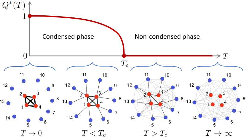
A visual anticipation of the qualitative behaviour that our system will exhibit is provided in Fig. 3.
In conjunction with BEC, we will investigate ensemble (non)equivalence. Therefore, in each phase of the model we will consider the relative entropy between the microcanonical and canonical ensembles and the relative fluctuations of the constraints. The criterion for measure equivalence is based on the relative entropy in Eq. (33), and useful techniques for the calculation of the determinant of the covariance matrix in each phase are provided in the Appendix. Clearly, from Eqs. (23) and (45) we see that the diagonal entries of take two possible values:
| (73) |
where
| (74) | |||||
Recalling Eq. (7), we remark that the canonical entropy can be easily calculated from Eq. (17) as the following sum of five terms:
| (75) | |||||
while the microcanonical entropy is in general hard to compute, as it requires an explicit enumeration. However, its leading order can be obtained combining Eqs. (II.3) and (75).
The relative fluctuations of the constraints take the form
| (76) |
where, from Eq. (37),
Therefore in the thermodynamic limit the relative fluctuations of the constraints, as defined in Eq. (38), take only the two possible limiting values
| (78) |
where
| (79) |
Armed with the above general results, we can now study each phase in detail.
IV.3 Non-condensed phase
Let us start from the non-BEC phase (). We first consider the finite-temperature case () and then the infinite-temperature limit (). As all the interesting phenomenology (in terms of both BEC and EN) occurs in the thermodynamic limit , we look for the asymptotic behaviour of all quantities in that limit.
IV.3.1 Finite (supercritical) temperature:
Since, by definition, when there is no concentration of ‘particles’ of weight on any of the links, all the expected link weights must be separately finite, i.e. , and are all . Consequently, from Eqs. (53) and (54) we see that all the connection probabilities , and are strictly smaller than one, i.e. missing links can occur anywhere in the network. Using this fact into Eqs. (46), (47), (58), (59) and (60), and using Eqs. (43) and (44), we immediately get the strength of nodes in the core, i.e.
| (80) | |||||
and in the periphery, i.e.
| (81) | |||||
Similarly, for , we get
| (82) | |||||
| (83) | |||||
| (84) |
from which we see that in this phase the total weight is essentially all in the periphery, i.e.
| (85) | |||||
| (86) |
We stress that the above result does not mean that the core is empty or that there are no connections between core and periphery. Rather, it indicates that the total weight of all core-core and core-periphery connections is asymptotically negligible with respect to the total weight located inside the periphery, simply because the number of periphery-periphery node pairs dominates the number of core-periphery and core-core pairs. In particular, the finite parameter can take an arbitrarily large value, without ‘moving’ the (finite and positive) value of the average link weight . All positive values of are therefore allowed. By contrast, is forced to take (to leading order) only the value .
Using Eqs. (81), (83) and (84), we write the order parameter as
| (87) | |||||
confirming the definition of non-condensed phase in Eq. (72) and showing that, since both and have by construction the same value in the canonical and microcanonical ensemble, the order parameter must be zero in both ensembles, for all values of . Therefore, whenever one ensemble is in the non-condensed phase, the other ensemble is the non-condensed phase as well. Importantly, this allows us to refer to the conjugate canonical and microcanonical ensembles ‘in the non-condensed phase’ consistently.
To solve the ‘inverse’ problem, we use Eqs. (51) and (52) and invert Eqs. (80) and (81) to get
| (88) | |||||
and
| (89) | |||||
Then, subtracting Eq. (88) from Eq. (89), we get
| (90) | |||||
Equations (88) and (90) express as a function of the two (diverging) constraints , or equivalently as a function of the finite parameters , which have to be specified for all values of .
To solve the ‘direct’ problem, we first note an important consequence of Eq. (86): in the large limit, and are independent of temperature. Indeed, using Eq. (81) and (86) into Eq. (88), we get asympotically
| (91) |
and, using Eq. (67),
| (92) |
When inserted into Eq. (66), the above expressions allow us to directly obtain the chemical potential as
| (93) | |||||
As anticipated, the above result provides the solution to the direct problem in terms of the two finite constants and , and allows us to explore the model by varying throughout the non-condensed phase .
We now consider ensemble (non)equivalence. Inserting Eqs. (80) and (81) into Eq. (74), we obtain the variance of the strength of nodes in the core, i.e.
| (94) | |||||
and in the periphery, i.e.
| (95) | |||||
As we show in Appendix A.1, it is possible to show that the leading term of the determinant of the covariance matrix in this non-condensed phase is
| (96) |
Using Eqs. (74), (94) and (95) we obtain
| (97) | |||||
Inserting this result into Eq. (96), we find
| (98) |
showing that the determinant is dominated by the diagonal entries of . Taking the logarithm, we obtain
| (99) |
which, when compared with Eq. (34), shows that the system is under ensemble nonequivalence. We note that the scaling of ensures that Eq. (35) holds, so the leading order of the relative entropy can be calculated exactly as
| (100) |
where we have used Eqs. (94) and (95) into Eq. (96). The above result is in line with the scaling of the relative entropy found in the case of binary networks with a constraint on the node degrees in the dense regime Squartini et al. (2015a); Garlaschelli et al. (2016); Roccaverde (2019). Another similarity between the two models is the order of the canonical entropy:
| (101) |
which can be easily seen from Eq. (75) using and , as found in Eqs. (80), (81), (88) and (90). Then Eq. (II.3) also implies
| (102) |
Note that, even if the relative entropy is subleading with respect to the canonical and microcanonical entropies, it is still superextensive in the number of units of the system, thereby breaking ensemble equivalence as in binary networks with fixed degrees. Therefore the result in Eq. (99) is another observation, for the first time in weighted networks, of the fact that ensemble equivalence can be broken by the presence of an extensive number of local constraints, even away from phase transitions.
Coming to the relative fluctuations of the constraints, we see from Eqs. (IV.2) and (79) that
| (103) | |||||
and
| (104) |
We therefore observe that in the non-condensed phase the decay of the relative fluctuations of each constraint is of the same order as generally observed for the global constraint (total energy) in a system with short-range interactions away from phase transitions. However, while in the traditional situation the vanishing of the relative fluctuations implies that the relative entropy is subextensive and that the relative entropy density vanishes in the thermodynamic limit (as discussed in Sec. I.3), here the relative entropy density does not vanish and the ensembles are not equivalent. Therefore we find that, in systems with an extensive number of local constraints, the vanishing of even all the relative fluctuations does not ensure ensemble equivalence.
IV.3.2 Infinite temperature:
The extreme regime of the non-condensed phase is the infinite-temperature case, which can be explored by taking the limit in the solution to the ‘direct’ problem provided by Eq. (93). In such a limit, Eq. (39) implies that and converge to the same value given by
| (105) |
Then, through Eqs. (48), (49), (50), (53) and (54), we get
| (106) | |||||
| (107) |
i.e. all node pairs have the same expected link weight and connection probability given by
| (108) |
This is the characteristic situation in the infinite-temperature limit of Bose-Einstein statistics, where each particle is equally likely distributed across all energy levels. Here, this situation translates in the graph becoming completely homogeneous: the distinction between core and periphery disappears as the finite difference between energy levels becomes entirely dominated by the diverging temperature. The expected strength of every node has the same value :
| (109) |
i.e. the strength sequence becomes a constant vector.
Clearly, the above result does not change the value of the order parameter in Eq. (87):
| (110) |
Similarly, the final results in eqs. (99) and (104) about the simultaneous breakdown of ensemble equivalence and the vanishing of all relative fluctuations carry over to the infinite-temperature limit, so in principle we do not have to further discuss this case. However, the fact that the strength sequence becomes a constant vector allows us to calculate many of the properties of the model exactly, so this example is a very transparent and instructive one. It is therefore worth considering it in some more detail, also because some of the following results will be useful in the (much less trivial) zero-temperature limit as well.
In particular, Eqs. (105) and (109) imply that Eqs. (23) and (24) can be rewritten as
| (111) |
for all and
| (112) |
for all respectively. In Appendix A.2 we show that the above expressions can be used to calculate the determinant of exactly as
| (113) |
from which we confirm, without having made the approximation in eq. (96), that
| (114) |
and that
| (115) |
Clearly, Eqs. (101) and (102) hold in this limit as well:
| (116) |
IV.4 Condensed phase
We now consider the BEC phase . We first derive general results and then discuss the finite-temperature case and the zero-temperature limit separately.
By the definition in Eq. (71), the condensed phase must be such that a positive fraction of the total weight lies in the core, i.e. (to leading order)
| (119) |
which necessarily means
| (120) |
and , i.e. the core does not have missing links (the presence of core-core links is no longer a random event, while the weight of such links is still a random variable). As expected, BEC corresponds to the divergence of , and we now see that the speed of this divergence is of order in our model. For convenience, we may define
| (121) |
which is finite and positive, so that
| (122) |
Combining Eqs. (50) and (120) we see that
| (123) |
which inserted into Eq. (61) shows that, to leading order,
| (124) |
an expression that relates the finite parameters of the model with each other in the condensed phase. Therefore we see from Eq. (119) that
| (125) |
and
| (126) |
Inserting Eq. (125) into Eq. (123) yields
| (127) |
and
| (128) |
The above expressions show that neither nor diverge, indicating that BEC occurs only in the ground state and that and , i.e. there can be missing links in the periphery and between core and periphery. Moreover, we see that is subleading with respect to both and : although individual core-periphery links have an expected weight larger than the expected weight of individual periphery-periphery links, the number of core-periphery links is of smaller order with respect to the number of periphery-periphery links, and as a result the total weight of all core-periphery links is of smaller order as well.
To obtain to leading order, we use Eqs. (46) and (47):
| (129) | |||||
| (130) | |||||
Now, combining the above expressions, we see that the order parameter defined in Eq. (70) can be written as
| (131) | |||||
Besides quantifying the order parameter, the above calculation shows that, since the value of only depends on the values of and (which by construction are the same in the canonical and microcanonical ensembles), whenever one ensemble is in the BEC phase, the other ensemble is the BEC phase as well, for all temperatures . As for the non-condensed, this allows us to refer to the conjugate canonical and microcanonical ensembles being ‘in the same phase’ consistently. Inverting Eq. (131), we can also express the parameter in terms of the order parameter as follows:
| (132) |
The ‘inverse’ problem is solved by inverting Eqs. (129) and (130) and using them into Eq. (51) to get
| (133) | |||||
| (134) | |||||
The above equations solve the inverse problem by expressing as a function of the constraints , which can in turn be expressed either in terms of the finite parameters and or in terms of and the temperature-independent parameter .
Again, the ‘direct’ problem requires finding the chemical potential as a function of , and . From Eq. (66) we get
| (135) | |||||
We now consider the variance of the constraints. Inserting Eqs. (120), (125) and (127) into Eqs. (74), we immediately see that
| (136) | |||||
| (137) |
IV.4.1 Finite (subcritical) temperature:
In this regime we have
| (138) |
which, as clear from Eqs. (125) and (127), implies
| (139) | |||||
| (140) |
where both quantities are . Using these results, it is possible to show (see Appendix A.3) that the leading term of the determinant of the covariance matrix between the constraints is
| (141) |
implying
| (142) |
which is the same scaling found in Eq. (99) for the non-condensed phase. The criterion for measure equivalence in Eq. (34) is again violated, showing that ensemble equivalence does not hold in the condensed case as well. The leading term of the relative entropy can still be calculated exactly from Eq. (35) and is the same as the one found in Eq. (100) for the non-condensed phase:
| (143) |
Similarly, the canonical entropy is still of order , as can be seen by inserting Eqs. (129), (130), (133) and (134) into Eq. (75). We therefore retrieve
| (144) | |||||
| (145) |
Coming to the relative fluctuations, from Eqs. (IV.2), (79), (136) and (137) we obtain
| (146) | |||||
| (147) |
The above result can be interpreted as follows. The term in Eq. (37) is an inverse participation ratio, taking values in the range and quantifying the inverse of the effective number of link weights contributing to the strength of node Squartini et al. (2015b). Here, for a node in the core, there is a finite number of dominant link weights, each equal to , while the remaining weights are of smaller order. Taking the thermodynamic limit, these dominant weights lead to the value for in Eq. (146). By contrast, for a node in the periphery, all the expected link weights are of the same order, so the inverse participation ratio, and consequently the value of in Eq. (147), vanishes. It should be noted that, even if the expected strength of the core nodes is much bigger than that of the periphery nodes, the relative fluctuations of the core nodes do not vanish, while those of the peripheral nodes do.
The fact that BEC occurs necessarily among the core nodes confirms that the units of the system are the nodes, and not the node pairs: the ‘ground state pairs’ are necessarily all and only the pairs of ‘ground state nodes’. Indeed, one cannot decide arbitrarily which node pairs form the degenerate ground state where condensation occurs. This would have been possible only if node pairs were the fundamental units, by assigning the same degenerate ground state energy value to any set of node pairs (including pairs not necessarily involving the same set of nodes). For instance, it would have been possible to include the pairs and , without necessarily including the pair , in the degenerate ground state (which is instead unavoidable in our system).
IV.4.2 Zero temperature:
We finally consider the zero-temperature limit as the extreme case of the condensed phase. Importantly, we have to be careful how we approach the two limits and . Indeed, we are going to show that taking the limit while is kept fixed leads to results that cannot be subsequently carried over to the thermodynamic limit by taking the limit . Since we are interested precisely in the thermodynamic limit, we have to take a different route. To show the difference, we consider the zero-temperature limit first in the case of finite and then in the case of growing .
If is finite, the zero-temperature limit simply represents the situation where the only populated state is the degenerate ground state corresponding to the links in the core, i.e.
| (148) |
by construction. All other links are not present. As usual, if the ground state is not degenerate, then the microcanonical entropy is zero, while if the ground state is degenerate, then the microcanonical entropy approaches a value called residual entropy which, for a system of fixed size, is a constant that depends only on the degeneracy (these statements usually go under the names of Third Law of Thermodynamics or, somehow improperly, Nernst Theorem) Kittel and Kroemer (1980). In our setting the ground state is non-degenerate only if , in which case the link between the two core nodes is the one with minimum energy. In the general case , the ground state is degenerate and both the microcanonical and canonical entropies are strictly positive. In any case, for finite the zero-temperature limit is characterized by the fact that, in both the canonical and microcanonical ensembles, all nodes in the periphery are deterministically isolated, i.e. necessarily isolated in all realizations of the network. The periphery becomes completely disconnected, both internally and from the core. Note that this is one of the degenerate situations (mentioned in Sec. I.3) where, even if the constraints are in principle all mutually independent, for certain degenerate parameter value(s) some of them become ‘hard’ in both ensembles, thereby not contributing any difference between the two ensembles. Note that if we simply take the ideal limit starting from this zero-temperature state, we would be considering the degenerate situation where an infinite number of isolated ‘peripheral’ nodes are added to the fully connected core. These nodes are unavoidably disconnected in both ensembles, so their contribution to the system is purely formal. The only variability (hence the only possible source of nonequivalence) comes from the core, which keeps having a finite number of nodes: as an extreme signature of BEC, the condensate behaves as an effectively lower-dimensional object.
In order to access the thermodynamic limit, we therefore have to consider from the beginning the case where can grow indefinitely. We are going to show that the main difference arises from the fact that the temperature can only correspond to graphical strength sequences, which on the other hand depend on . Therefore one should expect a certain -dependent temperature . At that point, a temperature value that is small but finite when is finite (allowing for certain populated excited states besides the ground state) may actually approach zero as diverges, i.e. . The corresponding excited states will effectively become part of the accessible configurations in the zero-temperature limit and contribute an extra residual entropy.
To study this scenario, we start from the consideration that if the two limits and were taken simultaneously for quantities that depend on both and , e.g. terms such as , we would encounter indeterminate expressions. We therefore need to understand how, as goes to zero, goes to one as a function of , for large. We recall that our starting point is always the value of the constraints. The temperature is a parameter that allows us to vary , while keeping it graphic, i.e. realizable in at least one configuration of the network. For large , we therefore have to identify the possible states of the network, hence the values of , closest to zero temperature, i.e. when (we will use the symbol ‘’ to denote this near-zero-temperature behaviour of any quantity, thereby keeping the notation distinct from the symbol ‘’ that will still denote the leading order of any quantity for large ). This is easily done by realizing that, if we start from some and decrease the temperature towards zero, the lowest excited state accessible to the network (before all links condense in the core) is one where only the smallest possible number of the particles of weight remain out of the core, while keeping the strength sequence in the form given by Eq. (42). This state is necessarily such that (which is the minimum non-zero value of the strength, recalling that the strength is a non-negative integer by construction) and can be realized in multiple ways: either by connecting the peripheral nodes in pairs, thus creating periphery-periphery links of unit weight and energy (in which case ), or by connecting each peripheral node to a core node, thus creating core-periphery links of unit weight and energy (in which case ), or finally by combining both types of situations. Recalling the discussion in Sec. IV.2, in all cases the links outside of the core have collectively the same energy while the links in the core have zero energy; indeed, all such configurations are equiprobable. If we also consider the next excited states with , in general we will have where is a small (in a sense that will be clear in a moment) integer.
The above considerations imply that the possible values of close to zero temperature are of the form
| (149) | |||||
Basically, the above expression makes it explicit that, since the strength is a discrete quantity, technically the temperature can only take discrete values in order to keep the strength sequence graphic, so the role of is taken up by (which is an integer) and a low temperature corresponds to a ‘small’, i.e. finite or at most , value of . Indeed, in the thermodynamic limit we recover
| (150) |
confirming that leads to the correct zero-temperature limit. At the same time, Eq. (149) shows that, to recover any finite-temperature value , we would need to grow linearly in in the thermodynamic limit (note that cannot grow faster than , because cannot grow faster than , which is the order of ). The regime considered here is therefore genuinely different from the positive-temperature cases discussed so far.
Having characterized the zero-temperature limit in this way, we can calculate
| (151) |
from which we can obtain various asymptotic expressions. Indeed, from Eqs. (125) and (126) we obtain
| (152) |
and
| (153) |
Similarly, expanding Eqs. (127) and (128) for close to 1, we get
| (154) |
and
| (155) |
Since both and are subleading with respect to , we have which can be rewritten as . This implies
| (156) |
and, from Eq. (121),
| (157) |
consistently with Eq. (132).
We now note that, inserting Eqs. (152) and (156) into Eq. (68), we obtain the anticipated dependence of (for ) on :
| (158) |
Inverting, we find how the temperature approaches zero as grows:
| (159) |
The above result, which is independent of , connects the thermodynamic limit with the zero-temperature limit in our setting and confirms that it would be inappropriate to first identify the ground state are the core links by taking the limit and subsequently let grow. On the contrary, the zero-temperature state turns out to be the entire set of configurations obtained displacing a certain number of units of weight out of the core and such that . Inserting Eqs. (152), (154) and (156) into Eqs. (53) and (54) we can characterize these configurations through the connection probabilities
| (160) | |||||
| (161) | |||||
| (162) |
which in the thermodynamic limit behave as expected for the ground state, i.e. , and .
Using Eqs. (152) and (154), we can calculate the strengths from Eqs. (129) and (130) as
| (163) | |||||
| (164) |
The ‘inverse’ problem is solved by Eqs. (133) and (134), which now become
| (165) | |||||
| (166) |
By contrast, the solution to the ‘direct’ problem is given through the chemical potential, obtained inserting Eqs. (159) and (165) into Eq. (135):
| (167) | |||||
The variances of the constraints can be calculated inserting Eqs. (152) and (157) into Eqs. (136) and (137). This yields
| (168) | |||||
| (169) |
Using the above relationships, it is possible to show (see Appendix A.4) that the leading order of the determinant of the covariance matrix is
| (170) |
This leads to
| (171) |
which is of smaller order compared to the scaling found in Eqs. (99), (114) and (142) for all positive temperatures, but still signalling the breakdown of ensemble equivalence. Equation (171) implies that the requirements ensuring the validity of Eq. (35) are not met, therefore in this case the leading term of the relative entropy cannot be calculated exactly. However, the leading order is still given by Eq. (33)
| (172) |
The canonical entropy can be calculated by using Eqs. (165) and (166) to rewrite the sum of the five terms appearing into Eq. (75) as the following sum:
| (173) | |||||
which, unless or bigger, is different from the scaling obtained for finite temperatures in Eqs. (101) and (144). This slower increase of the canonical entropy with confirms that in the zero-temperature limit the system behaves as a Bose-Einstein condensate, a phenomenon that determines a strong reduction in the dimensionality of the space of allowed configurations. Note that since the relative entropy is of order given by Eq. (171), which is smaller than the order of , the leading term of the microcanonical entropy must be
| (174) |
Combining Eqs. (163)-(169), we finally obtain the relative canonical fluctuations
| (175) | |||||
| (176) |
which differ from the results in Eqs. (146) and (147) obtained in the (subcritical) finite-temperature case. In particular, now both and (if is finite) are non-zero. Note that, while Eq. (147) can be formally retrieved from Eq. (176) by letting grow linearly in , Eq. (146) cannot be retrieved from Eq. (175), because the assumption has already been exploited in the derivation.
IV.5 Critical temperature:
Having characterized the model in all regimes, we can now discuss more easily what happens right at the critical temperature . Clearly, a very interesting question is whether the phase transition is of first or second order. A first-order phase transition is obtained when the order parameter jumps discontinuously from zero to a strictly positive value as is lowered through . In such a case, the left and right limits of at are different:
| (177) |
By contrast, the phase transition is of second order if the order parameter increases continuously from zero to positive values as is lowered through :
| (178) |
In principle, in our setting we can engineer the order of the phase transition as we like: as clear from Eq. (131), the value of the order parameter for values slight below the critical temperature is governed by the value of defined in Eq. (121). So, if we choose the transition will be first-order, while if we choose the transition will be second-order. While both choices are possible, the case is somewhat unnatural, since it would ‘forbid’ all those strength sequences that, while being both graphic and perfectly consistent with the definition of ‘condensed’ given in Sec. IV.4.1, are such that asymptotically or equivalently, by virtue of Eq. (124), such that . Note that the latter inequality implies that would experience a finite jump from to as is raised from a value just below to a value just above : as discussed in Sec. IV.3.1, is (to leading order) the only allowed value for above the critical temperature.
Therefore we find more appropriate to choose such that . In this way, all values of in the range are allowed and there is no discontinuity for at : Eq. (124) implies that its left limit is , which coincides with its right limit implied by Eq. (86). With this choice, we can locate the critical temperature by equating the right and left limits of Eq. (68): since , the right and left limits of
| (179) |
must coincide. This implies
| (180) |
since in the thermodynamic limit . The above expression in turn implies . Note that this is consistent with the fact that, as discussed in Sec. IV.3.1, is finite but can be arbitrarily large, while not altering (to leading order) the average weight . So, can grow indefinitely as decreases towards , and take an infinite limit as , consistently with the fact that, for even lower temperatures, diverges with speed as dictated by Eq. (120). Inserting Eq. (180) into Eq. (68), we get
| (181) |
as . We therefore obtain
| (182) |
finally showing how the critical temperature depends on the expected link weight , on the energy difference between periphery-periphery and core-core links, and on the constant converting the units of the ‘cost of links’ (energy) to those of the temperature. These results explain much of the information anticipated previously in Fig. 3 and summarized therein.
Adopting the view that the order parameter is continuous through the critical value , we notice that the ‘direct’ solutions in Eqs. (93) and (135), as well as the behaviour at the critical point , can be combined into the general ‘phenomenological’ expression
| (183) |
which is valid for all values of the temperature. Indeed, when the order parameter is zero and the above expression reduces to Eq. (93), while when the order parameter takes the positive value in Eq. (131) and the above expression reduces to Eq. (135). The extreme limits and can be retrieved from Eq. (183) as well.
V Conclusions
We have investigated the breakdown of equivalence between canonical and microcanonical ensembles of weighted networks with local constraints on the strength of each node (weighted configuration model Squartini and Garlaschelli (2017b)). While ensemble nonequivalence in the corresponding binary configuration model (i.e. binary networks with given node degrees) had already been studied in detail Squartini et al. (2015a); Garlaschelli et al. (2016, 2018); Roccaverde (2019); Dionigi et al. (2020), a similar analysis for weighted networks had not been carried out so far. As a unique and novel ingredient in the case considered here, weighted networks can undergo BEC, a phase transition that is impossible to observe in the unweighted case. BEC emerges when a finite fraction of the total weight of all links condenses in a finite number of links. We constructed the simplest model exhibiting such behaviour: a network with a finite core, an infinite periphery, and a temperature-dependent strength sequence. This setting allows us to combine for the first time, in a single model, two completely different mechanisms that can potentially destroy the equivalence of ensembles: a phase transition (a condition exhibited in the earliest observations of ensemble nonequivalence Ellis et al. (2000); Blume et al. (1971); Barré et al. (2001); Ellis et al. (2004); Lynden-Bell (1999); Chavanis (2003); d’Agostino et al. (2000); Barré and Gonçalves (2007); Radin and Sadun (2013); Ellis et al. (2002); Kastner (2010); Campa et al. (2009)) and an extensive number of local constraints (an ingredient found in more recent investigations on network ensembles Squartini et al. (2015a); Garlaschelli et al. (2016); Roccaverde (2019); Squartini and Garlaschelli (2017a)).
We have considered two criteria for ensemble equivalence: the traditional and intuitive one based on the vanishing of the relative canonical fluctuations of the constraints in the thermodynamic limit Gibbs (1902) and the more recent and rigorous one based on the vanishing of the relative entropy density between microcanonical and canonical probability distributions (measure equivalence) Touchette (2015). While in the standard situation (i.e. under only one or a finite number of global constraints) the vanishing of the relative fluctuations implies measure equivalence, the relationship between the two criteria had not been investigated in presence of an extensive number of local constraints yet. Technically, while the relative fluctuations can be calculated exactly (as they are purely canonical quantities), the relative entropy requires in principle unfeasible microcanonical calculations but it can still be calculated asymptotically via a recently proposed saddle-point technique showing that its leading term is the logarithm of the determinant of the matrix of canonical covariances between the constraints.
We found that, for all positive temperatures, the relative entropy is while the canonical and microcanonical entropies are . These behaviours mimick the corresponding ones found for the binary configuration model in the dense regime Squartini et al. (2015a); Garlaschelli et al. (2016); Roccaverde (2019). This result shows that, for all (including ), the relative entropy is subleading with respect to the canonical and microcanonical entropies, but is still superextensive in the number of nodes , which in all network models represents the number of units (physical size) of the system. In the zero-temperature limit, we found slower scalings for the canonical, microcanonical and relative entropies. This is due to the fact that, in both canonical and microcanonical ensembles, the peripheral nodes are asymptotically disconnected from all other nodes in each possible realization of the network. In this zero-temperature limit, the condensate effectively behaves as a lower-dimensional system, as commonly observed in the physics of BEC. Its entropy is the residual entropy resulting from the degeneracy of the ground state. The scaling of the relative entropy still indicates ensemble nonequivalence. We note that in the binary configuration model (which obeys Fermi-Dirac rather than Bose-Einstein statistics) the zero-temperature phase is one where the canonical and microcanonical ensembles are instead identical, because in both ensembles the pairs of nodes below a certain ‘Fermi energy’ (whose value coincides with the chemical potential) are surely connected, while those above it are surely disconnected Garlaschelli et al. (2013). Therefore we can conclude that, irrespective of BEC, at all temperatures ensemble equivalence is broken by the presence of an extensive number of local constraints, as in the binary configuration model (for which, however, BEC cannot occur). So the condensation phase transition (occuring at some critical temperature ) appears to have no effect on ensemble equivalence.
On the other hand, the calculation of the canonical relative fluctuations of the constraints shows that they are sensitive to the phase transition, while they cannot be used to characterize ensemble (non)equivalence as traditionally expected. Indeed, we found that in the non-condensed phase () the relative fluctuations of the strength of all the nodes vanish in the thermodynamic limit. By contrast, in the condensed phase () the relative fluctuations of the strength of the nodes in the core do not vanish, while those for the nodes in the periphery still do (except in the zero-temperature limit, for which not even the relative fluctuations for the peripheral nodes vanish). Therefore, as the temperature is lowered below the critical temperature, there is a sudden change in the relative fluctuations but no change in the scaling of the relative entropy. Conversely, as the temperature is further lowered to zero, there is a sudden change in the scaling of the relative entropy, while the relative fluctuations for the core nodes remain non-zero, albeit with a different value. These results show that, at least in the dense case studied here, the relative entropy and the relative fluctuations capture different aspects of the phenomenology of the proposed model, the former being sensitive to the presence of local constraints and the latter being sensitive to the phase transition. In any case, in presence of an extensive number of local constraints the vanishing of (even all) the canonical relative fluctuations does not guarantee measure equivalence and is therefore no longer a valid criterion for ensemble equivalence as intuitively expected.
We stress that, while the network model presented here is deliberately simple from the structural point of view (a core-periphery network with local, but homogeneous, constraints), it could certainly serve as a reference for more complicated models (e.g. a core-periphery network with local and heterogeneous constraints). Indeed, ensemble nonequivalence will still be manifest in such a generalized model for all positive temperatures, because research on binary networks with given degrees has shown that nonequivalence is due to the locality of the constraints, and not to their specific value Squartini et al. (2015a); Garlaschelli et al. (2016); Roccaverde (2019); Squartini and Garlaschelli (2017a). Additionally, since a more heterogeneous choice of the constraints can only increase the number of states with different energy in the network, we expect that BEC will still emerge below some critical temperature. In general, we expect a qualitatively similar behaviour to the one found here, with only quantitative differences.
The concept of ensemble equivalence is central for the foundations of statistical physics, irrespective of the particular system being considered. The findings documented here shed new light on the breakdown of EE, on the (possibly misleading) criteria used to detect it, and on the (so far undocumented) interplay between different mechanisms producing it. We hope they can inspire future research on these subjects.
Acknowledgments
This work is supported by the Chinese Scholarship Council (No. 201606990001), the Dutch Econophysics Foundation (Stichting Econophysics, Leiden, the Netherlands) and the Netherlands Organization for Scientific Research (NWO/OCW).
Appendix A Determinant of the covariance matrix
is the canonical covariance matrix between the strengths of all nodes, with entries
| (186) | |||||
| (189) |
Combining Eqs. (23) and (24) with the results discussed in Sec. IV.2 for our core-periphery model, it is easy to see that, for all values of temperature, is a combination of four blocks
| (190) |
where is the submatrix of covariances between the strengths of nodes in the core, with entries
| (191) |
is the submatrix of covariances between the strengths of nodes across core and periphery, with entries
| (192) |
is a matrix equal to the transpose of , and is the submatrix of covariances between the strengths of nodes in the periphery, with entries
| (193) |
Depending on the range of temperature values of interest, different techniques become useful in order to calculate the determinant of . We therefore consider each regime separately below.
A.1 Non-condensed phase
In the regime of finite supercritical temperature discussed in Sec. IV.3.1, it is possible to show that the asymptotic behaviour of can be decomposed as the product of the diagonal elements of , plus a correction. Our rationale for this decomposition comes from the fact that, as noted in Sec. IV.3.1, , and are all , i.e. the expected link weights are all of the same, finite order. Consequently, the block structure depicted in Eq. (190) does not identify any particular difference in the order of magnitude of the entries of . Rather, an important property of in this regime is that its diagonal entries are, on average, times bigger than its off-diagonal ones. Indeed, the off-diagonal entries are , while the diagonal ones are . Then the asymptotic behaviour of must be essentially dictated by the product of the diagonal entries of .
To make this intuition more rigorous, we recall that if a matrix can be decomposed as
| (194) |
where is a diagonal matrix with entries of finite order and is a perturbation, then Jacobi’s formula applies as follows:
Moreover, if the diagonal elements of are equal to 0, then the product is a zero matrix and therefore
| (196) |
Equation (A.1) then becomes
A.2 Infinite-temperature limit
In the infinite-temperature limit discussed in Sec. (IV.3.2), the determinant can be calculated exactly as follows. From Eqs. (111) and (112) we see that, if we introduce a matrix defined as
| (202) |
then we can rewrite the covariance matrix as
| (203) |
Clearly, the calculation of reduces to the calculation of :
| (204) |
To compute for arbitrary , we note that
| (205) |
where is the identity matrix and
| (206) |
is the -dimensional row vector with all unit entries. Then, using Sylvester’s identity (where is a matrix, is an matrix, and and are and identity matrices respectively) with , , and , we get
| (207) | |||||
Combining Eqs. (204) and (207), and setting , we obtain exactly Eq. (113) used in the main text.
A.3 Condensed phase
In the regime of subcritical temperature discussed in Sec. IV.4, the block structure indicated in Eq. (190) becomes particularly relevant, as it captures the important differences in the order of magnitude of both diagonal and off-diagonal entries of calculated using Eqs. (122), (125), (127), (136) and (137). We first express each block conveniently and then proceed to the calculation of the determinant. Inserting Eqs. (122) and (136) into Eq. (191), we obtain
| (208) |
where is still the matrix defined in Eq. (202). Next, we note from Eq. (192) that
| (209) |
where is still given by Eq. (206). Similarly,
| (210) |
Finally, inserting Eq. (137) into Eq. (193), we obtain
| (211) |
Now, since is invertible, it is useful to exploit the block structure of by expressing its determinant as
| (212) |
where
is the so-called Shur complement of . To calculate , we use Eq. (208) and immediately obtain
| (214) | |||||
where, using Eq. (207),
| (215) |
To calculate , we first use Eq. (208) and obtain
| (216) |
where, using Eq. (202), is easily calculated by direct inversion of as
| (217) | |||||
with
| (218) |
Inserting Eqs. (209),(210), (211) and (216) into Eq. (A.3), and noticing that
| (219) | |||||
we can obtain the Shur complement of as
from which we can calculate . We have to distinguish the cases and , as they are characterized by different scalings of and . In the rest of this section we consider the case of finite temperature, while the zero-temperature limit is considered in the next section.
When , we recall from Eqs.(139) and (140) that both and are . From Eq. (A.3) we therefore see that all the off-diagonal entries of are , while all the diagonal ones are . This implies that we can use the decomposition in Eq. (194) where
| (221) |
Equation (A.1) then implies
| (222) | |||||
Combining Eqs. (214) and (222) into Eq. (212), we finally obtain the full determinant of . We are interested only in its scaling with , which is
| (223) |
proving Eq. (141) used in the main text.
A.4 Zero-temperature limit
In the zero-temperature limit, all calculations of the previous section remain valid until and including Eq. (A.3). The scaling of the entries of will however be different. Indeed, we recall from Eqs.(152) and (154) that and . Inserted into Eq. (A.3), these expressions imply that all the diagonal entries of are asymptotically equal to , while all the off-diagonal ones are . We can therefore use the decomposition in Eq. (194) where
| (224) |
Equation (A.1) then implies
| (225) | |||||
Combined with Eq. (214) into Eq. (212), the above result leads to the full determinant of , whose scaling with is
| (226) |
proving Eq. (170) used in the main text.
References
- Gibbs (1902) J. Gibbs, The Collected Works of JW Gibbs (Yale University, New Haven, CT, 1957) 2 (1902).
- Jaynes (1957) E. T. Jaynes, Physical review 106, 620 (1957).
- Campa et al. (2009) A. Campa, T. Dauxois, and S. Ruffo, Physics Reports 480, 57 (2009).
- Touchette (2015) H. Touchette, Journal of Statistical Physics 159, 987 (2015).
- Squartini et al. (2015a) T. Squartini, J. de Mol, F. den Hollander, and D. Garlaschelli, Physical review letters 115, 268701 (2015a).
- Squartini and Garlaschelli (2017a) T. Squartini and D. Garlaschelli, arXiv preprint arXiv:1710.11422 (2017a).
- Ellis et al. (2000) R. S. Ellis, K. Haven, and B. Turkington, Journal of Statistical Physics 101, 999 (2000).
- Blume et al. (1971) M. Blume, V. Emery, and R. B. Griffiths, Physical review A 4, 1071 (1971).
- Barré et al. (2001) J. Barré, D. Mukamel, and S. Ruffo, Physical Review Letters 87, 030601 (2001).
- Ellis et al. (2004) R. S. Ellis, H. Touchette, and B. Turkington, Physica A: Statistical Mechanics and its Applications 335, 518 (2004).
- Lynden-Bell (1999) D. Lynden-Bell, Physica A: Statistical Mechanics and its Applications 263, 293 (1999).
- Chavanis (2003) P.-H. Chavanis, Astronomy & Astrophysics 401, 15 (2003).
- d’Agostino et al. (2000) M. d’Agostino, F. Gulminelli, P. Chomaz, M. Bruno, F. Cannata, R. Bougault, F. Gramegna, I. Iori, N. Le Neindre, G. Margagliotti, et al., Physics Letters B 473, 219 (2000).
- Barré and Gonçalves (2007) J. Barré and B. Gonçalves, Physica A: Statistical Mechanics and its Applications 386, 212 (2007).
- Radin and Sadun (2013) C. Radin and L. Sadun, Journal of Physics A: Mathematical and Theoretical 46, 305002 (2013).
- Ellis et al. (2002) R. S. Ellis, K. Haven, and B. Turkington, Nonlinearity 15, 239 (2002).
- Kastner (2010) M. Kastner, Physical review letters 104, 240403 (2010).
- Squartini and Garlaschelli (2017b) T. Squartini and D. Garlaschelli, Maximum-Entropy Networks: Pattern Detection, Network Reconstruction and Graph Combinatorics (Springer, 2017).
- Garlaschelli et al. (2016) D. Garlaschelli, F. Den Hollander, and A. Roccaverde, Journal of Physics A: Mathematical and Theoretical 50, 015001 (2016).
- Roccaverde (2019) A. Roccaverde, Indagationes Mathematicae 30, 7 (2019).
- Park and Newman (2004) J. Park and M. E. Newman, Physical Review E 70, 066117 (2004).
- Garlaschelli and Loffredo (2009) D. Garlaschelli and M. I. Loffredo, Physical review letters 102, 038701 (2009).
- Bianconi and Barabási (2001) G. Bianconi and A.-L. Barabási, Physical review letters 86, 5632 (2001).
- Garlaschelli et al. (2013) D. Garlaschelli, S. E. Ahnert, T. Fink, and G. Caldarelli, Entropy 15, 3148 (2013).
- Newman et al. (2006) M. E. Newman, A.-L. E. Barabási, and D. J. Watts, The structure and dynamics of networks. (Princeton university press, 2006).
- Serrano et al. (2006) M. Á. Serrano, M. Boguñá, and R. Pastor-Satorras, Physical Review E 74, 055101 (2006).
- Squartini et al. (2015b) T. Squartini, R. Mastrandrea, and D. Garlaschelli, New Journal of Physics 17, 023052 (2015b).
- Garlaschelli and Loffredo (2008) D. Garlaschelli and M. I. Loffredo, Physical Review E 78, 015101 (2008).
- (29) “https://it.mathworks.com/matlabcentral/fileexchange/46912-max-sam-package-zip,” .
- (30) “https://meh.imtlucca.it,” .
- Kullback and Leibler (1951) S. Kullback and R. A. Leibler, The annals of mathematical statistics 22, 79 (1951).
- Einstein (1924) A. Einstein, Königliche Preußische Akademie der Wissenschaften. 261-267 (1924).
- Navez et al. (1997) P. Navez, D. Bitouk, M. Gajda, Z. Idziaszek, and K. Rzażewski, Physical review letters 79, 1789 (1997).
- Holthaus et al. (1998) M. Holthaus, E. Kalinowski, and K. Kirsten, Annals of Physics 270, 198 (1998).
- Mullin and Fernandez (2003) W. Mullin and J. Fernandez, American Journal of Physics 71, 661 (2003).
- Chatterjee and Diaconis (2014) S. Chatterjee and P. Diaconis, Journal of Physics A: Mathematical and Theoretical 47, 085201 (2014).
- Tarasov et al. (2015) S. Tarasov, V. V. Kocharovsky, and V. Kocharovsky, Journal of Statistical Physics 161, 942 (2015).
- Crisanti et al. (2019) A. Crisanti, A. Sarracino, and M. Zannetti, Physical Review Research 1, 023022 (2019).
- Kittel and Kroemer (1980) C. Kittel and H. Kroemer, Thermal Physics (W.H. Freeman, San Francisco, 1980).
- Garlaschelli et al. (2018) D. Garlaschelli, F. den Hollander, and A. Roccaverde, Journal of Statistical Physics 173, 644 (2018).
- Dionigi et al. (2020) P. Dionigi, D. Garlaschelli, F. den Hollander, and M. Mandjes, “A spectral signature of breaking of ensemble equivalence for constrained random graphs,” https://arxiv.org/abs/2009.05155 (2020).