Entanglement generation between distant spins via quasilocal reservoir engineering
Abstract
The generation and preservation of entanglement is a central goal in quantum technology. Traditionally, dissipation in quantum systems is thought to be detrimental to entanglement, however dissipation can also be utilised as a means of generating entanglement between quantum spins that are not directly interacting. In particular entanglement can be generated between two qubits, or multi qubit systems via a collective coupling to a reservoir. In this work, we explore multiple spin domains pairwise coupled to different reservoirs and show that entanglement can be generated between spins which are not coupled to each other, or even coupled to the same reservoir.
I Introduction
Quantum entanglement enables quantum computation and communication that surpass their classical counterparts in various tasks [1, 2, 3, 4, 5, 6]. Therefore, the generation and preservation of entanglement represents a significant goal within the field of quantum technology. Typically, dissipative effects are known to be detrimental to quantum entanglement [7], and significant efforts are made into isolating the quantum system from its environment. However, the environment can also be used as a means of generating entanglement between different quantum systems [8, 9, 10, 11, 12].
With recent advancements in hybrid quantum systems, we can engineer both the system and the environment to perform the task we are interested in [13, 14, 15, 16]. Such hybrid systems can involve many different elements, from solid state to atomic, molecular and optical [17, 18, 19]. Hybrid quantum systems naturally provide a rich environment to study complex phenomena in open quantum systems [20]. Our focus in this work is the behavoir of many spin ensembles collectively coupled to bosonic reservoirs and the entanglement that can be generated through this system. The collective coupling of multiple spins to the same bath has been shown as a mechanism to transfer excitations between spins [21, 22, 23] and also as a means to charge quantum batteries [24]. Furthermore mutliple spin domains pairwise coupled to mulitple reservoirs can transfer excitations to and from domains which are not directly coupled [25].
Open quantum systems form a complex and dynamic backdrop to study the generation and dynamics of entanglement (see Ref. [26] for a review). It is known that entanglement can be generated between two qubits via the interaction of the qubits with the same reservoir [9, 10, 11, 27, 28, 29, 30, 31, 32] or the interaction of two oscillators with the same reservoir [33]. A collective coupling to a common bath can also be used to generate entanglement between multiple spins [12] and spin domains [22], even if the reservoir is in a thermal state [10, 11]. For instance, a system of two spin domains collectively coupled to the same bosonic reservoir was explored and its steady state was shown to have entanglement between spin-domains [22].
In order to illustrate the mechanism by which initially separable systems can become entangled via a collective coupling to a reservoir, consider an elementary example of two spins and collectively coupled to the same zero-temperature reservoir and initialised in the separable state . This state can also be written as which is an equal superposition of the symmetric triplet state and antisymmetric singlet state . Under the action of the collective dissipator , the triplet state decays to the ground state , however the singlet state cannot decay. Therefore, the steady state for this system is [9]
| (1) |
and this is an entangled state between spins and . If we were to quantify the amount of entanglement in this state, we could use the entanglement of formation [34, 35, 36] (see Sec. III) which for this two-qubit state is , that is ebits. We emphasise here that the spins were not initially entangled, nor did they evolve according to a Hamiltonian coupling individual spins. The entanglement present in the steady state of (1) is solely due to the relaxation of the spins via their collective reservoir coupling.
To go beyond this simple example of two spins, consider the system depicted in Fig. 1 (a) (which is the system considered in Refs. [21, 22]). Here we have a system of spins in domain , and a single spin in domain . With this system initialised in the state of
| (2) |
after collective spin relaxation (for a zero-temperature bath), the steady state will be
| (3) |
in the limit of . That is, through the collective coupling of the spins to the bosonic reservoir, the steady state of domain is excited even though it initially started in its ground state [22, 21]. As can be seen from (3), the steady state in the limit of is separable. However, for finite , collective spin relaxation produces entanglement in the steady state between domains and . In fact, the logarithmic negativity [37, 38] for the steady state peaks for a spin population of and has a value of [22, 39].
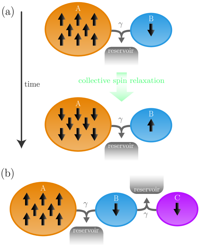
To illustrate how we can extend the model of Fig. 1(a) in Ref. [22, 21], consider the system depicted in Fig. 1(b): In addition to the two spin domains of Fig. 1(a) we add another spin domain collectively coupled with domain to a second reservoir. That is, domains and are collectively coupled to the same zero-temperature reservoir and domains and are collectively coupled to a different zero-temperature reservoir. This means we have the simultaneous action of two collective dissipators, and . For an initial state of
| (4) |
we can expect that for sufficiently large, the coupling to the first reservoir will result in the spins in relaxing to the ground state and the single spin in will move to its excited state. For large , domains and will relax at a time that scales with due to the superradiant decay [40, 41]. We can then consider the coupling to the second reservoir. In this case, the single spin in will be excited (for large ) and the single spin in has already been initialised in its ground state. With the collective coupling to the second reservoir, we can expect these two spins to end in an entangled state. In fact, for , we can expect the relaxation of and to proceed to the steady state described in equation (1) which is an entangled state with entanglement of formation , that is ebits.
In this work we explore the generation of entanglement through multiple spin domains with multiple reservoir couplings. Unlike previous works investigating entangling qubits through interaction with a common reservoir [9, 10, 11, 27, 28, 29, 30, 31, 32], we will show here generation of entanglement between two spins in separate domains which have never interacted and are not even coupled to the same reservoir. In particular, we will also see the amount of entanglement (between qubits not coupled to the same reservoir) to be of similar level to that of the previously mentioned example of two qubits collectively coupled to the same zero temperature reservoir. This paper is arranged in the following way: In Sec. II we present details of the model considered in this work. In Sec. III, we use that model to analyse the capabilities of our system to distribute entanglement. We then look at how entanglement distribution is affected by realistic conditions such as individual decay, dephasing and thermal reservoirs in Sec. IV. Finally, we will also show how multiple system-reservoir couplings can be used to generate tripartite entangled states in Sec. V, before presenting our summary and conclusions in Sec. VI.
II Our model
The system we examine in this work consists of separate spin domains, each consisting of identical spin-1/2 particles with frequency . Although in our system, we assume each spin has the same energy, entanglement can still be generated through a common environment when this is not the case [42]. The spins in two neighbouring spin domains are collectively coupled to a bosonic reservoir. Additionally, our system is symmetric under exchange of two spin-1/2 particles in a given spin domain. The Hamiltonian for our system of spin domains and reservoirs is given by:
| (5) |
where the operators () are the creation (annihilation) operators of the bosonic mode of the reservoirs with frequency . The operators are the collective spin operators for the spin domain and are given by where are the Pauli spin operators with . The collective spin raising and lowering operators for the spin domain are . In (5), the first term represents the Hamiltonian of the spin domains, the second term represents the Hamiltonian of the bosonic reservoirs and the third term represents the interaction between the spin domains and the reservoirs. In the third term, each term in the sum over reservoirs describes the coupling between the and spin domain which are collectively coupled to the bosonic reservoir, with () representing the emission (absorption) amplitudes that fix the spectral density of the reservoirs, . Within the Born-Markov-secular approximation, the master equation in the rotating frame can be written as [43, 44, 20, 45]:
| (6) | ||||
for bosonic reservoirs at zero temperature with . Previous work has experimentally implemented a double spin domain system coupled to a common resonator where each spin domain consisted of nitrogen-vacancy (NV) ensembles in diamonds [46]. Additionally, the work of Ref. [47] implemented a double nuclear spin-domain system coupled to the same bosonic mode. The nuclear spin ensemble size is on the order of which means that the time scale on which collective effects like superradiant decay occur is extremely fast () while the associated individual dephasing and thermalisation times are much slower (on the order of and respectively). In this work, we primarily consider the case of three spin domains coupled to two reservoirs and therefore our master equation is given specifically by:
| (7) |
where we have used the same reservoir coupling constant for all system-reservoir couplings. Further, we can introduce a scaled time to simplify our considerations.
III Entanglement dynamics
In this work, we extend the results of Ref. [22] to more than two spin domains with more than one reservoir coupling. We will show here that entanglement can be generated not just through collective coupling to the same reservoir but also through a chain setup where entanglement will be generated between spins which are not coupled to the same reservoir.
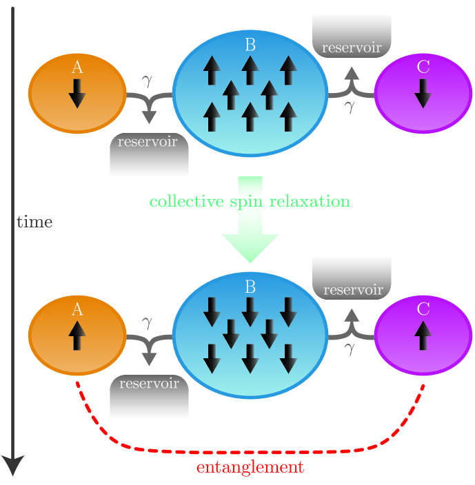
To begin, we will conisder here the situation where domains and consist of a single spin in each domain, while the central domain has spins. This is depicted in Fig. 2. Our goal is to entangle the qubits (in domains and ) which are not coupled to the same reservoir. After this sytem evolves in time according to equation (7), through collective spin relaxation, entanglement is generated between all the spins, however, here we primarily focus on the entanglement between the two single spins in domains and . In the remainder of this paper, we will examine how to maximise the entanglement between spins in and as well as how robust this entanglement is to realistic imperfections.
Our initial state configuration is:
| (8) |
which is depicted in the top part of Fig. 2. However, different initial state configurations can still produce entanglement (see Appendix A). After our initial state (8), evolves in time we then trace out the spins in domain leaving us with the reduced density matrix of the state of the two spins, one in domain and one in domain . To measure the amount of entanglement present in the state , we will use the entanglement of formation, which quantifies the minimum amount of pure state entanglement needed to prepare the state [34]. For an arbitrary state of two qubits, this quantity is given by [36]:
| (9) |
where is given by with . The concurrence is given by where are the square roots of the eigenvalues of the matrix with [35].
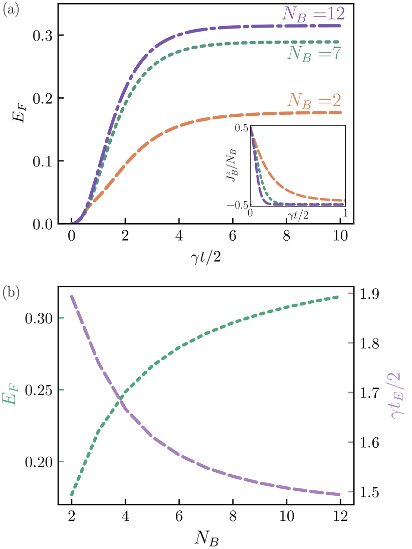
In Fig. 3(a) we plot the entanglement generation dynamics between the two spins in domains and as well as the relaxation dynamics of the initially excited domain . Here we can see that as the number of spins in domain B increases, the decay time decreases. This is indicative of the collective effect of superradiance [40, 41] where the radiation is enhanced and sped up in the presence of mutliple emitters. The increase in spin domain size also contributes to enhanced entanglement dynamics - that is the speed of entanglement generation is increased as is the amount of entanglement present between qubits in and . Note that only collective dissipation into a zero temperatature reservoir is govering the dynamics, and for this case, the entanglement present in the steady state remains and does not decay. We also emphasise here that entanglement is generated between spins which are not coupled to the same reservoir. For the system size of , the entanglement generated between spins in domains and is ebits.
Next in Fig. 3(b), we plot the maximum value of the entanglement of formation (reached at steady state) as well as the value of where is the time for entanglement between and to reach half of the maximum entanglement present during the system evolution. It can clearly be seen that the entanglement distribution is enhanced (more entanglement and faster distribution) for a large spin domain size in . Results here are limited to small total system sizes () due to the memory required to simulate the combined system. As can be seen from Fig 3(b) as we increase , the increase in entanglement is rapid at first, however the growth steadily slows. Thus, for even bigger the payoff with increased entanglement between and will not be significant. We find that for , the steady state of the reduced system goes to
| (10) |
where , and thus the entanglement of formation of this state is the same as the first example in the introduction, that is . In Appendix B, we also illustrate the steady state solution for any spin population with initial state .
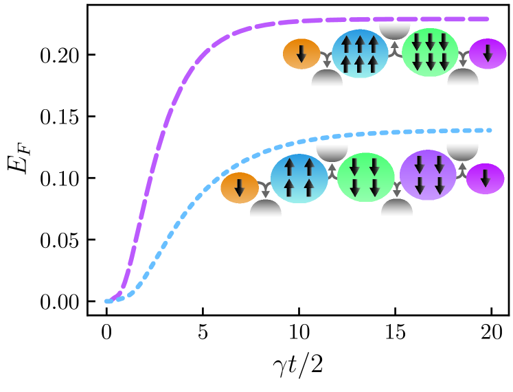
While the previous results focus on distributing entanglement between spins in the outer domains of a three spin domain chain, entanglement generation through collective spin relaxation is not limited to three domains. In Fig. 4 we present results for the entanglement between the single spins in the outer domains of spin domain chains consisting of four (pink, dashed line) and five (blue, dotted line) spin domains. These dynamics use the initial state depicted in the inset diagrams in Fig. 4 respectively, that is all spins initialised in the ground state with the exception of domain which has all spins initialised in the excited state. While we only show entanglement for a single spin domain population configuration for four and five domains, as before, entanglement between outer qubits is maximised for larger spin populations of the middle domains. Here, we have constrained the total number of spins in all middle domains to be the same (12 spins), however the top line uses 12 spins split between two spin-domains and the bottom line uses 12 spins split between three spin-domains. These results are limited due to the total size of the system however, they show that entanglement can be distributed between qubits separated by two or three spin domains which are in turn connected by collective coupling to three or four reservoirs. For this result, as is the case with the previous results, the only effect taken into account in this model is collective decay into zero-temperature reservoirs. In this case, we observe constant entanglement which does not decay in the steady state.
IV Individual decay and dephasing
The results contained in previous section are interesting but represent the highly specific and idealized system of collective relaxation with a zero-temperature bath and with no other individual effects present. It is important to consider more realistic models, which includes effects such as dephasing, individiual spin relaxation and non-zero temperature reservoirs, and examine how these aspects may alter the previously observed entanglement generation.
For the three domain system depicted in Fig. 2, we now incorporate finite temperature reservoirs as well as dephasing and individual relaxation. This yields the following master equation, again in the rotating frame of the system [47]:
| (11) | ||||
In (11), the first and second terms correspond to the collective thermalisation between the pairs of spin domains ( and , and respectively) and the thermal reservoir. Associated with that reservoir is the Bose-Einstein distribution for a given temperature and with Boltzman constant . Next, the third and fourth terms in (11) correspond to individual thermalisation of the spins. Finally, the last term corresponds to dephasing. To summarise, the first line in (11) corresponds to collective effects while the second line corresponds to individual effects associated with thermalization and dephasing. Note that the individual and collective thermalisation occurs with the same system-reservoir coupling constant .
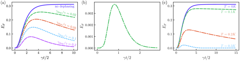
In Fig. 5(a), we plot the entanglement dynamics of the original system with no dephasing (pink, dashed line) as well as the entanglement between spins in domains and with various dephasing rates of (broken lines). We observe a reduction in peak entanglement generated through the system-bath evolution in time but also a gradual reduction in the entanglement present in the steady state. For the results in Fig. 5(a), the dephasing is the only additional effect present, the reservoirs remain at zero temeperature () and there is no individual decay.
We then examine the entanglement generation capabilities of our system under the effects of individual spin coupling to the reservoir. In this case, the spins all have individual as well as the collective dissipation. Again, we shall keep the bosonic reservoir to zero temperature to isolate the effect of individual decay on entanglement dynamics. We find that individual coupling has a signficant detrimental effect on the entanglement present. Shown in Fig. 5(b) is the entanglement dynamics between single spins in domains and . Note the significantly smaller scale of the y-axis in Fig. 5(b) relative to the other results in this work. The maximum entanglement of formation produced in this case is . Note that as the system size increases (number of spins), the superradiant collective effects occur on a much faster time scale than the individual one and most likely dephasing. For example in NV centers in diamond, the collective relaxation can be of order of microseconds, while the individual one is 10 orders of magnitude larger [48].
Lastly, the temperature of the thermal reservoir also substantially affects the entanglement generated through this system. Shown in Fig. 5(c) is the entanglement dynamics between qubits in and for thermal reservoirs of various temperatures for spin domain population of . For this result, we keep only collective spin-reservoir coupling to the bath. As can be seen in Fig. 5(c), the entanglement generated through our system is highly sensitive to the temperature of the thermal reservoirs. As the temperature increases, less entanglement is generated and in the steady state entanglement is also reduced.
We have seen in this section the impact of realistic effects on entanglement distribution via collective dissipation with multiple spin domains and reservoirs. While it is clear that entanglement can still be generated between spins in domains and , it significantly decreases if individual decay or finite temperatures are taken into account. Further, the constant, non-decaying entanglement in the steady state observed in Sec. III is no longer present once any of these effects are taken into account. In the results of Figs. 5(a)-(c) we observe a decline in the entanglement of formation over time. However, individual process are always detrimental to entanglement between spins, and therefore the decay of the entanglement in the results of Fig. 5 is to be expected.
V Tripartite negativity
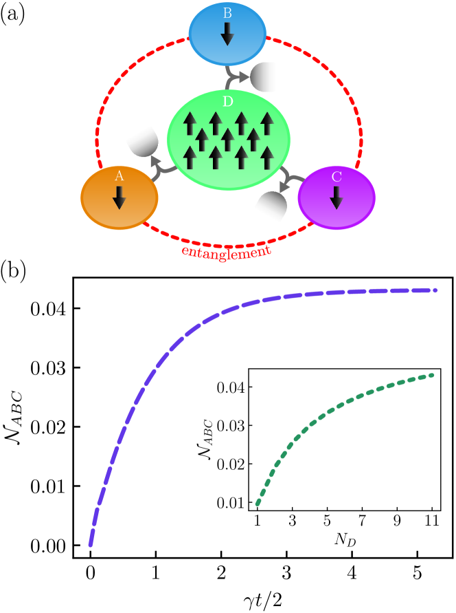
The previous results in this work focused solely on entangling two qubits through collective spin relaxation with multiple collective spin-reservoir couplings. In this section, we will show how this same process can be utilised to generate tripartite entanglement between three spins. Consider the setup shown in Fig. 6(a). This set up is reminiscent of a spin-star configuration [49, 50] but we emphasise again the spins are not directly coupled, merely collectively coupled to the same reservoir as other spins. Here, a central spin-domain (labelled D) contains many spins and is collectively coupled to three bosonic reservoirs with three other spin-domains each containing a single spin only (labelled A, B and C). The system is initialised in the separable state:
| (12) |
Under the process of collective dissipation with the reservoir setup illustrated by the diagram in Fig. 6(a), the steady state of A, B and C (with domain traced out) is given by:
| (13) |
that is, the steady state of the reduced system of three qubits A, B and C is a mixture of the ground state and the W-state which is . Therefore, the steady state of this reduced system has tripartite entanglement between the three remaining qubits. In order to demonstrate the presence of tripartite entanglement in the steady state of this system, we calculate the tripartite negativitity, defined as the geometric mean of the negativities of all bipartitions [51]:
| (14) |
where each of the terms are the bipartite negativities between subsystems and given by with corresponding to the partial transpose of the density matrix with respect to subsystem and is the trace norm of the operator given by [52, 37]. Note that with this definition of the bipartite negativity, maximally entangled Bell states have the negativity of 0.5. Further, for three qubit entangled states, GHZ states yield a tripartite negativity of 0.5 but W states have a tripartite negativity of 0.47. In Fig. 6(b), we give the tripartite negativity generated via the configuration shown in Fig. 6(a) with reservoirs at zero-temperature and no individual effects. The dynamics show clear presence of tripartite negativity in the steady state. For the given spin-domain population of , the steady state tripartite negativity is . Additionally, the inset shows the steady state tripartite entanglement for various values of , the population of the central domain. As the spin-domain population of grows, the steady state contribution of the W-state term [ in (13)] grows larger, and thus the tripartite negativity is maximised for large . However, while this increase is rapid at first, it slows as continues to increase indicating less payoff in tripartite correlations for further increasing the size of the central domain . Nevertheless, the results here show the generation of tripartite correlations between three qubits not coupled to each other or even the same reservoir.
VI Summary and conclusions
We have shown here how, by utilising reservoir engineering, and with a completely separable initial state, entanglement can be generated between two spins which are not coupled to each other or even coupled to the same reservoir. We have focused mostly here on the case where the two spins collectively decay into different reservoirs with a single common spin domain collectively decaying into both reservoirs. For this case, the entanglement is maximised for a large number of spins in the central domain. The speed of entanglement generation is also maximised for a larger spin population in the central domain. Additionally, the entanglement betweeen the qubits not coupled to the same reservoir, can approach the level of entanglement generated when two qubits are collectively coupled to the same zero-temperature reservoir. Entanglement generation via this mechanism is not limited to the three spin-domain case, but can also occur between qubits in the outer domains of four and five domain systems as well as entangling three qubits using a large central domain of many spins.
The results in Sec. IV show that, as expected, when realistic effects are taken into account the entanglement generation between spins suffers significantly. With dephasing or individual spin-reservoir coupling, not only is the maximum entanglement generated reduced, the entanglement in the steady state also decays over time. However, we emphasise that for large enough ensemble size, the collective effects will occur on a timescale that is much faster than that of the individual effects. Additionally, finite temperature reservoirs also reduce the maximum entanglement and cause the steady state entanglement to decay. While the results here predict rather small entanglement generation, further optimisation may significantly increase the maxium entanglement of qubits and make it more robust against imperfections.
VII Acknowledgements
C. W. W. acknowledges financial support by the Deutsche Forschungsgemeinschraft (DFG, German Research Foundation) – Project No. 496502542 (WA 5170/1-1). This work was supported by the JSPS KAKENHI Grants 19H00662 & 21H04880, the MEXT Quantum Leap Flagship Program (MEXT QLEAP) Grant JPMXS0118069605 and the Moonshot R&D Program Grant JPMJMS226C. We are grateful for the help and support provided by the Scientific Computing and Data Analysis section of the Research Support Division at OIST.
Appendix A Alternate initial states
In Sec. III, we showed the dynamics of entanglement generation in our three spin-domain system with the initial state where the middle and most populated spin domain is initialised with all spins in the excited state. This state can also be written in the notation . However, this is not the only configuration that can produce entanglement through collective spin relaxation. In the following, we will explore other initial states and their effect on the steady state entanglement produced via this mechanism.
As we consider the collective coupling of many spins to the same reservoir, a necessary condition of the collective coupling is that the spins are indistinguishable from the perspective of the reservoir. Thus we limit ourselves to initial conditions that are permutationally symmetric within each spin ensemble. These states of permutational symmetry are the so-called Dicke states, and apart from the lowest and highest energy Dicke states (ground or fully excited states respectively), the Dicke states have significant entanglement [53, 54]. In this work, our goal is to start with an initially separable state, and via reservoir engineering, result in the system in a highly entangled steady state. Thus, in exploring alternate initial states, we will limit ourselves to only the separable permutationally symmetric states, which are the fully excited state or ground state of each spin ensemble.
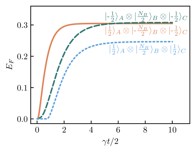
In considering a three spin-ensemble system, this leaves us with two possible initial states for each of the three spin-ensembles, thus leaving eight possible configurations. We will briefly go over the outcomes for each of the eight configurations here. Firstly, with the initial state as the ground state of the entire system, , this trivially produces no dynamics as it does not decay and thus remains in the fully separable ground state. In Fig. 7, we have plotted the entanglement dynamics for three different intitial states. Again, this is the entanglement of formation between the single spins in domains and after the spins in have been traced out. The dark green, dashed line shows the entanglement for the case studied in the main text of this paper, where domains and , of spin populations , are initialised in the ground state and the central domain, of spin population , is initialised in the excited state. This is indicated by the line labelled on Fig. 7. On this plot, we also show the entanglement dynamics for the inital condition which is given by the solid orange line. This solid orange line also represents the entanglement dynamics of the equivalent initial condition of . Thus, three different initial conditions all produce strikingly similar entanglement levels in the steady state.
The strong entanglement in the steady state reached from the initial condition (blue, dotted line in Fig. 7) highlights the novelty of the system considered in this work. To explain this, consider the following: If the three spin ensembles , and were all coupled to a single reservoir, under the collective dissipator , the system would relax to the fully separable ground state of the entire system. As can be seen on Fig. 7, the steady state from this initial condition is highly entangled. This means that, as the system relaxes, a significant proportion of the state remains in an entangled dark state and this is purely due to the collective coupling to two zero-temperature reservoirs, that is the simultaneous action of the dissipators and .
The remaining initial conditions of and with its equivalent produce very little entanglement in the steady state. All three initial states have less than ebits of entanglement of formation. Thus, we can say that, for three spin ensembles, of the eight possible initial state configurations, four of these configurations produce significant steady state entaglement.
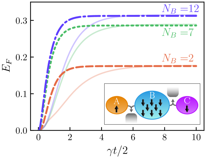
In Fig. 8, we take a closer look at the entanglement dynamics for the initial state
| (1) |
and use this initial state to reproduce the result of Fig. 3(a). As was already observed in Fig. 7, the maximum entanglement generated from intial state (1) is remarkably similar albeit slightly lower than that generated from initial state (8). This can be seen in Fig. 8 by comparing the dotted, dashed and dash-dotted lines with their corresponding solid, transparent line of the same color. The system reaches the maximum entanglement slightly faster for initial condition (1) than (8). Additionally, we find again here, an enhancement in entanglement dynamics, that is faster and more entanglement in the steady state for a larger number of spins . However, it is worth emphasising that the number of excitations in the initial state for all lines in Fig. 8 is fixed at 1. This indicates that it is not the collective, superradiant decay of many spins that enhances the entanglement dynamics, but simply the presence of many spins interacting collectively with the same reservoirs.
Finally, we ask what is the effect of mixed initial state preparation on the steady state entanglement produced in this scheme. As all other results in this work use pure initial states, it is wothwhile to examine whether imperfect state preparation can be detrimental to the steady state entanglement. To answer this question, we return to the main initial condition examined in this work and consider the case where the preparation of the central domain is imperfect and a mixed state is prepared instead. We can model this by the following state
| (2) |
that is, a mixture of the target state and the maximally mixed state, given by the identity matrix . We assume that preparation of the ground state can be done with high fidelity, thus the intial state of the total system is given by:
| (3) |
with defined as in (2). In Fig. 9, we give the steady state entanglement of formation between the single spins in and for a given initial state fidelity . To be precise, is the fidelity of the initial state with the target state , that is . On Fig. 9, we can see that while a decrease in initial state fidelity does have a detrimental impact on the steady state entanglement, the scheme still produces significant entanglement even when the initial state is not completely pure.
Appendix B Steady state and entanglement behavoir for
In this section, we illustrate how the steady state of our system for any (population of the central spin domain) can be found for the specific given initial condition (1). To begin, we acknowledge that through numerical simulation we have found that for a system initialised in the state:
| (4) |
the steady state reached under collective spin relaxation according to master equation (7) is given by:
| (5) |
the first term is the ground state of the total system and the second term is a dark state that does not decay under either dissipator or . While such a dark state is not unique, for our initial state, the form of this particular dark state is always:
| (6) |
where is needed for normalisation and is given by
| (7) |
We stress that all numerical simulations (which have been performed for ) have yielded the steady state as (5) with the given dark state (6). Thus, while we know the dark state for any , to fully characterise the steady state we still need to find the dependence of on , that is the proportion of the state that remains entangled and in the dark state as the system relaxes to its steady state.
To find this dependence of on we start by examining a simple case of , and . This system is initialised in the state
| (8) |
and will relax to a steady state of the form
| (9) |
where for , this dark state is:
| (10) |
We now define two new states, and, as the initial state (1) only contains a single excitation, we only need to be concerned with the single excitation subspace of the total system. For convenience, we choose the two states to be the following:
| (11) |
These states were chosen as it can be easily verified that a system starting in initial state or and evolving under the master equation (7), will relax to the ground state of the total system . Note that the states , and are all mutually orthogonal and if we wanted to define a basis to span the entire single excitation subspace, the remaining basis state would be which is also a dark state under both dissipators or . However, we only need , and as the initial state (8) can be written in terms of these states:
| (12) |
In a similar fasion as the example in the introduction, we can now write down the form of the steady state because we know that the first two terms in (12) will relax to the ground state while the last term is a dark state and does not decay. Thus, the steady state of the total system is:
| (13) |
Therefore, for , we have .
We are interested in the entanglement between spins in and and from (13), we can trace out the two middle spins belonging to domain and be left with the reduced denisty matrix of the spins in and . This is given by:
| (14) |
with . In fact, the form of the reduced density matrix for this problem is always:
| (15) |
While the parameter in (5) describes the proportion of the state that remains in the dark state, the parameter in (15) describes the proportion of the reduced state that is in the entangled Bell state, specifically, the triplet state. As shown above, for , . This analysis can be repeated for with the crucial step being defining the dark state (6) and the two other states and and then using such states to express the initial state. While the formula for the dark state is given in (6), the states and can be generalised for higher spin populations in a straightforward way. For , we have
| (16) |
while for we have:
| (17) |
With such definitions, one needs to express the initial state in terms of , and and from this we know that the dark state component does not decay while the and components decay fully to the ground state. Thus we can find the proportion of the state that remains in the dark state, and subsequently identify the dependence of on . We shall summarise the findings here: The steady state of the total system is given by (5), with the dark state defined as in (6), and with
| (18) |
For the reduced system of two single spins in domains and , the steady state is defined as in (15) with
| (19) |
To quantify the entanglement of the two qubit reduced state, we again use the concurrence, which for this state (15) is simply: and thus the concurrence of the two qubit state for a given is
| (20) |
and the entanglement of formation can be calculated via:
| (21) |
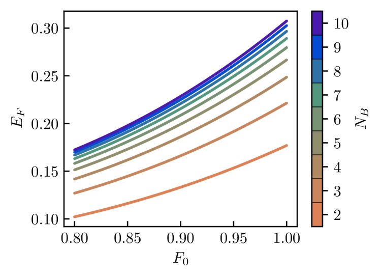
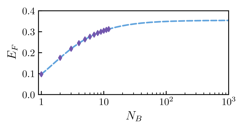
In Fig. 10, we show the behavoir of the entanglement of formation for the range of . As the system size increases, so too does the proportion of the state that remains in the Bell state. For , this value goes to . This means that the steady state of the two qubits in this limit is given by
| (22) |
and the entanglement of formation for this state is
| (23) |
References
- Vidal [2003] G. Vidal, Efficient Classical Simulation of Slightly Entangled Quantum Computations, Physical Review Letters 91, 147902 (2003).
- Ekert and Jozsa [1998] A. Ekert and R. Jozsa, Quantum algorithms: entanglement–enhanced information processing, Philosophical Transactions of the Royal Society of London. Series A: Mathematical, Physical and Engineering Sciences 356, 1769 (1998).
- Gottesman and Chuang [1999] D. Gottesman and I. L. Chuang, Demonstrating the viability of universal quantum computation using teleportation and single-qubit operations, Nature 402, 390 (1999).
- Raussendorf and Briegel [2001] R. Raussendorf and H. J. Briegel, A One-Way Quantum Computer, Physical Review Letters 86, 5188 (2001).
- Gisin and Thew [2007] N. Gisin and R. Thew, Quantum communication, Nature Photonics 1, 165 (2007).
- Jozsa and Linden [2003] R. Jozsa and N. Linden, On the role of entanglement in quantum-computational speed-up, Proceedings of the Royal Society of London. Series A: Mathematical, Physical and Engineering Sciences 459, 2011 (2003).
- Życzkowski et al. [2001] K. Życzkowski, P. Horodecki, M. Horodecki, and R. Horodecki, Dynamics of quantum entanglement, Physical Review A 65, 012101 (2001).
- Rajagopal and Rendell [2001] A. K. Rajagopal and R. W. Rendell, Decoherence, correlation, and entanglement in a pair of coupled quantum dissipative oscillators, Physical Review A 63, 022116 (2001).
- Hor-Meyll et al. [2009] M. Hor-Meyll, A. Auyuanet, C. V. S. Borges, A. Aragão, J. A. O. Huguenin, A. Z. Khoury, and L. Davidovich, Environment-induced entanglement with a single photon, Phys Rev A 80, 042327 (2009).
- Braun [2002] D. Braun, Creation of Entanglement by Interaction with a Common Heat Bath, Physical Review Letters 89, 277901 (2002).
- Kim et al. [2002] M. S. Kim, J. Lee, D. Ahn, and P. L. Knight, Entanglement induced by a single-mode heat environment, Physical Review A 65, 040101 (2002).
- Schneider and Milburn [2002] S. Schneider and G. J. Milburn, Entanglement in the steady state of a collective-angular-momentum (Dicke) model, Physical Review A 65, 042107 (2002).
- Verstraete et al. [2009] F. Verstraete, M. M. Wolf, and J. Ignacio Cirac, Quantum computation and quantum-state engineering driven by dissipation, Nature Physics 5, 633 (2009).
- Keck et al. [2018] M. Keck, D. Rossini, and R. Fazio, Persistent currents by reservoir engineering, Phys. Rev. A 98, 053812 (2018).
- Damanet et al. [2019] F. m. c. Damanet, E. Mascarenhas, D. Pekker, and A. J. Daley, Controlling quantum transport via dissipation engineering, Phys. Rev. Lett. 123, 180402 (2019).
- Yanay and Clerk [2018] Y. Yanay and A. A. Clerk, Reservoir engineering of bosonic lattices using chiral symmetry and localized dissipation, Physical Review A 98, 043615 (2018).
- Kurizki et al. [2015] G. Kurizki, P. Bertet, Y. Kubo, K. Mølmer, D. Petrosyan, P. Rabl, and J. Schmiedmayer, Quantum technologies with hybrid systems, Proceedings of the National Academy of Sciences 112, 3866 (2015).
- Wallquist et al. [2009] M. Wallquist, K. Hammerer, P. Rabl, M. Lukin, and P. Zoller, Hybrid quantum devices and quantum engineering, Physica Scripta 2009, 014001 (2009).
- Xiang et al. [2013] Z.-L. Xiang, S. Ashhab, J. Q. You, and F. Nori, Hybrid quantum circuits: Superconducting circuits interacting with other quantum systems, Reviews of Modern Physics 85, 623 (2013).
- Breuer and Petruccione [2002] H. P. Breuer and F. Petruccione, The Theory of Open Quantum Systems (Oxford University Press, Oxford, 2002).
- Hama et al. [2018a] Y. Hama, W. J. Munro, and K. Nemoto, Relaxation to Negative Temperatures in Double Domain Systems, Physical Review Letters 120, 060403 (2018a).
- Hama et al. [2018b] Y. Hama, E. Yukawa, W. J. Munro, and K. Nemoto, Negative-temperature-state relaxation and reservoir-assisted quantum entanglement in double-spin-domain systems, Physical Review A 98, 052133 (2018b).
- Stegmann et al. [2020] P. Stegmann, J. König, and B. Sothmann, Relaxation dynamics in double-spin systems, Physical Review B 101, 075411 (2020).
- Quach and Munro [2020] J. Q. Quach and W. J. Munro, Using Dark States to Charge and Stabilize Open Quantum Batteries, Phys. Rev. Appl. 14, 024092 (2020).
- Dias et al. [2021] J. Dias, C. W. Wächtler, V. M. Bastidas, K. Nemoto, and W. J. Munro, Reservoir-assisted energy migration through multiple spin domains, Physical Review B 104, L140303 (2021).
- Aolita et al. [2015] L. Aolita, F. d. Melo, and L. Davidovich, Open-system dynamics of entanglement:a key issues review, Reports on Progress in Physics 78, 042001 (2015).
- Oh and Kim [2006] S. Oh and J. Kim, Entanglement between qubits induced by a common environment with a gap, Physical Review A 73, 062306 (2006).
- Contreras-Pulido and Aguado [2008] L. D. Contreras-Pulido and R. Aguado, Entanglement between charge qubits induced by a common dissipative environment, Physical Review B 77, 155420 (2008).
- Maniscalco et al. [2008] S. Maniscalco, F. Francica, R. L. Zaffino, N. Lo Gullo, and F. Plastina, Protecting Entanglement via the Quantum Zeno Effect, Physical Review Letters 100, 090503 (2008).
- Francica et al. [2009] F. Francica, S. Maniscalco, J. Piilo, F. Plastina, and K.-A. Suominen, Off-resonant entanglement generation in a lossy cavity, Physical Review A 79, 032310 (2009).
- Lin et al. [2013] Y. Lin, J. P. Gaebler, F. Reiter, T. R. Tan, R. Bowler, A. S. Sørensen, D. Leibfried, and D. J. Wineland, Dissipative production of a maximally entangled steady state of two quantum bits, Nature 504, 415 (2013).
- Shankar et al. [2013] S. Shankar, M. Hatridge, Z. Leghtas, K. M. Sliwa, A. Narla, U. Vool, S. M. Girvin, L. Frunzio, M. Mirrahimi, and M. H. Devoret, Autonomously stabilized entanglement between two superconducting quantum bits, Nature 504, 419 (2013).
- Benatti and Floreanini [2006] F. Benatti and R. Floreanini, Entangling oscillators through environment noise, Journal of Physics A: Mathematical and General 39, 2689 (2006).
- Bennett et al. [1996] C. H. Bennett, G. Brassard, S. Popescu, B. Schumacher, J. A. Smolin, and W. K. Wootters, Purification of noisy entanglement and faithful teleportation via noisy channels, Phys. Rev. Lett. 76, 722 (1996).
- Wootters [1998] W. K. Wootters, Entanglement of Formation of an Arbitrary State of Two Qubits, Physical Review Letters 80, 2245 (1998).
- Hill and Wootters [1997] S. A. Hill and W. K. Wootters, Entanglement of a Pair of Quantum Bits, Physical Review Letters 78, 5022 (1997).
- Vidal and Werner [2002] G. Vidal and R. F. Werner, Computable measure of entanglement, Physical Review A 65, 032314 (2002).
- Plenio [2005] M. B. Plenio, Logarithmic Negativity: A Full Entanglement Monotone That is not Convex, Physical Review Letters 95, 090503 (2005).
- Munro et al. [2021] W. J. Munro, J. Dias, and K. Nemoto, Collective effects in hybrid quantum systems, in Hybrid Quantum Systems, edited by Y. Hirayama, K. Ishibashi, and K. Nemoto (Springer Nature Singapore, Singapore, 2021) pp. 43–60.
- Dicke [1954] R. H. Dicke, Coherence in spontaneous radiation processes, Phys. Rev. 93, 99 (1954).
- Gross and Haroche [1982] M. Gross and S. Haroche, Superradiance: An essay on the theory of collective spontaneous emission, Physics Reports 93, 301 (1982).
- Auyuanet and Davidovich [2010] A. Auyuanet and L. Davidovich, Quantum correlations as precursors of entanglement, Physical Review A 82, 032112 (2010).
- Gorini et al. [2008] V. Gorini, A. Kossakowski, and E. C. G. Sudarshan, Completely positive dynamical semigroups of N‐level systems, Journal of Mathematical Physics 17, 821 (2008).
- Lindblad [1976] G. Lindblad, On the generators of quantum dynamical semigroups, Communications in Mathematical Physics 48, 119 (1976).
- Carmichael [2013] H. J. Carmichael, Statistical methods in quantum optics 1: master equations and Fokker-Planck equations (Springer Science & Business Media, 2013).
- Astner et al. [2017] T. Astner, S. Nevlacsil, N. Peterschofsky, A. Angerer, S. Rotter, S. Putz, J. Schmiedmayer, and J. Majer, Coherent Coupling of Remote Spin Ensembles via a Cavity Bus, Physical Review Letters 118, 140502 (2017).
- Fauzi et al. [2021] M. H. Fauzi, W. J. Munro, K. Nemoto, and Y. Hirayama, Double nuclear spin relaxation in hybrid quantum Hall systems, Physical Review B 104, L121402 (2021).
- Angerer et al. [2018] A. Angerer, K. Streltsov, T. Astner, S. Putz, H. Sumiya, S. Onoda, J. Isoya, W. J. Munro, K. Nemoto, J. Schmiedmayer, and J. Majer, Superradiant emission from colour centres in diamond, Nature Physics 14, 1168 (2018).
- Anzà et al. [2010] F. Anzà, B. Militello, and A. Messina, Tripartite thermal correlations in an inhomogeneous spin–star system, Journal of Physics B: Atomic, Molecular and Optical Physics 43, 205501 (2010).
- Hutton and Bose [2004] A. Hutton and S. Bose, Mediated entanglement and correlations in a star network of interacting spins, Physical Review A 69, 042312 (2004).
- Sabín and García-Alcaine [2008] C. Sabín and G. García-Alcaine, A classification of entanglement in three-qubit systems, The European Physical Journal D 48, 435 (2008).
- Życzkowski et al. [1998] K. Życzkowski, P. Horodecki, A. Sanpera, and M. Lewenstein, Volume of the set of separable states, Phys. Rev. A 58, 883 (1998).
- Garraway [2011] B. M. Garraway, The dicke model in quantum optics: Dicke model revisited, Philosophical Transactions of the Royal Society A: Mathematical, Physical and Engineering Sciences 369, 1137 (2011).
- Agarwal [2013] G. Agarwal, Quantum Optics, Quantum Optics (Cambridge University Press, 2013).