Entanglement harvesting in the presence of a reflecting boundary
Abstract
We study, in the framework of the entanglement harvesting protocol, the entanglement harvesting of both a pair of inertial and uniformly accelerated detectors locally interacting with vacuum massless scalar fields subjected to a perfectly reflecting plane boundary. We find that the presence of the boundary generally degrades the harvested entanglement when two detectors are very close to the boundary. However, when the distance between detectors and the boundary becomes comparable to the interaction duration parameter, the amount of the harvested entanglement approaches a peak, which even goes beyond that without a boundary. Remarkably, the parameter space of the detectors’ separation and the magnitude of acceleration that allows entanglement harvesting to occur is enlarged due to the presence of the boundary. In this sense, the boundary plays a double-edged role on entanglement harvesting, degrading in general the harvested entanglement while enlarging the entanglement harvesting-achievable parameter space. A comparison of three different acceleration scenarios of the detectors with respect to the boundary, i.e., parallel, anti-parallel and mutually perpendicular acceleration, shows that the phenomenon of entanglement harvesting crucially depends on the acceleration, the separation between two detectors and the detectors’ distance from the boundary.
I Introduction
Quantum entanglement has been considered as a crucial physical resource in quantum information science such as quantum communication RC ; Bh , quantum teleportation Bg , quantum cryptography Ea and dense coding Bh , etc, and it has been extensively studied in various physical aspects. Recently, a lot of interest has been attracted in the role played by entanglement in a variety of physical contexts, such as the critical phenomena in condensed matter systems Osterloh:2002 ; Vidal:2003 ; Amico:2008 , the description of non-classical states of light LM:1995 ; Weedbrook:2012 , the explanation for the origin of black hole entropy Bombelli:1986 ; Calla:1994 ; Srednicki:1993 and the anti-de Sitter/conformal field theory correspondence Ryu:2006 .
It has been realized that vacuum can be a resource of entanglement for the vacuum state of a free quantum field can maximally violate Bell’s inequalities as was shown in the formal algebraic quantum field theory Summers:1985 ; Reznik:2005 , and a pair of initially uncorrelated detectors can extract entanglement from vacuum via locally interacting with vacuum fields VAN:1991 ; Reznik:2003 . This phenomenon of entanglement extraction has been extensively studied in an operational approach employing the Unruh-DeWitt (UDW) detector model Steeg:2009 ; Olson:2011 ; BLHu:2012 ; EDU:2012-2 ; Martin-Martinez:2014gra ; EDU:2013 ; Nambu:2013 ; Pozas-Kerstjens:2015 ; EDU:2016-1 ; EDU:2016-2 ; Zhjl:2018 ; Zhjl:2019 ; Ng:2018 ; Ng:2018-2 ; Zhjl:2020 , which is now known as the entanglement harvesting protocol Salton-Man:2015 . A lot of studies have demonstrated that the phenomenon of entanglement harvesting involves a combination of relativistic and quantum effects, and it is sensitive to the spacetime topology Steeg:2009 ; EDU:2016-1 ; Zhjl:2018 ; Zhjl:2019 ; Ng:2018-2 , intricate motions of detectors Zhjl:2020 , and even cosmology EDU:2012-2 ; Martin-Martinez:2014gra . More recently, the entanglement harvesting in some special circumstances has been investigated, such as in the background with black holes Zhjl:2018 , in the presence of gravitational waves XQ:2020 and near the horizon mimicked by imposing a moving mirror as the boundary CW:2019 ; CW:2020 . In particular, the entanglement harvesting has been studied for inertial detectors in 1+1 dimensional moving mirror spacetimes in Ref. CW:2019 , where it was argued that there exists an entanglement inhibition phenomenon similar to that found for black holes and the concrete harvesting process is sensitive to the mirror trajectory. While, for an accelerated mirror moving along a particular trajectory parameterized by the product-log function, the mimicked effects of horizon on entanglement harvesting have been discussed in Ref. CW:2020 , which reveals a sensitivity of the entanglement harvested to the dynamics of the trajectories and an insensitivity of entanglement to the sign of radiation flux emitted by such an accelerated mirror.
In this paper, we plan to investigate the entanglement harvesting for two UDW detectors at rest or uniformly accelerated near a static perfectly reflecting boundary rather than a drifting mirror that is used to mimic a dynamical spacetime. This would allow us to consider how the reflecting boundary and the motion status of detectors affect the entanglement harvesting phenomenon in a more realistic 1+3 dimensional spacetime. The phenomenon of entanglement harvesting in the circumstance with accelerated detectors necessarily involves both the relativistic effects due to the non-inertial motion of the detectors and quantum effects arising from the modification of quantum vacuum fluctuations of the scalar fields by the presence of a boundary which the detectors are coupled to. Let us note here that the most fascinating effect associated with the uniform acceleration is the Unruh effect, which attests that accelerated detectors in vacuum will observe a thermal radiation spectrum of particles. The thermal noise due to the Unruh effect is generally expected to drive the accelerated detectors to decohere. Therefore, the behavior of entanglement harvesting therein would be an interesting topic, since it is expected to be affected by both the presence of the boundary and the accelerated motion of the detectors which is connected the Unruh effect. Indeed, on one hand, a lot of studies have revealed the influence of acceleration on quantum entanglement via various detector models, including two-level detectors or UDW models Reznik:2003 ; Salton-Man:2015 , harmonic oscillators BLH:2008 ; BLH:2010 , and wave packets Ahmadi:2016 ; Crochowski:2019 . In particular, it was argued in Ref. Salton-Man:2015 that the entanglement extraction can be enhanced for two UDW detectors in anti-parallel acceleration in comparison with those in inertial motion or parallel acceleration. On the other hand, it has been demonstrated that the presence of boundaries in flat spacetime, which changes the spacetime topology and causes modification of fluctuations of quantum fields Birrell:1984 , brings new features to novel quantum effects associated acceleration, such as the Casimir-Polder interaction Rizzuto:2007 ; Passante:2007 ; Zhu:2010 , the modified radiative properties of accelerated atoms Yu:2005ad ; Yu:2006kp ; Rizzuto:2009 , the geometric phase Zhjl:2016 and the modified entanglement dynamics Zhjl:2007 ; Cheng:2018 .
Therefore, questions arise naturally as to what role the boundary would play in performing the entanglement harvesting protocols via a pair of inertial as well as uniformly accelerated detectors and what would happen to the entanglement harvesting for two detectors in different acceleration scenarios near the boundary. To address these questions, we will first consider a pair of inertial detectors and then a pair of uniformly accelerated UDW detectors, which are initially prepared in a separable state and locally interact with the vacuum massless scalar fields near a perfectly reflecting plane boundary. For the case of accelerated detectors, three distinct acceleration scenarios, i.e, parallel acceleration and anti-parallel acceleration with respect to the boundary as well as mutually perpendicular acceleration in a plane parallel to the boundary, will be examined. According to the entanglement harvesting protocol, the reduced density of two detectors can be written in an -type form, and the concurrence as a measure of entanglement, which is employed to characterize the amount of the entanglement harvested from vacuum by such detectors, can be calculated for a chosen switching function.
The paper is organized as follows. In the next section, basic formulae for the UDW detectors locally interacting with vacuum scalar fields are reviewed. In Sec.III, we mainly study the influence of a boundary on the transition probabilities of uniformly accelerated detectors interacting with the quantum fields in a finite duration. In Sec. IV, we consider the entanglement harvesting for both two inertial detectors and two detectors moving along different acceleration trajectories near the boundary, including those of parallel acceleration, anti-parallel acceleration and acceleration in mutually perpendicular directions in a plane parallel to the boundary. The influence of the boundary on the behavior of the entanglement harvesting is examined in detail, with a cross-comparison of the results obtained. Finally, we end up with conclusions in Sec.V.
Throughout this paper we adopt the natural units in which for convenience.
II The basic formulas
Without loss of generality, the two-level point-like detector is treated as the UDW module with a ground state and excited state , which locally interacts with the massless scalar field . Here, denotes the coordinates of spacetime with the subscript specifying which UDW detector we are considering. Let us suppose that the classical spacetime trajectory of the detector is parameterized by its proper time . Then the interaction Hamiltonian for such a detector in the interaction picture takes the following form
| (1) |
where is the coupling strength, is the energy gap of the detector, and denote the ladder operators of the SU(2) algebra, and is the Gaussian switching function which controls the duration of interaction via parameter .
Before the interaction begins, we assume that two UDW detectors (labeled and ) are in their ground state and the field in a vacuum state . Then the joint state of the detectors and the field can be written as . According to the detector-field interaction Hamiltonian (1), the finial state of the system (two detectors plus the field) is given by
| (2) |
where denotes the time ordering operator. For simplicity, the two detectors are assumed to be completely identical with a fixed but not too large energy gap, i.e., and , in the following discussions. Based on the perturbation theory, the density matrix for the finial state of the two detectors can be obtained from Eq. (2) by tracing out the field degrees of freedom, and after some algebraic manipulations, it takes the following form in the basis EDU:2016-1 ; Zhjl:2018 ; Zhjl:2019
| (3) |
where the transition probability reads
| (4) |
and quantities and which characterize nonlocal correlations are given by
| (5) |
| (6) |
where is the Wightman function of the field and represents the Heaviside theta function. Note that the detector’s coordinate time is a function of its proper time, i.e., and , in the above equations.
According to the entanglement harvesting protocol, we can employ the concurrence as a measure of entanglement WW , which specifically quantifies the entanglement harvested by the detectors via local interaction with the fields. For an -type density matrix (II), the concurrence takes a simple form EDU:2016-1 ; Zhjl:2018 ; Zhjl:2019
| (7) |
The concurrence is dependent only on the nonlocal correlation X and the transition probabilities. As a result, the Wightman function of the scalar fields plays a crucial role in entanglement harvesting. In what follows, We will examine the entanglement harvesting phenomenon for both a pair of inertial and uniformly accelerated detectors near a perfectly reflecting plane boundary, focusing on the influence of the presence of the boundary.
III The transition probabilities of detectors near the reflecting boundary
Let us first analyze the transition probabilities. To facilitate the discussion, we assume that a plane boundary is located at , and the uniformly accelerated UDW detector is moving along the trajectories with a distance away from the boundary, that is
| (8) |
where is the proper acceleration and is the detector’s proper time. The Wightman function for vacuum massless scalar fields in four dimensional Minkowski spacetime in the presence of a reflecting boundary is, according to the method of images, given by Birrell:1984
| (9) |
Substituting trajectory (8) and Eq. (III) into Eq. (4), we have, after some manipulations (see Appendix)
| (10) |
where , and with the error function .
An analytical result of Eq. (III) can hardly be found. Fortunately, numerical evaluations can be implemented for a finite duration of interaction ( finite nonzero ). It is worth noting that the second and fourth term in Eq. (III) arise from the image part of the Wightman function, which are dependent on the distance between the boundary and the detector , while the remaining two terms are just those of the transition probabilities of uniformly accelerated detectors in free Minkowski spacetime Zhjl:2020 . In the limit of , the transition probabilities become
| (11) |
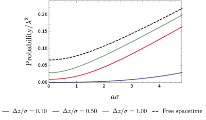
We show our numerical evaluation of Eq.(III&III) in Fig. (1). As we can see there, the transition probabilities for a finite duration generally increase as the acceleration increases, which is consistent with what we expect that high acceleration causes strong thermalization. However, the thermalization is suppressed by the presence of the boundary. Especially, when the detector is very close to the boundary (), the transition probabilities become very small. At the same time, one can also observe that the transition probabilities seem to be an increasing function of which flatten up when becomes relatively large.
IV Entanglement harvesting near the reflecting boundary
In this section, we will examine the phenomenon of the entanglement harvesting, paying particular attention to the influence of the boundary. We start with a discussion of how the reflecting boundary affects the entanglement harvested by two inertial detectors at rest at a certain fixed distance from the boundary, followed by an analysis of two uniformly accelerated detectors. For convenience of comparing the boundary influence in these two circumstances, the trajectories of two accelerated detectors are assumed to align parallel to the boundary plane with a distance away from it as well. The effects of the boundary on the entanglement harvesting in three different acceleration scenarios, i.e., parallel acceleration, anti-parallel acceleration and mutually perpendicular acceleration, are to be analyzed in detail.
IV.1 Entanglement harvesting for inertial detectors
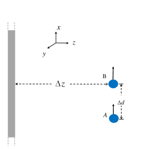
For two detectors at rest which are aligned parallel to the reflecting boundary with a fixed distance from it and separated by a distance , their trajectories can, without loss of generality, be written as
| (12) |
In order to examine the effect of the boundary on the entanglement harvesting for inertial detectors, we should first compute the transition probability given by Eq. (4) and the relevant non-local correlation term given by Eq. (6) along the trajectories (12). The analytical expression of the transition probability of a static detector has already been given by Eq. (III), and particularized here as , can be obtained straightforwardly via the method of Cauchy principle value,
| (13) |
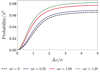
Then the concurrence can be found by substituting Eq. (III) and Eq. (13) into Eq. (7). In order to show the properties of the entanglement harvesting, we plot the concurrence as a function of the distance and the separation in Fig. (2), respectively.
It is worth pointing out that will be vanishingly small when the two detectors are placed infinitely close to the reflecting boundary and so will be the concurrence, suggesting that the entanglement harvesting will be greatly inhibited as is illustrated by Fig. (2a). More interestingly, one may find a peak of the extracted entanglement approximately at the position where is comparable to the interaction duration parameter for a not too large fixed 333If were too large, the extracted entanglement would vanish.. At large enough , the concurrence asymptotically approaches its free space value as expected. Let us note here that these features, e.g., the appearance of peaks of the extracted entanglement, have also been found for inertial detectors in 1+1 dimensional mirror spacetimes in Ref. CW:2019 .
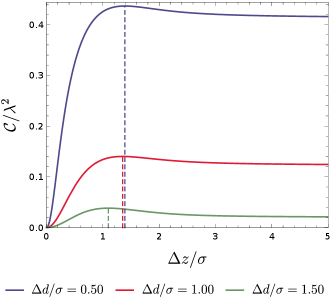
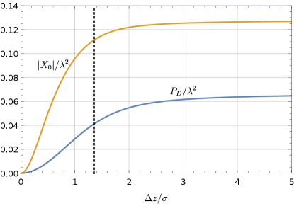
In order to gain an understanding to this property, we show the behaviors of and versus in Fig. (3). As we can see, the reflecting boundary would in general restrain both the transition probabilities and the non-local correlation of the fields . However, as the distance increases to approach , the degree of suppression is different (see the vertical dashed line in Fig. (3)). That is, at the beginning, the difference between and grows as the distance increases. However, when the distance grows across , no longer increases significantly with increasing , while the transition probability still significantly increases for a while. As a result, the difference between and becomes a little smaller, resulting in a peak in the difference therein. As, according to the definition in Eq. (7), the concurrence is in fact a competition between the nonlocal correlation and the transition probabilities, the above analysis explains why the harvested entanglement peaks when the distance is comparable to the parameter . Remarkably, the peak value of the concurrence is even larger than that without a boundary, suggesting that the detectors may harvest more entanglement than when there is no boundary.
Fig. (2b) shows that the concurrence for a fixed distance between detectors and the boundary would rapidly degrade as the detectors’ separation increases. This arises from the fact that is exponentially suppressed as increases (see Eq. (13)), and is consistent with our intuition that the correlation of the detectors would weaken as their inter-separation grows. Once the inter-separation increases beyond a certain value, the concurrence will virtually vanish and entanglement harvesting essentially on longer occurs. So, there exists an entanglement harvesting-achievable range for , which, as shown in the subfigure of Fig. (2b), is sensitive to the distance from the boundary.
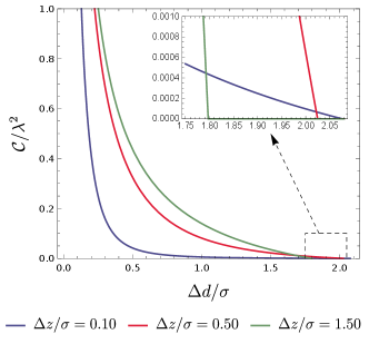
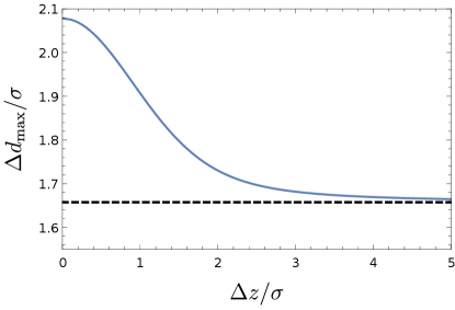
To better understand the influence of the presence of the boundary on the harvesting-achievable range of the separation where entanglement harvesting is possible. Here, we use to stand for the maximum value (or critical value) of the separation , beyond which entanglement harvesting does not occur any more. From Eq. (III) and Eq. (13), we obtain the plot of as a function of (see Fig. (4)). One can see that is obviously a decreasing function of , which means that the presence of the boundary could enlarge the harvesting-achievable range. It should be pointed out here that a on the boundary plane would make no physical sense. This is because the corresponding Wightman function Eq. (III) approaches zero in the limit of , and as a consequence the concurrence then vanishes and does not depend on the parameter .
Now we are in a position to explore the effects of the boundary on the entanglement harvesting of uniformly accelerated detectors. In particular, we will study three acceleration scenarios and make a comparison with the inertial situation.
IV.2 Entanglement harvesting for uniformly accelerated detectors
IV.2.1 Parallel acceleration
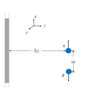
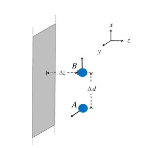
Here, we assume that two detectors are accelerated in parallel with respect to the boundary with the same magnitude of acceleration (see Fig. (5)), the corresponding trajectories satisfy Salton-Man:2015
| (14) |
where represents the separation between two detectors, as measured by an inertial observer at a fixed (i.e., in the laboratory reference frame).
The transition probabilities can be evaluated by using Eq. (III), and the nonlocal correlation term can be obtained by substituting the Wightman function into Eq. (6). Here, we use to denote X in the case of the parallel acceleration where the trajectories of two detectors are described by Eq. (IV.2.1). According to Eq. (6), we have
| (15) |
Letting and , Eq. (15) becomes, after some algebraic manipulations,
| (16) |
where
| (17) |
| (18) |
and
| (19) |
In principle, the transition probabilities of the uniformly accelerated detectors can be calculated by using Eq. (III), and the nonlocal correlation term can also be obtained from Eq. (16). However, analytical results are quite difficult to obtain due to the presence of the Gaussian switching function. So, numerical calculations will be resorted to later on. The concurrence Eq. (7), which quantifies the entanglement harvested by detectors, can be evaluated explicitly, once the values of and transition probabilities are known. Before we show the results of numerical calculations, let us first give the same general analysis for the other two scenarios.
IV.2.2 Anti-parallel acceleration
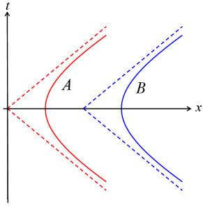
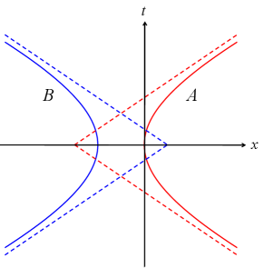
Now, we move on to the case of two detectors with anti-parallel acceleration along -axis (see Fig. (6)). For convenience, we specify the spacetime trajectories of two such detectors in the form as Salton-Man:2015
| (20) |
where denotes the separation between two detectors at the closest approach (i.e., at the origin of the time coordinate), as seen by a rest observer at a constant , namely the closest distance is independent of the acceleration Salton-Man:2015 . It should be point out that the trajectories Eq. (IV.2.2) in general relax the condition of overlapping apexes shared by four Rindler wedges of two detectors.
The transition probabilities can be numerically calculated by using Eq. (III) as well, and the nonlocal correlation term , now represented by , can be obtained by substituting Eq. (IV.2.2) into Eq. (6)
| (21) |
where
| (22) |
Numerically evaluating the transition probability and , we can explore the concurrence to reveal the features of entanglement harvesting, which we will present in detail later.
IV.2.3 The acceleration in perpendicular orientations
In this subsection, we will consider the case of two detectors uniformly accelerated in mutually vertical directions. Concretely, we assume that two detectors are uniformly accelerated in a plane parallel to the boundary, where one detector is accelerated in the -axis and the other accelerated in the -axis (see Fig. (7)).
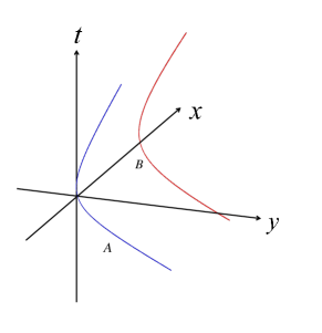
Hence, the spacetime trajectories of the two perpendicularly accelerated detectors take the following form
| (23) |
Similarly, a substitution of Eq. (IV.2.3) into Eq.(6) yields the nonlocal correlation term , denoted by in the present case
| (24) |
where
| (25) |
and
| (26) |
Now with the formulae needed for examining the entanglement harvesting by two detectors uniformly accelerated in all the three different scenarios, we are to show the results of our numerical calculations below.
IV.2.4 The numerical result and cross comparison
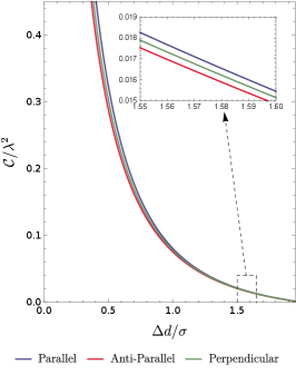
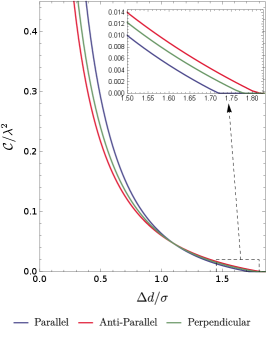
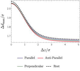
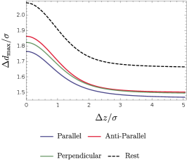
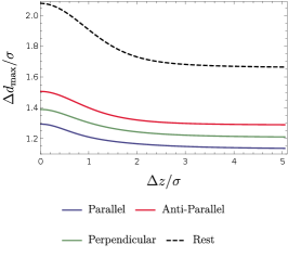
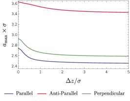
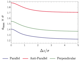
We now turn to explore the entanglement harvesting phenomenon for two detectors in parallel, anti-parallel and mutually perpendicular acceleration via numerical evaluation.We begin by plotting, in Figs. (8) and (9), the concurrence as a function of the distance between the boundary and the detectors, , with other parameters of the system fixed at certain values for all three acceleration scenarios. As we can see, the distance from the boundary significantly influences the harvested entanglement. Particularly, similar to that in the situation of inertial detectors at rest, the entanglement harvesting is greatly inhibited when the detectors are close to the boundary (). It is worth pointing out that the concurrence asymptotically approaches that without a boundary as the distance between the detectors and boundary grows very large (i.e., ), as a result of the fact that the Wightman function reduces to its free-space form in the limit of . In fact, this is valid irrespective of whether the detector is accelerating or not. Again similar to that in the situation of inertial detectors at rest, there also exists, for the same reason, a peak of the extracted entanglement approximately at the position where is comparable to the duration parameter , for both fixed and in all three scenarios. This phenomenon of entanglement enhancement by a boundary was similarly found in Ref. Cheng:2018 where entanglement dynamics of uniformly accelerated polarizable atoms coupled with electromagnetic fields in the presence of a reflecting boundary was examined. Here, the general inhibition of entanglement harvesting and the peak occurrence of the harvested entanglement that arise from the effects of the boundary still remain regardless of whether two detectors are accelerated or not. Interestingly, the location of the peak, as shown in Figs. (8) and (9), is almost independent of the acceleration scenarios, although the magnitude of the peak is noticeably affected by the acceleration scenario. In general, the parallel acceleration case seems to have a comparatively large peak for a small acceleration or separation between two detectors, while for a large acceleration or separation between two detectors the anti-parallel acceleration case takes the place.
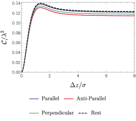
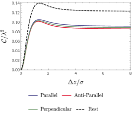
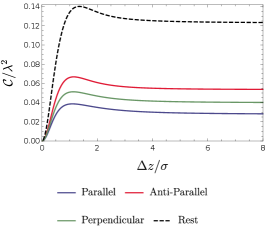
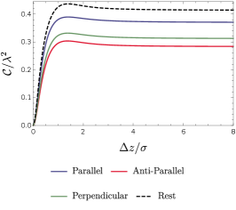
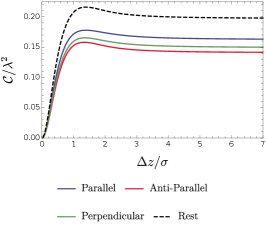
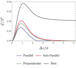
Now let us turn our attention to a cross comparison of the entanglement harvesting in various scenarios. From Fig. (8) and Fig. (9), one can find that the issue of which acceleration scenario is better in terms of entanglement harvesting crucially depends on the value of the acceleration or the detectors’ separation . Since the detectors’ thermalization that arises from the effect of acceleration would generally inhibit the extraction of entanglement, thus the inertial detectors at rest are likely to harvest more entanglement than those in uniform acceleration scenarios at the same distance from the boundary with not too large energy gap . Among three acceleration scenarios, the parallel acceleration case is likely to harvest more entanglement for a small acceleration ( and ). However, in contrast, the anti-parallel acceleration extracts more entanglement for a large acceleration (). Physically, these features can be understood as follows. For a small acceleration, the average detectors’ separation during the interaction with fields characterized by the duration parameter is the dominant factor in the non-local correlation term . The smaller the separation, the large the . As a result, comparatively more entanglement is extracted for the parallel acceleration due to the fact that two detectors in parallel acceleration has a smaller average detectors’ separation (i.e., they spend more time closer to one another). This is consistent with what happens for the inertial detectors. But, for a large acceleration, the decrease of becomes much more complicated as now it is a consequence of the intertwined effects from and , so that the effect of acceleration dominates in the non-local correlation term and overweighs that of the detectors’ separation, resulting in the anti-parallel acceleration scenario harvesting more entanglement although the parallel acceleration case still has a smaller average detectors’ separation.
For a more thorough analysis on the difference in three acceleration scenarios, we plot the concurrence as a function of acceleration with different fixed to compare the influence of acceleration for all three acceleration scenarios in Fig (10), and that of the detectors’ separation with different fixed acceleration to compare the influence of the detectors’ separation in Fig. (11).
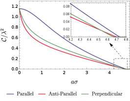
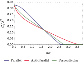
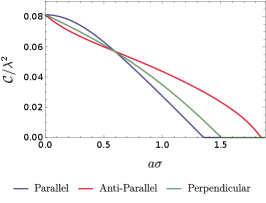
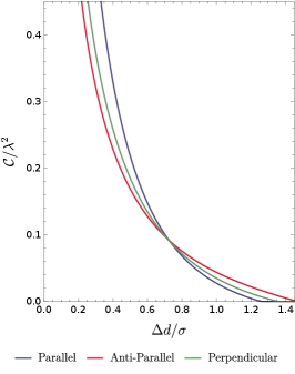
As shown in Fig.(10)/(11), the harvested entanglement in general decreases as either the acceleration or the detectors’ separation increases regardless of the acceleration scenario. Similar conclusions have also been reached in the case of the circular motion with nonlinear acceleration Zhjl:2020 . Interestingly, as the acceleration increases, the concurrence for the parallel acceleration case decreases faster than that for the anti-parallel acceleration and perpendicular acceleration cases when is not too small (e.g., or in Fig.(10)). While for a small , the concurrence for the parallel acceleration is generally larger than that for other acceleration scenarios (see in Fig.(10)). Therefore, when is not too small, the detectors in parallel-acceleration comparatively extract more entanglement from the fields over a certain range of relatively small values of . But the harvesting-achievable range of , in which the entanglement can be harvested successfully, may be shorter in the parallel-acceleration case than that in the anti-parallel acceleration and perpendicular acceleration cases. Another interesting feature is that for a very large acceleration, entanglement harvesting no longer occurs although the concrete value of acceleration when the harvesting ceases depends on the acceleration scenario. Qualitatively similar conclusions can also be drawn from Fig. (11) of the role of detectors’ separation in entanglement harvesting with fixed at certain values.
To further understand the influence of the presence of the boundary on the harvesting-achievable range of the separation and the acceleration in the parameter space where entanglement harvesting is possible, we define a new parameter to denote the maximum value of the acceleration , beyond which entanglement harvesting does not occur any more, and plot the dependence of and on the distance between the detectors and the boundary in Figs. (12) and (13) in all three acceleration scenarios.
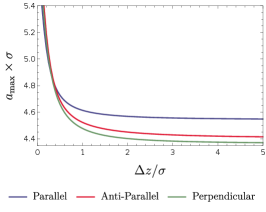
As we can see from these figures, and decrease with the increasing distance between the detectors and the boundary. In particular, the presence of the boundary could enhance the harvesting-achievable range of for detectors in acceleration or at rest. This means that the positive impact of the boundary on the harvesting-achievable range is irrespective of the detectors’ motion status. However, the quantitative details of differ slightly for different scenarios. As shown in Fig. (12), the inertial case has a comparatively larger than three acceleration scenarios for a certain fixed , which can be simply attributed to the negative impact of the thermal noise that arises from acceleration. When , and approach the corresponding values in the free spacetime without boundaries. Therefore, we conclude that the presence of the boundary enlarges the parameter space of and where the entanglement could be extracted successfully as compared to the case without a boundary, although it generally degrades the entanglement extracted by the accelerated detectors.
One can observe from Fig. (12a) that, for a small acceleration (), three solid curves approach the dashed curve, and this is expected since in the limit of , we should recover the inertial case with detectors at rest. Differences also show up for different acceleration scenarios. For a small acceleration, one can see that the parallel acceleration case has a larger than both anti-parallel and perpendicular acceleration cases, and the smallest is the anti-parallel acceleration case. Physically, this means that the parallel acceleration provides spacious “room” of separation for the detectors to extract the entanglement successfully, and the anti-parallel acceleration provides the least “room” for entanglement extraction. These properties are however inconspicuous in the regime near the boundary. Note that the dashed line, representing for two rest detectors, is always above the solid curves, which implies that acceleration always shortens the separation between the detectors that allows the entanglement harvesting to occur.
As acceleration grows, will decrease because of the increased thermal noise caused by the Unruh effect. However, the amount of the decrease differs for different acceleration scenarios so that when the acceleration is no longer small, the order of the magnitude of changes (see Fig. (12b) and Fig. (12c)). In place of the parallel acceleration, the anti-parallel acceleration now becomes the optimum choice that has the largest . This can be easily understood in the same way as we did for the comprehension of Figs. (8) and (9).
In Fig. (13), similar conclusion about can also be obtained. For a large , the anti-parallel acceleration has comparatively larger than both the parallel and perpendicular acceleration, which means that the case of anti-parallel acceleration has a larger range of acceleration for the detectors to harvest entanglement in the parameter space. However, for a small , the case of the parallel acceleration, especially in the region far from the boundary, is the optimum choice that has more “room” to achieve the entanglement harvesting. Meanwhile, in the region close to the boundary, the values of become considerably large, but the differences of among three acceleration scenarios become tiny.
It is worth emphasizing that in the limit of (i.e., location on the boundary plane), the corresponding Wightman function Eq. (III) approaches zero. As a result, the concurrence vanishes and does not depend on the parameters and . Then the definition of and would make no physical sense. In the concrete numerical evaluation for Fig. (12)/(13), is approximately treated as two detectors being located on the boundary plane and no further numerical calculation is actually performed. Of course, if we attempt to implement the numerical integration for , the vanishingly small integral and the possible oscillatory integrand with singularities should require extremely high precision and very long computing time. Here, we choose not to evaluate and for , since such an evaluation is not expected to qualitatively change our conclusions. For clarity, we summarize our main results in Table. (1)and (2) which follow.
| Harvested entanglement | Three acceleration scenarios | Rest case \bigstrut |
|---|---|---|
| Inhibited by the boundary for | Yes | Yes \bigstrut |
| Peaks at for a not large fixed | Yes, a comparatively smaller peak than the inertial case | Yes \bigstrut |
| Decreasing harvesting-achievable range of as increases | Yes | Yes, a comparatively larger harvesting-achievable range than the acceleration case \bigstrut |
| Decreases as increases for a fixed | Yes | Yes \bigstrut |
| Harvested entanglement | Parallel acceleration | Anti-parallel acceleration | Perpendicular acceleration \bigstrut |
|---|---|---|---|
| Degrades with increasing (acceleration ) for a large () at fixed | Most rapidly | Rapidly | More rapidly \bigstrut |
| The amount for a small (large) and at fixed | Most (least) amount | Least (most) amount | Medium amount \bigstrut |
| The harvesting-achievable parameter space of or | Largest (smallest) or for a fixed small (large) or | Smallest (largest) or for a fixed small (large) or | Medium or \bigstrut |
V conclusion
In this paper, we have explored the phenomenon of entanglement harvesting for a pair of inertial as well as uniformly accelerated UDW detectors near a perfectly reflecting boundary. Three different acceleration scenarios, i.e., parallel, anti-parallel and mutually perpendicular acceleration, are considered. We find that the presence of the boundary significantly influences on the entanglement harvesting of the accelerated detectors. As a whole, the reflecting boundary inhibits the transitions of detectors and nonlocal correlation of the fields so that the harvested entanglement would degrade when two detectors are close to the boundary. However, when the distance between detectors and the boundary is comparable to parameter which characterizes the interaction duration, the harvested entanglement may approach a peak, which even goes beyond that without a boundary. More interestingly, we find that the presence of the boundary, in all three acceleration scenarios, could enlarge the parameter space ( acceleration and detectors’ separation ) beyond which the entanglement harvesting no longer occurs. These conclusions also qualitatively hold for inertial detectors at rest.
A comparison of three different acceleration scenarios reveals that the entanglement harvesting crucially depends on the distance between the detectors and the boundary, the acceleration and the detectors’ separation. As far as the amount of the entanglement harvested is concerned, the detectors in parallel acceleration are likely to harvest the most entanglement in the case of a small acceleration or small detectors’ separation. However, those in anti-parallel acceleration may harvest the most entanglement in the case of a large acceleration and large detectors’ separation. For the parameter space that allows entanglement extraction to occur, we find that, for a vanishing small acceleration, the harvesting-achievable range of detectors’ separation for all three acceleration scenarios is basically the same near boundary. However, in the region far away from the boundary, the parallel acceleration is the optimum choice that has the largest detectors’ separation to achieve entanglement harvesting. While for a not too small acceleration, the anti-parallel acceleration becomes the optimum choice that has the largest separation. Similar conclusions can be obtained for the harvesting-achievable range of acceleration when entanglement harvesting is still possible with a certain fixed detectors’ separation. Also, our direct numerical calculation instead of the saddle approximation seems to indicate that acceleration always shortens the detectors’ separation that allows the entanglement harvesting to occur.
Finally, we have demonstrated how the presence of a boundary affects the entanglement harvesting for two uniformly accelerated detectors. We anticipate that these methods can be used to investigate the entanglement harvesting in other cases, such as two detectors with different magnitudes of acceleration or with acceleration along the normal direction of the boundary or even in curved background. It is quite a challenge to perform numerical evaluation due to the complexity of the issue. We would rather leave such studies to future works.
Acknowledgements.
This work was supported in part by the NSFC under Grants No. 11690034 and No.12075084; and the Research Foundation of Education Bureau of Hunan Province, China under Grant No.20B371.Appendix A Derivation of
To verify Eq.(III), let us begin from Eq. (4). Taking into consideration the fact that the Wightman function (III) for trajectory (8) is only a function of the difference between and and letting and , we have, after integrating firstly,
| (27) |
By inserting Eq. (8) into Eq. (A) and performing some simple algebraic manipulations, the transition probability can be written into two terms as
| (28) |
with the first term satisfying
| (29) |
and the second term
| (30) |
where and . can be rewritten as
| (31) |
In second line of the above equation, we have neglected the factor since the integral is now regular. While the second term can be re-expressed as
| (32) |
Here, we have used the following identity that arises from the successive differentiation of the Sokhotski formula,
| (33) |
In addition, recalling the definition of a distribution acting on a test function
| (34) |
we have the following identities for a distribution function EDU:2016-1 ; Bogolubov:1990
| (35) |
| (36) |
and
| (37) |
where denotes the principle value of an integral. Thus, by using Eq. (36) and Eq. (37), Eq. (A) can be further written in a simple form as
| (38) |
As for , it can be written as
| (39) |
where Eq. (33) and Eq. (37) have been considered in the last step. Combining Eqs. (A), (38) and (A), one can easily verify the expression of the transition probability given in Eq. (III).
References
- (1) R. Blume-Kohout, C. M. Caves, and I. H. Deutsch, Foundations of Physics 32, 1641 (2002).
- (2) C.H. Bennett and S. J. Wiesner, Phys. Rev. Lett. 69, 2881 (1992).
- (3) C. H. Bennett, G. Brassard, C. Crepeau, R. Jozsa, A. Peres and W. K. Wootters, Phys. Rev. Lett. 70, 1895 (1992).
- (4) A. K. Ekert, Phys. Rev. Lett. 67, 661 (1991).
- (5) A. Osterloh, L. Amico, G. Falci and R. Fazio, Nature 416, 608 (2002).
- (6) G. Vidal, J. I. Latorre, E. Rico and A. Kitaev, Phys. Rev. Lett. 90, 227902 (2003).
- (7) L. Amico, R. Fazio, A. Osterloh and V. Vedral, Rev.Mod. Phys. 80, 517 (2008).
- (8) L. Mandel and E. Wolf, Optical coherence and quantum optics (Cambridge University Press, Cambridge, U.K., 1995)http://dx.doi.org/10.1119/1.18450.
- (9) C. Weedbrook et al.,Rev. Mod. Phys. 84, 621(2012).
- (10) L. Bombelli, R. K. Koul, J. Lee and R.D. Sorkin, Phys. Rev. D 34, 373 (1986).
- (11) C. Callan and F. Wilczek, Phys. Lett. B 333, 55 (1994).
- (12) M. Srednicki,Phys. Rev. Lett. 71, 666(1993).
- (13) S. Ryu and T. Takayanagi, Phys. Rev. Lett.96, 181602(2006).
- (14) S.J. Summers and R. Werner, Phys. Lett. A 110, 257 (1985).
- (15) B. Reznik, A. Retzker, and J. Silman,Phys. Rev. A 71, 042104 (2005).
- (16) A. Valentini, Phys. Lett. A 91,153321 (1991).
- (17) B. Reznik, Foundations of Physics 33,33167 (2003).
- (18) G. L. Ver Steeg and N. C. Menicucci, Phys. Rev. D 79, 044027 (2009).
- (19) S. J. Olson and T. C. Ralph, Phys. Rev. Lett. 106, 110404 (2011).
- (20) B. L. Hu, S.-Y. Lin and J. Louko, Class. Quant. Grav. 29, 224005 (2012).
- (21) E. Martín-Martínez and N. C. Menicucci, Class. Quant.Grav. 29, 224003 (2012).
- (22) E. Martin-Martinez and N. C. Menicucci, Class. Quant. Grav. 31, 214001 (2014).
- (23) E. Martín-Martínez, E.G. Brown, W. Donnelly and A. Kempf, Phys. Rev. A 88, 052310 (2013).
- (24) Y. Nambu, Entropy 15, 151847 (2013).
- (25) A. Pozas-Kerstjens and E. Martín-Martínez, Phys. Rev. D 92, 064042 (2015).
- (26) E. Martín-Martínez, A. R. H. Smith and D. R. Terno, Phys. Rev. D 93, 044001 (2016).
- (27) E. Martín-Martínez and B.C. Sanders, New J. Phys. 18, 043031 (2016).
- (28) L. J. Henderson, R. A. Hennigar, R.B. Mann, A. R H. Smith and J. Zhang, Class. Quant. Grav. 35, 21LT02 (2018).
- (29) L. J. Henderson, R. A. Hennigar, R. B. Mann, A. R. H. Smith and J. Zhang, JHEP 05,178 (2019).
- (30) K. K. Ng, R. B. Mann and E. Martín-Martínez, Phys. Rev. D 97, 125011 (2018).
- (31) K. K. Ng, R. B. Mann and E. Martín-Martínez, Phys. Rev. D 98,125005 (2018).
- (32) J. Zhang and H. Yu, Phys. Rev. D 102, 065013 (2020).
- (33) G. Salton, R.B. Mann and N.C. Menicucci, New J. Phys 17, 035001 (2015).
- (34) Q. Xu, S.A. Ahmad and A.R.H. Smith, arXiv:2006.11301.
- (35) W. Cong, E. Tjoa and R.B. Mann, J. High Energy Phys. 06, 021 (2019).
- (36) W. Cong, C. Qian, M.R.R. Good and R.B. Mann, arXiv:2006.01720.
- (37) S.-Y. Lin, C.-H. Chou and B. L. Hu, Phys. Rev. D 78, 125025 (2008).
- (38) S.-Y. Lin and B. L. Hu,Phys. Rev. D 81, 045019 (2010).
- (39) M. Ahmadi, K. Lorek, A Checińska, A. R. H. Smith, R. B. Mann and A. Dragan, Phys. Rev. D 93, 124031 (2016).
- (40) P. T. Crochowski, K. Lorek and A. Dragan,Phys. Rev. D 100, 025007 (2019).
- (41) N. D. Birrell and P. C. W. Davies, Quantum Fields in Curved Space https://doi.org/10.1017/CBO9780511622632 (Cambridge University Press, Cambridge, U.K.,1984).
- (42) L. Rizzuto,Phys. Rev. A 76, 062114 (2007).
- (43) R. Messina, R. Passante,Phys. Rev. A 76, 032107 (2007).
- (44) Z. Zhu and H. Yu, Phys.Rev. A 82, 042108 (2010).
- (45) H. Yu and S. Lu, Phys. Rev. D 72, 064022 (2005) [erratum: Phys. Rev. D 73, 109901 (2006)].
- (46) H. Yu and Z. Zhu, Phys. Rev. D 74, 044032 (2006).
- (47) L. Rizzuto and S. Spagnolo, J. Phys.: Conf. Ser. 161, 012031 (2009).
- (48) H. Zhai, J. Zhang and H. Yu, Ann. Phys. (N. Y.) 371, 338 (2016).
- (49) J. Zhang and H. Yu, Phys. Rev. D 75, 104014 (2007).
- (50) S. Cheng, H. Yu and J. Hu, Phys. Rev. D 98, 025001 (2018).
- (51) W.K. Wootters,Phys. Rev. Lett. 80, 2245 (1997).
- (52) N. N. Bogolubov, A. A. Logunov, A. I. Oksak and I. T. Todorov, General Principles of Quantum Field Theory (Kluwer Acaciemic Publishers, Dordrecht, The Netherlands, 1990).