Entropy production and efficiency enhancement in quantum Otto engines operating at negative temperatures
Abstract
Cyclic classical and quantum thermal machines show higher efficiency when the strokes are carried out quasi-statically. Recent theoretical and experimental work on figures of merit for thermal machines show that they have an advantage when operating in environments with negative temperatures. In an experimental proof of concept [Phys. Rev. Lett. 122, 240602 (2019)], it was shown that quantum Otto engines operating at negative temperatures can exhibit a behavior in which the faster the cycle is carried out, the higher the efficiency. In this work, we make use of the concept of entropy production and friction work to explain this counterintuitive behavior, and we show that it only occurs when reservoirs have negative temperatures.
pacs:
05.30.-d, 05.20.-y, 05.70.LnIntroduction. In the 1950s, when the discussion about the existence of negative effective temperatures in spin systems began Purcell and Pound (1951); Ramsey (1956); Abragam and Proctor (1958, 1957); Landsberg (1959), the manufacture of devices operating in these environments was still in its early stages of development. At that time, Zemanski’s words were visionary: "Up to the present time, the only real use for systems at negative temperature has been in the rapidly expanding field of masers and lasers. Perhaps, in the future, experiments on heat mechanisms and refrigerators will be performed at negative temperatures. Then it will truly fun to be an engineer." In fact, very recent studies and experiments on the operation of devices such as heat engines in environments with negative effective temperatures show that these devices may have an advantage compared to when operating at positive temperatures. For example, thermal engines can have higher efficiency than classically expected de Assis et al. (2019); Xi and Quan (2017); Mendonça et al. (2020); Nettersheim et al. (2022); Bera et al. (2024) and autonomous refrigerators can reach lower temperatures than would be possible if only positive temperatures were taken into account Damas et al. (2023).
Since Carnot it is well known that carrying out a cycle in finite times produces internal friction, thus increasing the entropy of the system, which in turn is related to the dispersion of energy in the form of heat. Therefore, according to the common wisdom, the best way to not waste energy by friction is to perform the strokes gently. However, thermal machines operating in environments with negative temperatures can present unexpected and counterintuitive behaviors, such as the surprising effect that, for certain parameters, the efficiency of an Otto engine is inversely proportional to the cycle duration de Assis et al. (2019). This state of affairs raise the following questions (i) why efficiency enhances when entropy is produced? (ii) How to explain that the faster the process, the greater the efficiency? The present work aims to answer these two questions, expanding the analyzes and results in de Assis et al. (2019) to clarify where the advantage generated by the physics of negative temperatures comes from.
The model. In this paper, the Quantum Otto Heat Engine (QOHE) we consider consists of a two-level system (TLS) operating between a cold reservoir at a positive temperature and a hot reservoir that can be either at negative de Assis et al. (2019) or positive Peterson et al. (2019) temperature. The stages of the quantum Otto cycle that gives rise to this quantum heat engine are as follows (see Fig. 1):
Expansion and compression stages. During the expansion and compression stages, the Hamiltonian of the TLS changes from to and to , respectively, following the trajectories dictated by and , with . Here, is the Planck constant, is the frequency of the TLS, is the excited eigenstate of , and is the duration of both compression and expansion stages. At the beginning of the expansion and compression stages, the state of the TLS is and , respectively, with and , where is the Boltzmann constant and is the temperature of the cold (hot) reservoir. After evolving unitarily, the TLS reaches the state at the end of the expansion stage and at the end of the compression stage, in which , where is the so-called time-ordering operator.
Heating and cooling stages. At the heating and cooling stages, the TLS is weakly coupled to the hot and cold reservoirs, respectively, until the equilibration process concludes. Throughout these stages, the Hamiltonian of the TLS remains constant: during the heating stage and during the cooling stage. The initial state of the TLS in the heating and cooling stages are, respectively, and . Upon completing the equilibration process, the final state of the TLS is in the heating stage and in the cooling stage.
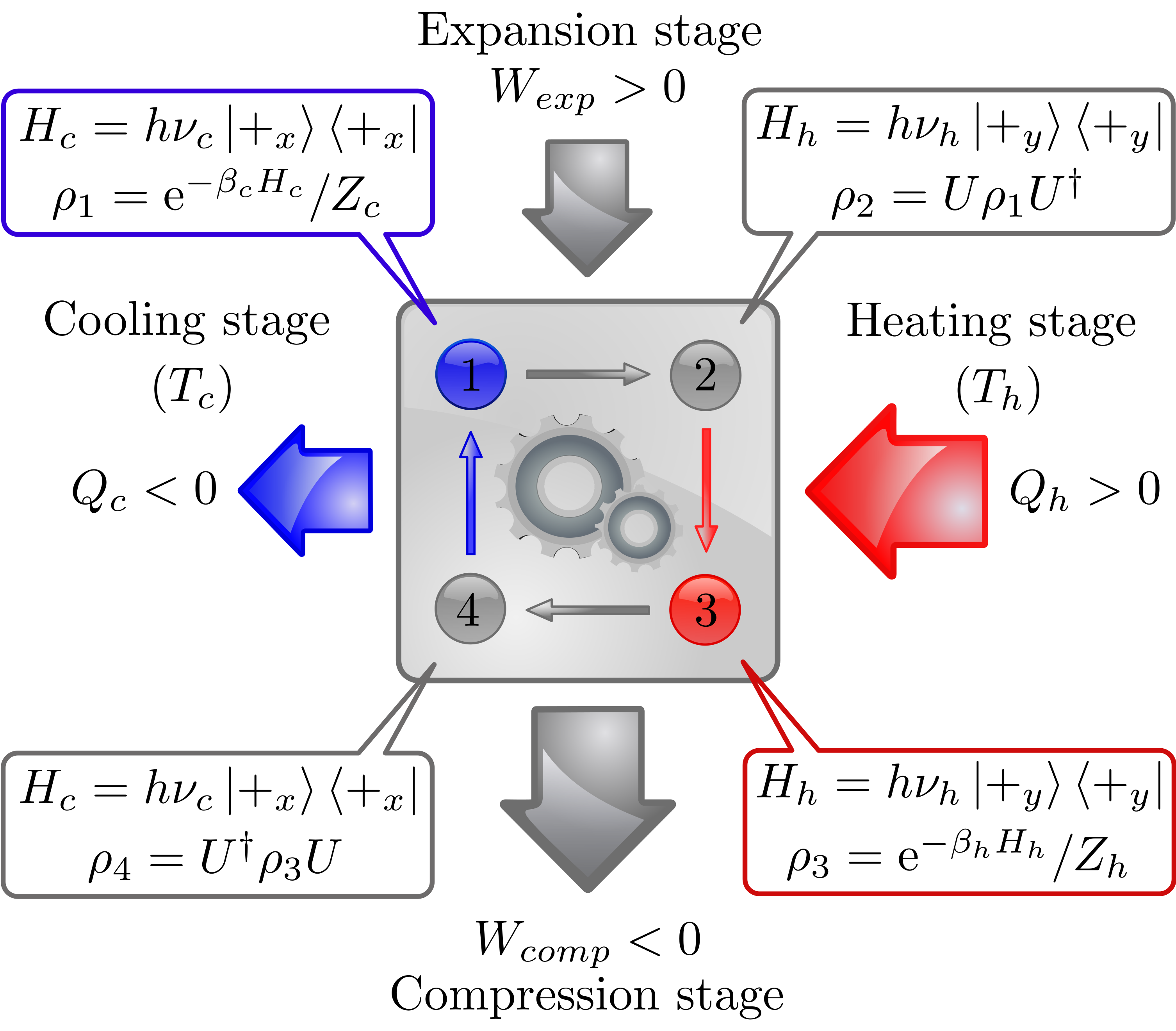
According to the definitions of work and heat introduced by Alicki in Ref. Alicki (1979), and , the exchange of energy throughout the compression and expansion stages occurs in the form of work, while it occurs in the form of heat during the heating and cooling stages. So, by calculating the energy variation of the TLS at each stage of the cycle ( and ), we obtain
| (1) |
| (2) |
| (3) |
and
| (4) |
In these expressions, we are always referring to the populations of the excited states: represents the population at the end of the cooling (heating) stage,
| (5) |
while corresponds to the transition probability between and in the compression (expansion) stage,
| (6) |
with being the ground eigenstate of .
Upon examining Eq. (5), we can easily see that is positive when and negative when . Therefore, a reservoir with a negative temperature inverts the population of the TLS.
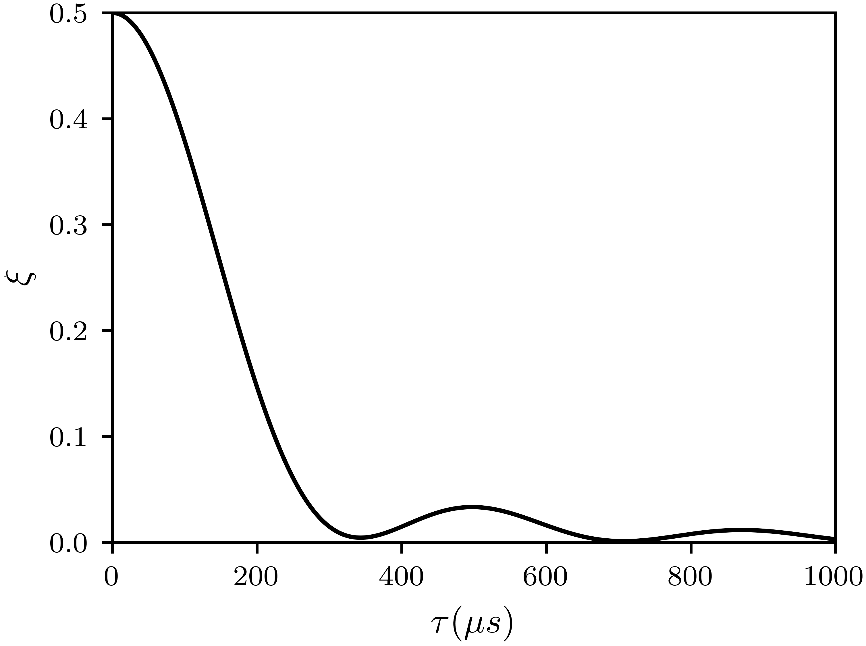
Due to the Hamiltonians and defined above, the transition probability is upper-limited by , reaching this limit when becomes the identity operator. In other words, as . The behavior of as a function of is shown in Fig. 2, in which we consider kHz and kHz. From this figure, we can also see that when , in accordance with the quantum adiabatic theorem, regardless of whether the system is in a population-inverted state or not.
Here we will use the convention according to which the quantum Otto cycle under consideration operates as a heat engine when , where is the network of the cycle, given by . By combining Eqs. (1) and (2), we obtain
| (7) |
The work performed can be divided into two distinct parts: and . The first part considers the quasi-static process, while the second part accounts for the work produced by internal friction, representing the extra work spent due to finite-time regimes. This occurs both in the presence of reservoirs at positive or negative temperatures. Therefore, the net work can be written as
The work produced by internal friction can be calculated using the Kulback-Liebler divergence, which is also related to entropy production as Plastina et al. (2014)
| (8) |
where stands for the relative entropy calculated between the states , which is the state at the end of the expansion (or compression) at finite-time, and , which describes the resulting state when the process is conducted adiabatically. After a straightforward calculation, we get
| (9) |
| (10) |
Notice that according to our convention, to extract work from the QOHE, we must have . From Eq. (8), we see that for positive temperatures the friction work is always positive, meaning that it enters Eq. (7) in a way that always reduces the useful work. On the other hand, from Eq. (9), we can see that the friction work, depending on the temperatures and operating frequencies of the engine, can contribute to either an increase or a decrease in useful work.
For a comprehensive analysis of the efficiency of the quantum Otto cycle, since the engine condition requires that be positive, and since the adiabaticity parameter is present in these two equations, we need to take into account the effect of this parameter on the ratio . Let us start by studying the condition for to be negative in Eq. (9), which is
| (11) |
Considering the case of negative temperatures, we observe that the populations of the excited states of the hot reservoir are contained in the interval , while for the excited states of the cold reservoir it is .
Since the frequencies and are fixed, we can select an appropriate range for and to satisfy Eq. (11). As a result, we obtain:
| (12) |
| (13) |
To assess the impact of friction on the efficiency , we will reframe it in relation to the populations of the excited states, based on our prior findings, Eq. (7) and Eq. (4). Once the conditions for the cycle to operate are met—namely, and —the efficiency is:
| (14) |
or simply:
| (15) |
Equation (15) enables us to examine the efficiency when the excited state populations and satisfy Eqs. (12) and (13). It is worth noting that the transition probability also influences the engine performance. Therefore, we can analyze the efficiency behavior for different durations of the expansion and compression stages. In cases where the process occurs adiabatically (), the efficiency corresponds to , which coincides with the efficiency of the ideal quantum Otto cycle operated between two reservoirs at positive temperatures. Comparing this with Equation (15), we can observe that to have , the following condition must be satisfied:
| (16) |
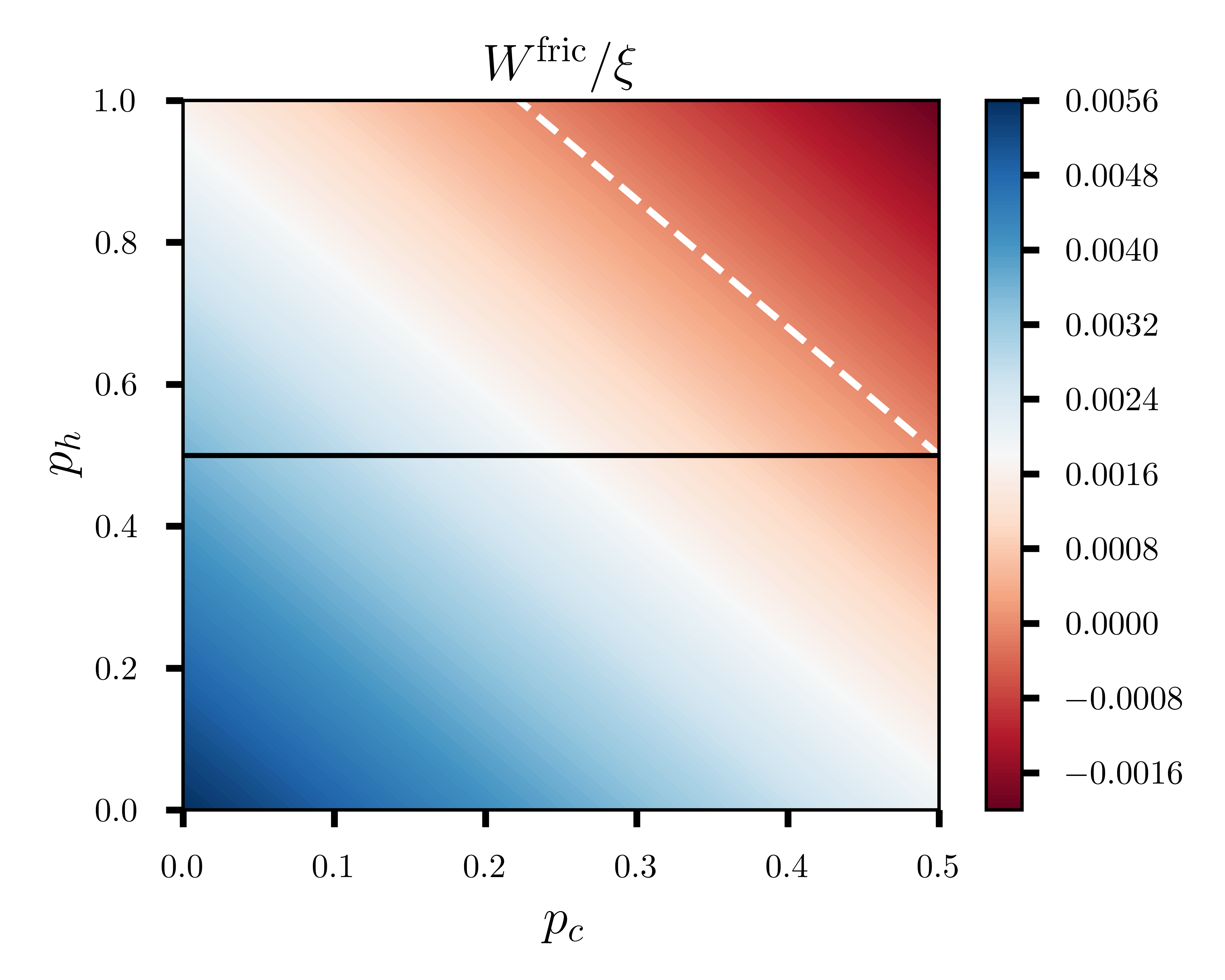
Results. Let us start by analyzing the friction work in two scenarios: with and without population inversion of the thermalized two-level system with the reservoir at temperature , which can be either positive or negative. In Fig. 3 we fixed and to plot the friction work versus the population of the excited state of the hot and cold reservoirs. These are the experimental frequency values used in Peterson et al. (2019); de Assis et al. (2019). The population inversion occurs for (above the black line), irrespective of the unitary stroke time duration. Note from Fig. 3 that the friction work can be both positive (below the white dashed line) and negative (above the white dashed line). When this work is null, precisely on the dashed white line, we have , indicating that the net work corresponds to what would be obtained in the adiabatic regime, even when executing the expansion and compression steps non-adiabatically. On the other hand, when the friction work is negative, it contributes to useful work, thus improving the engine efficiency. Interestingly, the population inversion of the hot reservoir, and thus negative temperatures, allows for processes where friction is null, regardless of the time at which the unitary steps are performed as evidenced in the region below the dashed white line in Fig. 3 when .
Let us now focus our attention on the net work, deepening our analysis of the Eq. (7). According to this equation, when the friction work is positive (as in the case of a cycle without population inversion), the amount of useful work extracted is smaller.
Positive temperatures. In the Fig. 4(a) we plot the net work versus the time duration of the unitary stroke in a cycle run with positive temperatures. Note the absence of the engine condition for . This absence of an engine regime occurs because, although the adiabatic work is negative in this regime, the friction work, which is larger due to entropy production at short times, prevails. In the Fig. 4(b) we show that the friction work is always positive, thus decreasing the net work. We also studied the absorbed heat , as shown in Fig. 4(c). It can be observed that for short times, . This is justifiable because, in Eq. (4), depending on the value of , the heat can assume negative values, violating the engine regime for this time interval. The corresponding efficiency is shown in Fig. 4(d). Note that the efficiency starts only for , which corresponds to the values of where the machine conditions are met. Also, observe that for values of , we have , approaching the adiabatic limit where the efficiency tends to . Given the chosen frequency values, this corresponds to .
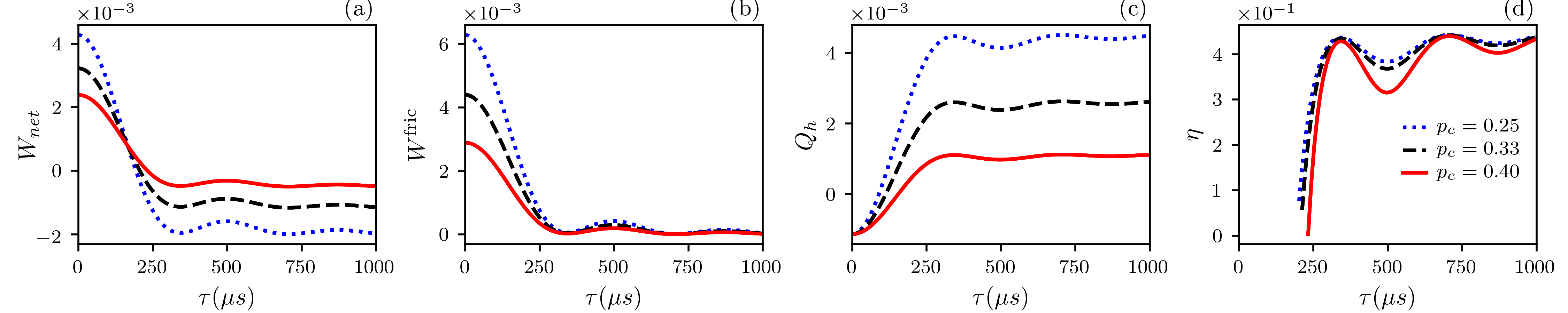
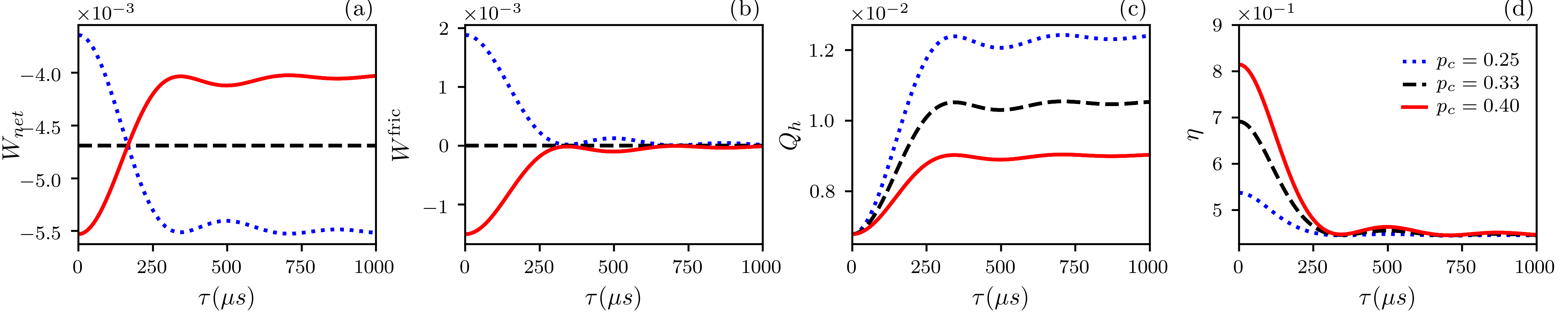
Negative temperatures. In Fig. 5(a) we show the net work versus the time duration of the unitary strokes. According to Eq. (12), a range of populations of the excited state of the cold reservoir exists for which the friction work is either negative or positive. For instance, with a fixed population of , selecting within the range results in negative friction work. Figure 5(b) illustrates this, with the dotted blue curve representing positive friction work and the solid red curve indicating negative friction work. Additionally, the dashed black curve denotes zero friction work, independent of . The presence of such a range where friction work is negative is significant, as it implies an algebraic addition of friction work in Eq. (7), leading to an increase in the amount of useful (negative) work extracted from the heat engine. Unlike the case of positive temperatures, the engine regime now exists for short times without restriction. When friction work is zero, the net work remains constant, corresponding solely to . Notably, from the red curve, we observe that the shorter , the more negative the net work, suggesting an increase in net work and an expected efficiency boost for short times. Furthermore, in Fig. 5(c), heat is depicted as a function of the unitary stroke time . Unlike the case with a positive hot reservoir temperature, is positive for all . This, combined with the fact that is also negative for all , ensures the engine condition is always met. Notably, in the regime of short times, absorbed heat progressively decreases until reaching a minimum. This occurs because the positive friction work produced in the expansion stroke, although greater for short times, leads to a subtraction of absorbed heat as per Eq. (4), resulting in increased efficiency. This efficiency increase for short times is evident in Fig. 5(d), where decreasing corresponds to increased efficiency. For all values, we observe , indicating that and satisfy Eq. (16). The solid red line represents the highest efficiency obtained (among tested values), corresponding to the case where friction work is negative, as seen in Fig. 5(b).
All the analyses conducted so far help us to understand the behavior of efficiency in the regime of negative temperatures. In fact, we have seen that when one of the reservoirs has a negative temperature, the terms associated with the finite-time regime appearing in the calculation of work and heat act to increase the net work extracted from the engine at the same time to reduce the amount of heat absorbed by the engine. Since efficiency is defined as , the appropriated choice for the populations , to result in always negative, allows the engine to achieve higher values for and lower values for , thus increasing the efficiency. Fig. 5(d) summarizes all the previous discussions on the behavior of work and heat exchanged between the working substance and the reservoir during the Otto cycle.
Conclusion. We conducted a study of the work and the heat of a quantum Otto heat engine operating in a finite time regime when one of the reservoirs presents negative temperature. By elucidating how the negative temperature environment modifies the heat and work exchanges between the engine and the reservoir due to the production of entropy during the unitary strokes performed at finite times, we explained the recently discovered counterintuitive phenomenon that, for certain parameters of the thermal engine, the efficiency enhances when entropy is produced, and even more counterintuitive, why the faster the process, the greater the efficiency of a heat engine.
Acknowledgements.
We are grateful to Rogério J. de Assis and Celso J. Villas-Boas for insightful discussions and suggestions. We acknowledge financial support from the Brazilian agencies: Coordenação de Aperfeiçoamento de Pessoal de Nível Superior (CAPES), financial code 001. This work was performed as part of the Brazilian National Institute of Science and Technology (INCT) for Quantum Information, grant 465469/2014-0.References
- Purcell and Pound (1951) E. M. Purcell and R. V. Pound, Physical Review 81, 279 (1951).
- Ramsey (1956) N. F. Ramsey, Physical Review 103, 20 (1956).
- Abragam and Proctor (1958) A. Abragam and W. Proctor, Physical Review 109, 1441 (1958).
- Abragam and Proctor (1957) A. Abragam and W. Proctor, Physical Review 106, 160 (1957).
- Landsberg (1959) P. Landsberg, Physical Review 115, 518 (1959).
- de Assis et al. (2019) R. J. de Assis, T. M. de Mendonça, C. J. Villas-Boas, A. M. de Souza, R. S. Sarthour, I. S. Oliveira, and N. G. de Almeida, Phys. Rev. Lett. 122, 240602 (2019).
- Xi and Quan (2017) J.-Y. Xi and H.-T. Quan, Communications in Theoretical Physics 68, 347 (2017).
- Mendonça et al. (2020) T. M. Mendonça, A. M. Souza, R. J. de Assis, N. G. de Almeida, R. S. Sarthour, I. S. Oliveira, and C. J. Villas-Boas, Physical Review Research 2, 043419 (2020).
- Nettersheim et al. (2022) J. Nettersheim, S. Burgardt, Q. Bouton, D. Adam, E. Lutz, and A. Widera, PRX Quantum 3, 040334 (2022).
- Bera et al. (2024) M. L. Bera, T. Pandit, K. Chatterjee, V. Singh, M. Lewenstein, U. Bhattacharya, and M. N. Bera, Physical Review Research 6, 013318 (2024).
- Damas et al. (2023) G. G. Damas, R. J. de Assis, and N. G. de Almeida, Physics Letters A 482, 129038 (2023).
- Peterson et al. (2019) J. P. Peterson, T. B. Batalhão, M. Herrera, A. M. Souza, R. S. Sarthour, I. S. Oliveira, and R. M. Serra, Physical review letters 123, 240601 (2019).
- Alicki (1979) R. Alicki, Journal of Physics A: Mathematical and General 12, L103 (1979).
- Plastina et al. (2014) F. Plastina, A. Alecce, T. J. G. Apollaro, G. Falcone, G. Francica, F. Galve, N. Lo Gullo, and R. Zambrini, Phys. Rev. Lett. 113, 260601 (2014).