Enumerating (multiplex) juggling sequences
Abstract
We consider the problem of enumerating periodic -juggling sequences of length for multiplex juggling, where is the initial state (or landing schedule) of the balls. We first show that this problem is equivalent to choosing ’s in a specified matrix to guarantee certain column and row sums, and then using this matrix, derive a recursion. This work is a generalization of earlier work of Fan Chung and Ron Graham.
1 Introduction
Starting about 20 years ago, there has been increasing activity by discrete mathematicians and (mathematically inclined) jugglers in developing and exploring ways of representing various possible juggling patterns numerically (e.g., see [1, 2, 3, 4, 5, 6, 10, 12, 14]). Perhaps the most prominent of these is the idea of a juggling sequence (or “siteswap”, as it is often referred to in the juggling literature). The idea behind this approach is the following. For a given sequence of nonnegative integers, we associate a (possible) periodic juggling pattern in which at time , a ball is thrown so that it comes down at time . This is to be true for each . Because we assume this is to be repeated indefinitely with period , then in general, for each and each , a ball thrown at time will come down at time . The usual assumption made for a sequence to be a valid juggling sequence is that at no time do two balls come down at the same time. This assumption results in many consequences, e.g., all of the quantities must be distinct, the number of balls in the pattern is the average , and the number of juggling sequences with period having fewer than balls is (see [1]).
An important object for understanding the relationships and transitions between various juggling sequences is the concept of a state diagram, developed independently (and almost simultaneously) by Jack Boyce and Allen Knutson [9]. This is a directed graph where each vertex is called a state or landing schedule, a - vector indicating when the balls that are currently in the air will land, and edges represent possible transitions between states. The vertex and edge sets for the state diagram can be defined as follows:
More specifically, each juggling sequence is associated with a state which can be found by imagining that the sequence has been executed infinitely often in the past, with a final throw being made at time . Then is if and only if there is some ball still in the air at time that will land at time . In this case we say that is a -juggling sequence.
If we are now going to throw one more ball at time , transitioning to a (possibly) new juggling state , then we are restricted to throwing it so that it lands at some time which has . The new state then has for and . The preceding remarks assume that . If , so that there is no ball available to be thrown at time , then a “no-throw” occurs, and the new state vector satisfies for all . These give the two basic transitions that can occur in the state diagram. With this interpretation, it is easy to see that a juggling sequence of period exactly corresponds to a walk of length in the state diagram.
In [5], the problem of enumerating -juggling sequences of period was studied, which by the above comments is equivalent to counting the number of directed closed walks of length starting at in the state diagram. In the same paper, the related problem of counting the number of “primitive” closed walks of length was also solved. These are walks in which the starting state is visited only at the beginning and the end of the walk.
A particular unsolved problem mentioned in [5] was that of extending the analysis to the much more complex situation of multiplex juggling sequences. In a multiplex juggling sequence, for a given parameter , at each time instance up to balls can be thrown and caught at the same time, where the balls thrown at each time can have different landing times. Thus, ordinary juggling sequences correspond to the case .
As before, we can describe a (multiplex) juggling sequence as a walk in a state diagram. Here a state can again be described as a landing schedule where are the number of balls currently scheduled to land at time . We also have a state diagram which has as its vertices all possible states and for edges all ways to go from one state to another state (see [10]). The state diagram is thus a directed graph with two important parameters: , the number of balls that are being juggled, and , the maximum number of balls that can be caught/thrown at any one time. The vertex set and edge set are defined as follows:
Since each state will only have finitely many nonzero terms, we will truncate the terminal zero portions of the state vectors when convenient. The height of a state will be the largest index for which , and will be denoted by . A small portion of the state diagram when and is shown in Figure 1.

1.1 A bucket approach
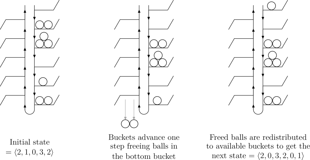
To better follow the analysis (and make practical demonstrations easier) we can reinterpret multiplex juggling by a series of buckets and balls. The buckets will represent future landing times for and the balls are distributed among these buckets. A state vector is then a listing of how many balls are currently in each bucket, and is now the maximum number of balls that can fit inside of a bucket. Transitions from state to state happen by having the buckets shift down by one and redistributing any balls that were in the bottom bucket. This process is shown in Figure 2.
1.2 Multiplex siteswap notation
To describe a walk in the state diagram it suffices to know what state we start in and how we transition from state to state. In transitioning from state to state the important piece of information is what happened to the ball(s) in the bottom bucket. This can be described by a multi-set which lists the new location(s) of the ball(s).
We can thus describe our walk by a series of multi-sets such that each set has elements (when we have fewer than balls to redistribute we will indicate no-throws by ). These sets are analogous to siteswap notation for juggling. In particular, it can be shown that
In the next section we will combine the idea of this multiplex siteswap notation with the buckets.
2 A matrix interpretation
One way to use the buckets to find a sequence of length that starts in state and ends in state (if one exists) is to start with the balls arranged in the buckets as dictated by . We then modify the capacities of the buckets so that they are (starting at the first bucket)
Finally, take steps (such as shown in Figure 2) being careful not to exceed the capacity of any bucket and at the end, we will be forced into state . On the other hand, every possible way to start in and end in in steps can be done in this modified buckets approach.
Finding all of the walks of length in the state diagram between and is thus equivalent to finding all of the walks that can be run using this modified bucket procedure. This is what we will actually enumerate. We start with the following matrix, where (this is a - matrix, where any unspecified entries are ’s).
![[Uncaptioned image]](https://cdn.awesomepapers.org/papers/b9359afd-d78d-4467-aa99-128c677ea002/x3.png)
Each block of columns will correspond to one transition in the state diagram/buckets procedure. In a block, each column corresponds to a single element in the multi-set describing our transition. The first in a column corresponds to a no-throw or a throw of height , the second corresponds to a throw of height , the third to a throw of height and so on. So we choose exactly one in each column and by reading the blocks of columns we will get the transitions between states.
Each row will correspond to a bucket, and to incorporate the modified buckets approach we specify a row sum for each row. The row sum will be the “unused capacity” of the buckets. Beginning at the first row and going down the row sums will be
As an example, suppose that we wanted a walk of length that starts and ends in the state in the state diagram shown in Figure 1. Then this corresponds to choosing one out of each column in the matrix below on the left so that the row sums are as dictated on the side of the matrix.
One possible solution is shown in the matrix on the right which corresponds to the walk
Here we have indicated the sets under each transition.
To see why this works we need to show that each multi-set given by a block of columns is a valid transition in our modified buckets procedure. Starting with the first block, the first row sum should be , this indicates that we currently have an excess capacity of in the bottom bucket and so we need to make no-throws, i.e., throws of height , and by row sum restrictions we are forced to select exactly of the ’s on the first row. This accounts for of the columns in the first block. The remaining columns must have ’s (i.e., balls) distributed among the rows (i.e., buckets) which still have extra capacity. Thus the first block must give a valid transition in the procedure. After selecting the ’s for the first block we then update the row sums according to our choices, remove the first block and then repeat the same process times.
Conversely, it is easy to check that given the transitions joining to , we can find a selection of ’s in the matrix which corresponds to this walk and satisfies the row/column sum restrictions.
Finally, since multi-sets are unordered, our choice of ’s in columns is unique up to permutation of the columns in a block, so we may assume that the heights of the ’s in a block are weakly decreasing (as shown in the example above). We now have the following general result.
Lemma 1.
Suppose we are given a state diagram with capacity and states and , and . Then the number of walks of length starting at and ending at is equal to the number of ways of choosing ones out of the matrix given above such that:
-
•
Each column sum is .
-
•
The row sums are (in order from first to last)
-
•
In each block of columns the height of selected ’s is weakly decreasing.
Remark 1.
If for some , , then one of the row sums will be negative which is impossible and thus we have no solutions for the selection of ’s. At the same time it is easy to see that there can be no walks in the state diagram of length joining and by comparing their landing schedules.
Remark 2.
When , if we ignore rows with row sum , then all the rows and column sums will be . In this case we can count the number of walks joining two states by calculating the permanent of a matrix. This is similar to the approach taken by Chung and Graham [5].
3 Filling the matrix
We now count the number of ways to fill the matrix according to the restrictions in Lemma 1. We will demonstrate the procedure by working through an example, namely counting the number of periodic multiplex juggling sequences of length that start and end in state when .
The first thing to observe is that when the height of is small compared to then the row sums have the following form:
We can form a recurrence based on this where we fill in the last block and then reduce it to the case when there is one fewer in the middle.
Without loss of generality we can assume that our noise at the end is a partition of the balls so that no part is larger than , i.e., we can ignore any rows with row sum and by a simple correspondence we can assume that the row sums are weakly decreasing.
For each partition of with each part at most , let be the number of ways to fill the matrix where the row sums are given by
In our example, there are such partitions, , and so we will have the three functions , and .
We now form a system of linear recurrences, , by examining the different ways to fill in the last block of columns. Note that the row sums corresponding to the last block are . The comes from the no-throws and after we have filled in the last block it will become incorporated into the new terminal distribution. Thus at each stage we will decrease the number of middle ’s by .
For example, if we are considering then we have the following different ways to fill in the last block satisfying the conditions of Lemma 1:
By looking at the new terminal distributions it follows that
Similar analysis shows that
We can rewrite this in matrix form as
| (1) |
In general, we will have that where as given above. Note that the matrix will be independent of our choice of and , and depends only on and . Varying will change the initial conditions and varying will change which of the we are interested in for our recurrence.
For our problem, we are interested in as our terminal state is (i.e., corresponding to the partition ). We want to transform our first-order system of linear recurrences into a single recurrence for . Manipulating the recurrences in (1) it can be shown that
| (2) |
This gives a recurrence for the number of periodic juggling sequence of length for sufficiently large (i.e., we have shifted our sequences past the initial noise; when counting periodic juggling sequences we need to remember to account for this shift).
Remark 3.
The characteristic polynomial of the matrix in (1) is , the same coefficients as in (2). This is a consequence of the Cayley-Hamilton Theorem. Namely if the characteristic polynomial of the matrix is then
The recursion that the characteristic polynomial of gives is universal for a fixed and in the following sense. Let be the number of walks of length joining state to state . Then for sufficiently large, satisfies the recursion given by the characteristic polynomial of (which is independent of and ).
It remains to calculate enough initial terms to begin the recursion. Using Lemma 1 this can be handled by brute force or some careful case analysis. In general, we will need to calculate the first terms where is the number of partitions of with each part at most . The first terms are to handle the initial noise caused by and the next terms are to help start the recursion. A calculation shows that the sequence counting the number of periodic juggling sequences that start and end at starts . Now applying the recursion we get the sequence
With the recursion and the initial values it is then a simple matter to derive a generating function for the number of juggling sequences of period . The generating function for this series and several others are given in Table 1.
| State | Initial terms | Generating Function | |
|---|---|---|---|
Remark 4.
Instead of calculating the first terms we can instead calculate the first terms and then compute the values for the . In at least one case this is easier, namely when the state is . Then it is easy to check that for all partitions and quickly bootstrap our sequence.
3.1 Calculating recursion coefficients
In this section we show how to quickly compute the recursion coefficients , which can then (by taking determinants) quickly give us the recursion relationship for the juggling sequences.
Lemma 2.
Let and be partitions of with no part more than , and suppose that and where is the number of parts of the partition of size , similarly for . Then
| (3) |
Proof.
To see (3) recall that when filling in the last set of columns of the matrix there is the partition and an additional row with row sum . We then select ones such that (1) the height of the ones are weakly decreasing and (2) no row sum is violated.
This process can be made equivalent to taking the partition and adding one part of size (to form a new partition ) then reducing by a total of some part(s) of .
The coefficient is then the total number of ways that reducing some part(s) of by a total of will result in the partition . We can however work backwards, namely if we want a desired partition from our reduction we can “insert” the desired partition into (i.e., associate each part of with some part of which is at least as large) and then finding the difference between the insertion and (which difference will sum to ) gives the reduction to use.
Thus is the total number of ways that we can insert into . We now enumerate by inserting the partition backwards, namely we insert the largest parts first and then work down. First note that here are parts of size to insert and they can be positioned into any of the parts of size , which can be done in
ways. There are then parts of size to insert and they can be positioned in any of the parts of size at least that have not yet been used, which can be done in
ways. This process then continues, so that in general there will be parts of size to insert and they can be positioned in any of the parts of size at least that have not yet been used, which can be done in
ways. Putting it all together then gives the result. ∎
As a check for, suppose , and , then (3) gives
To get a nonzero coefficient we must have so that and so that . Putting these in and simplifying we are left with
This can easily be verified by hand.
4 Remarks
4.1 Primitive juggling sequences
We have demonstrated a way to count the number of periodic juggling sequences of length which start and end in a given state . A related problem is counting the number of primitive periodic juggling sequences. These are special periodic juggling sequences with the extra condition that the walk does not return to until the th step. This can be done by the following observation of Chung and Graham [5] (see also [7, 8]): If is the number of periodic juggling sequences of length that start and end at and , then counts the number of primitive periodic juggling sequences of length that start and end at where
Applying this to the data in Table 1 we get the information about primitive juggling sequences given in Table 2. Only one of the sequences shown in Tables 1 or 2 was previously listed in [11].
| State | Initial terms | Generating Function | |
|---|---|---|---|
A related open problem is to find the number of prime juggling sequences which start and end in a given state . A prime juggling sequence corresponds to a simple cycle in the state diagram, i.e., it never visits any vertex more than once. Note that for a primitive juggling sequence we are allowed to visit vertices other than as often as we want.
4.2 Further directions
One implicit assumption that we have made is that the height the balls can be thrown to in the juggling sequence is essentially limited only by the period. This might be unrealistic when trying to implement the procedure for an actual juggler. In this case we would like to add an additional parameter which is the maximum height a ball can be thrown. While it is not difficult to adopt the matrix to handle this additional constraint, our recursion method will no longer work. For this setting, the simplest method might be to find the adjacency matrix of the (now finite) state diagram and take powers to calculate the number of walks.
Another implicit assumption that we have made is that the balls are identical, it is easy to imagine that the balls are distinct and then we can ask given an initial placement of balls and a final placement of balls how many walks in the state diagram are there. This problem is beyond the scope of the methods given here. However, Stadler [13] has had some success in this direction (using different methods than the ones presented here), he was able to derive an expression involving Kostka numbers enumerating the number of such sequences, as well as several other related sequences.
It would be interesting to know for each , and , which states have the largest number of (primitive) -juggling sequences of length . When , then it would seem that the so-called ground state does. However, for larger values of , it is not so clear what to guess.
As can be seen there are still many interesting open problems concerning the enumeration of multiplex juggling sequences.
References
- [1] J. Buhler, D. Eisenbud, R. Graham and C. Wright, Juggling drops and descents, Amer. Math. Monthly 101 (1994), 507–519.
- [2] J. Buhler and R. Graham, A note on the binomial drop polynomial of a poset, J. Combin. Theory Ser. A 66 (1994), 321–326.
- [3] J. Buhler and R. Graham, Juggling patterns, passing, and posets, Mathematical Adventures for Students and Amateurs, MAA Publications, (2004), 99–116.
- [4] F. Chung and R. Graham, Universal juggling cycles, preprint.
- [5] F. Chung and R. Graham, Primitive Juggling Sequences, to appear in Amer. Math. Monthly.
- [6] R. Ehrenborg and M. Readdy, Juggling and applications to -analogues, Discrete Math. 157 (1996), 107–125.
- [7] I. M. Gessel and R. P. Stanley, Algebraic enumerations, Handbook of Combinatorics, Vol. II, Elsevier, Amsterdam, (1995), 1021–1061.
- [8] R. L. Graham, D. E. Knuth and O. Patashnik, Concrete Math. A Foundation for Computer Science, Addison-Wesley, Reading, MA, (1994).
- [9] Juggling Information Service at www.juggling.org.
- [10] B. Polster, The Mathematics of Juggling, Springer, New York, 2000.
- [11] N. Sloane, Online Encyclopedia of Integer Sequences, www.research.att.com/~njas/sequences/.
- [12] J. D. Stadler, Juggling and vector compositions, Discrete Math. 258 (2002), 179–191.
- [13] J. D. Stadler, personal communication.
- [14] G. S. Warrington, Juggling probabilities, Amer. Math. Monthly 112, No. 2, (2005), 105–118.