EPIC229426032 and EPIC246067459 : discovery and characterization of two new transiting hot Jupiters from K2
Abstract
We report the discovery of two hot Jupiters orbiting the stars EPIC229426032 and EPIC246067459. We used photometric data from Campaign 11 and 12 of the Kepler K2 Mission and radial velocity data obtained using the HARPS, FEROS, and CORALIE spectrographs. EPIC229426032 and EPIC246067459 have masses of and , radii of and , and are orbiting their host stars in 2.18 and 3.20-day orbits, respectively. The large radius of EPIC229426032 leads us to conclude that this candidate corresponds to a highly inflated hot Jupiter. EPIC2460674559 has a radius consistent with theoretical models, considering the high incident flux falling on the planet. We consider EPIC229426032 to be a excellent system for follow-up studies, since not only is it very inflated, but it also orbits a relatively bright star ().
keywords:
planets and satellites: detection – planets and satellites: fundamental parameters – planets and satellites: gaseous planets1 Introduction
Since the detection of the first transiting exoplanet (HD 209458 b, Charbonneau et al., 2000), the anomalously large radii of many hot Jupiters have been puzzling astronomers trying to understand the formation and composition of these systems. Inflated giant planets have radii larger than what theoretical models predict for their masses (Burrows et al., 2007; Fortney et al., 2007), and are often found orbiting their host stars at short periods. This has led many groups to link planetary inflation with several effects, most importantly derived from their stellar insolation (for a review of these theories, see Weiss et al., 2013), and based on observational evidence, an insolation limit of has been set which can trigger the expansion of the planet (Miller & Fortney, 2011; Demory & Seager, 2011).
With the launch of the NASA Kepler space mission (Borucki et al., 2010), later renamed Kepler K2 due to the failure of one of its reaction wheels (Howell et al., 2014), the number of exoplanets detected has witnessed an exponential growth. Because ultracool dwarfs and gas giant planet more or less share a common radius, dynamical mass measurements are required to determine whether a transit signal originates from a planet or an ultracool dwarf. For single-planet systems, this is possible through the radial velocity method, which also provides the high resolution spectra required for the characterization of the host star and, in consequence, the planet.
Currently, researchers working in Chilean institutions have privileged access to state of the art instrumentation for follow-up observation of planetary candidates through radial velocity. This leaded us to create a Chilean-based K2 project (K2CL), focused on the task of selection of planetary candidates through photometry from the K2 mission, and later follow up using high resolution spectrograph. Exciting results have already been published since the project was started (see Espinoza et al., 2016; Brahm et al., 2016; Jones et al., 2017; Brahm et al., 2018).
In this work we report the discovery of two hot Jupiters, orbiting two dwarf stars that represent two different cases of the hot Jupiter-type planets. EPIC 229426032 is an 11.6 magnitude F star visible from the southern hemisphere (Table 1). It was observed during Campaign 11 of the K2 mission, and the planet was found to have a mass of , but a radius of , making it a highly inflated hot Jupiter. The next planet, EPIC 246067459 , was found using data from Campaign 12 of K2 to be orbiting a G type star. For this planet, we found a mass of , and radius of . Even though the planet is in the hot Jupiter regime and receives a flux above the inflation threshold, it does not show inflation characteristics.
This paper is organized as follows, in Section 2 we present the data obtained for each star, including photometric and spectroscopic observations. In Section 3 we analyze and derive the atmospheric parameters and obtain estimates for their stellar parameters such as age, mass, metallicity, effective temperature and rotational velocity. We also model both the radial velocity observations and the light curves, and derive the physical characteristics for each planetary system. In Section 4 we show the evidences which imply that EPIC229426032 corresponds to a highly inflated hot Jupiter, while EPIC246067459 appears to be consistent with a hydrogen/helium dominated planet with some metal content. Finally, in Section 5, we present a summary of our findings.
2 Data
| EPIC 229426032 | EPIC 246067459 | |
| Parameter | ||
| R.A. (J2000) | 16:55:04.5 | 23:10:49.042 |
| Dec. (J2000) | -28:42:38 | -07:51:27.00 |
| 12.19 0.07 | 14.61 0.10 | |
| 11.60 0.05 | 13.75 0.02 | |
| 10.51 0.02 | 12.46 0.03 | |
| 10.27 0.02 | 12.10 0.04 | |
| 10.22 0.02 | 12.03 0.03 | |
| Distance (pc) | ||
| Spectral type | F6V | G2V |
| Mass () | ||
| Radius () | ||
| Density () | ||
| Teff (K) | 6257 100 | 5630 78 |
| [Fe/H] | 0.14 0.05 | 0.34 0.04 |
| (cm s-2) | 4.24 0.10 | 4.11 0.07 |
| Age (Gyr) | ||
| (days) | 5.07 0.02 | |
| (km s-1) | 11.76 0.90 | 3.78 0.57 |
2.1 Photometry
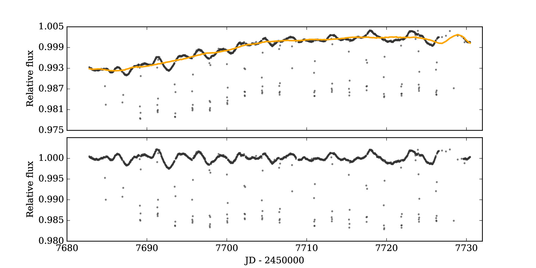
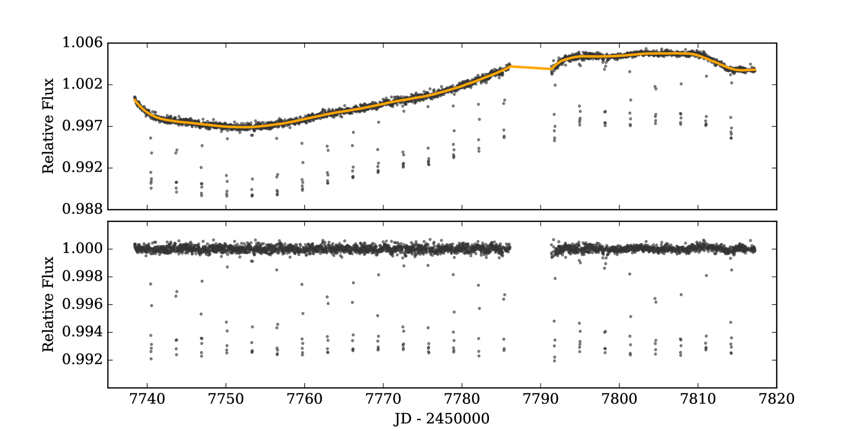
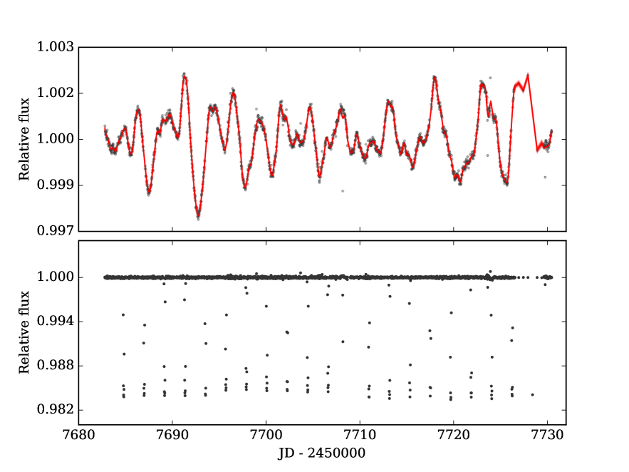
We analyzed photometric data from Campaign 11 (EPIC229426032) and Campaign 12 (EPIC246067459) of the K2 mission. We downloaded the Target Pixel Files (TPF) from MAST, extracted the photometry, and detrended it with an implementation of the EVEREST algorithm (Luger et al., 2017). The remaining long-term variations were removed following a similar procedure than the one described in Giles et al. (2018). We locally fit a third-order polynomial to sections of 0.5 days of the light curve, using a window of 10 days over the surrounding data. We repeat this process over the whole light curve. An outlier rejection was performed before fitting the data, to ensure that the transit was not removed. The light curves obtained after detrending and removing the long term variations are shown in Figs. 1 & 2. For the case of EPIC229426032, this is not the final light curve we used to derive the planet parameters. The data we used for that analysis is shown in Figure 6, and the process we followed to process it is explained in section 3.2.
2.2 Radial Velocity follow-up
Radial velocity follow-up data for EPIC229426032 was acquired using the CORALIE spectrograph (Queloz et al., 2000), mounted on the 1.2m Euler Swiss Telescope at La Silla Observatory.
We obtained 9 observations between July 7th and July 11th 2017. For each one of the 4 consecutive nights, we acquired two observations of 1800 seconds each, achieving a signal-to-noise (S/N) ratio of . The spectra were reduced and analyzed using the CERES automated pipeline (Brahm et al., 2017a). The mean radial velocity uncertainty achieved for this target was . The obtained radial velocities for each epoch are listed in Table 4.
We also acquired 4 additional radial velocity data points using HARPS (Mayor et al., 2003), which is mounted on the ESO 3.6m telescope at La Silla Observatory. The data were taken during four consecutive nights, with one 1800 seconds exposure per night. The S/N achieved for these data is . The observations were later processed using the CERES pipeline, obtaining an uncertainty in the radial velocities of . The HARPS velocities are listed in Table 5.
For EPIC246067459, 6 radial velocity measurements were obtained using FEROS (Kaufer et al., 1999), mounted on the 2.2m ESO/MPG Telescope at La Silla Observatory. The data was taken during five nights between November 6th and November 9th 2017, using exposures of 1500 seconds, and achieving S/N. The CERES automated pipeline was used to reduce and extract the radial velocities. The mean radial velocity uncertainty achieved with FEROS for this target is . The velocities are listed in Table 6.
2.3 High-resolution AO Imaging
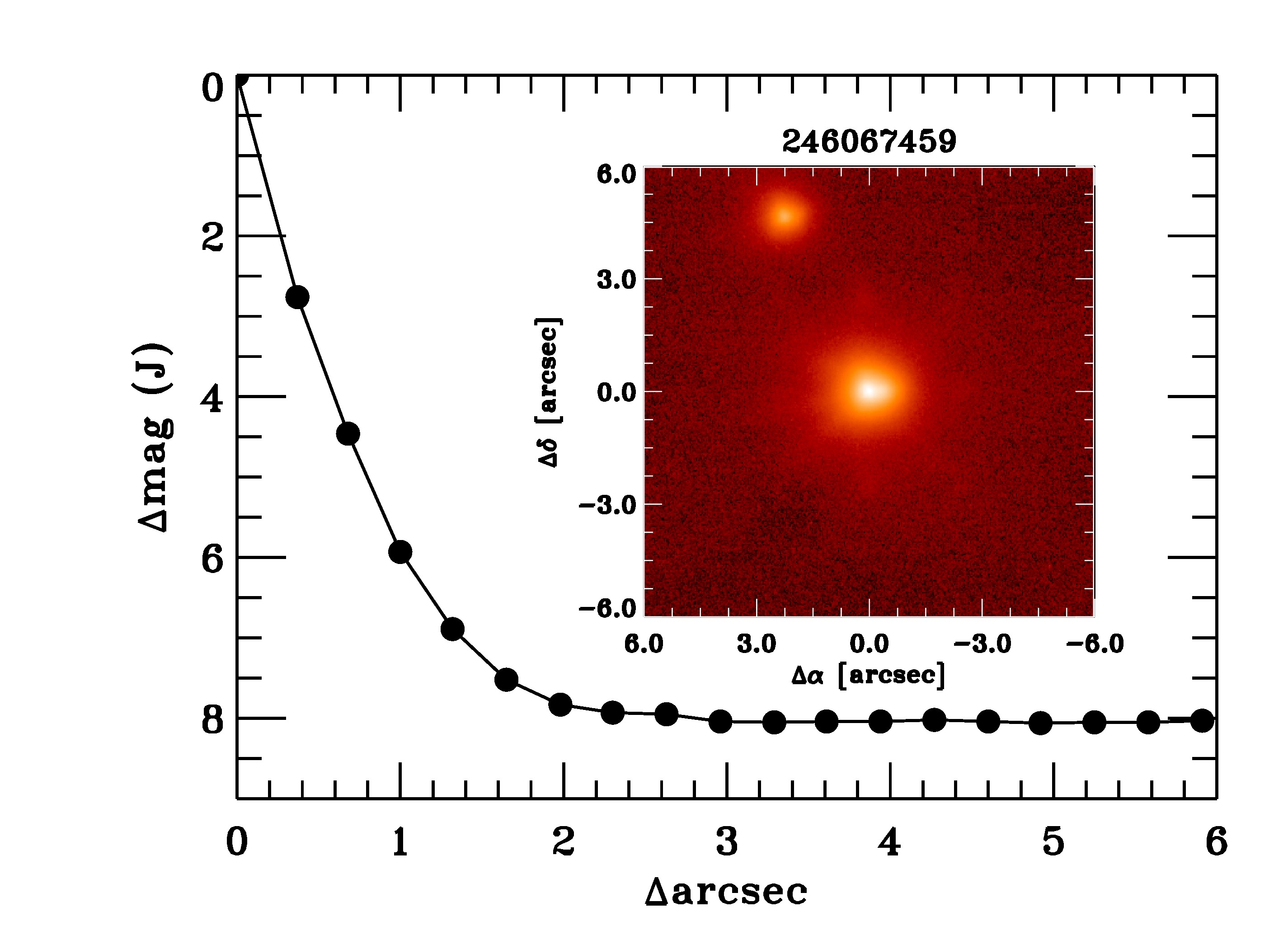
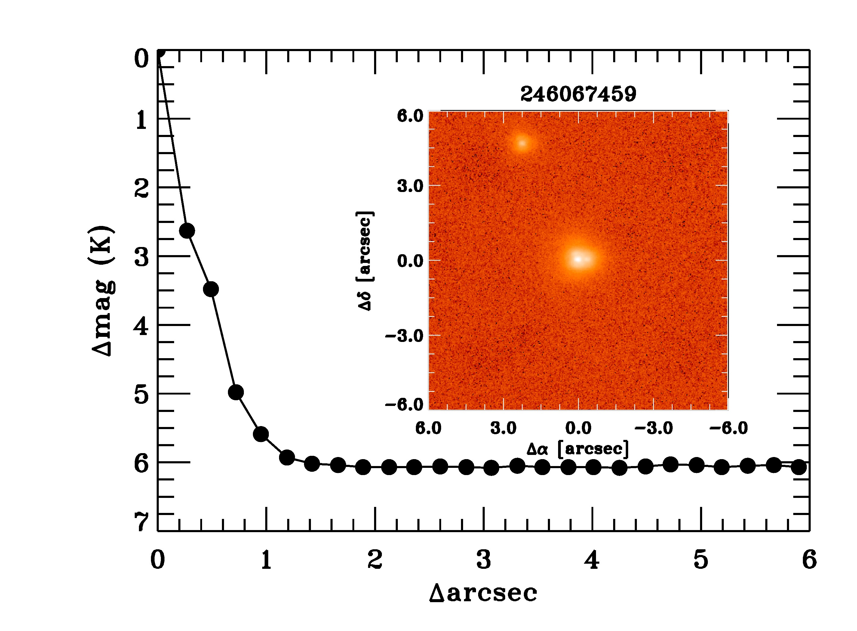
Observations on the and bands for EPIC 246067459 (Figure 3) were taken on August 30, 2017, using the ShaneAO (Gavel et al., 2014) at the Lick 3-m Shane Telescope. A PSF of 0.328” and 0.236” were obtained for the and bands, respectively. The contrast measured at 0.5” from the center is of and magnitudes for both bands, respectively. A companion star is seen in both images at around from our target (Figure 3).
The photometry was extracted for the resolved companion on both bands, with which we were able to estimate magnitude differences of and with respect to the brighter source, implying . Using this color, we use the Casagrande et al. (2010) color-temperature relations in order to derive a temperature of K for the resolved companion, where the error incorporates the uncertainty on the metallicity of the companion (propagated assuming an uniform distribution for it between the validity of the color-temperature relation), the error on our color estimation and the dispersion on the relation itself, which includes uncertainty on the unknown value of , and which assumes the companion is a dwarf or sub-giant star. We could also detect a second companion at 0.35” from our target. We used aperture photometry to deblend the K-band photometry, obtaining and for the primary star and the companion, respectively. Deblending in the J-band was not possible to perform.
Using the relations from Howell et al. (2012), we transformed the 2MASS photometry for both stellar companions to the Kepler bandpass, obtaining a magnitude difference with respect to our target of and , for the stars at 0.35” and 2.8” away, respectively. We estimate a dilution correcting factor of for the radius of the planet orbiting the primary star.
We do not find any close companions to EPIC 229426032 at 5” from the source.
3 Analysis
3.1 Stellar Parameters
The atmospheric parameters for both stars we computed using the Zonal Atmospheric Parameters Estimator (ZASPE, Brahm et al., 2017b) code. ZASPE matches the observed stellar spectrum with a set of synthetic spectra generated from the ATLAS9 (Castelli & Kurucz, 2004) model atmospheres. This procedure is performed via a global minimization, in a set of selected spectral regions. For EPIC229426032 we used the co-added CORALIE spectrum, after correcting each individual spectrum by its radial velocity. We used the CORALIE spectra, over the co-added HARPS spectrum, due to the higher S/N obtained. For EPIC246067459 we used the co-added FEROS spectra.
The physical parameters and evolutionary stages of both stars were obtained by interpolating through a grid of Yonsei-Yale isochrones (Demarque et al., 2004). We ran a Markov-Chain Monte Carlo (MCMC), using the emcee1 Python package, to explore the parameter space, given by the observed properties of each star. Using the metallicity value derived with ZASPE, we found the posterior distributions for the stellar age and mass. As observed parameters, we use the spectroscopic and the value obtained from the light curves (see section 3.3), which is a more precise proxy for the stellar luminosity than the spectroscopic (Sozzetti et al., 2007). The derived stellar parameters are listed in Table 1. Both stars have similar masses and are more massive than the Sun. While the parameters of EPIC 229426032 are consistent with being in the main sequence, the temperature, radius, and log(g) values of EPIC 246067459 show that it is slightly evolved. Additionally, both stars, in particular EPIC 246067459 ([Fe/H]=), are enriched in metals compared to the sun.
3.2 Rotational Period
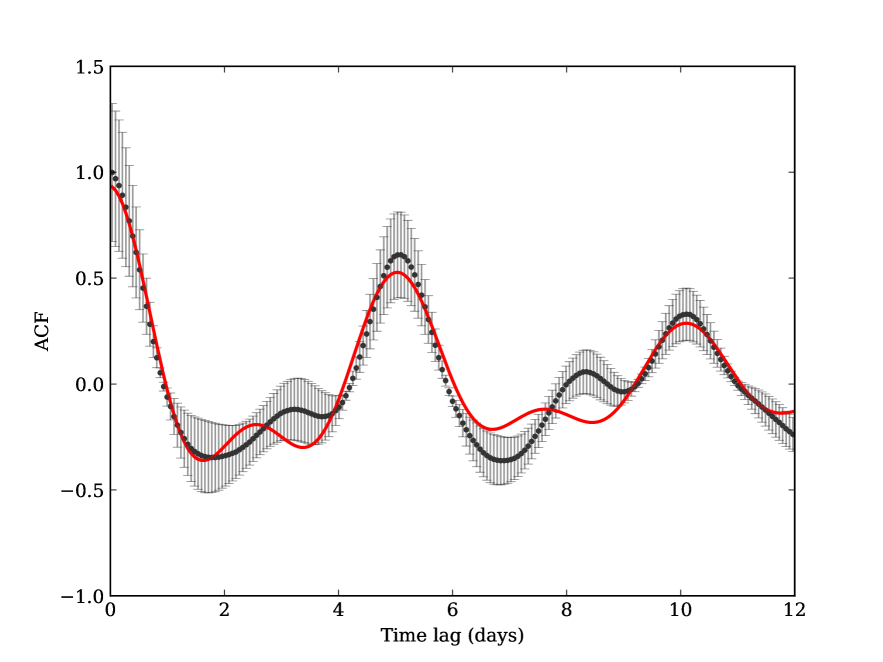
It is possible to measure the rotational period of a star from its light curve. If one assumes that the star’s surface contains spots blocking part of its flux, then a periodic signal will be produced and it can be detected in the light curve. This effect can be spotted in the data of EPIC229426032. The rotational period can be measured by using the autocorrelation function (ACF), which has been used with Kepler data in the literature (e.g. McQuillan et al., 2013; López-Morales et al., 2016; Giles et al., 2017). For this analysis we used the final light curve obtained from Section 2.1, after detrending and removing the long term variation.
We produced the ACF by following the method described in Edelson & Krolik (1988), using the implementation from astroML111http://www.astroml.org/modules/generated/astroML.time_series.ACF_EK.html. López-Morales et al. (2016) showed that the ACF follows a behavior similar to that of an under-damped simple harmonic oscillator (uSHO):
| (1) |
where is the decay timescale, is the rotation period, both in units of days, and is a constant.
We fit equation 1 to our ACF using a least-square minimization, and obtained the following solutions: days, days, , , and . Therefore, these results provide an rotational period of the star of days. The result is shown in Figure 4.
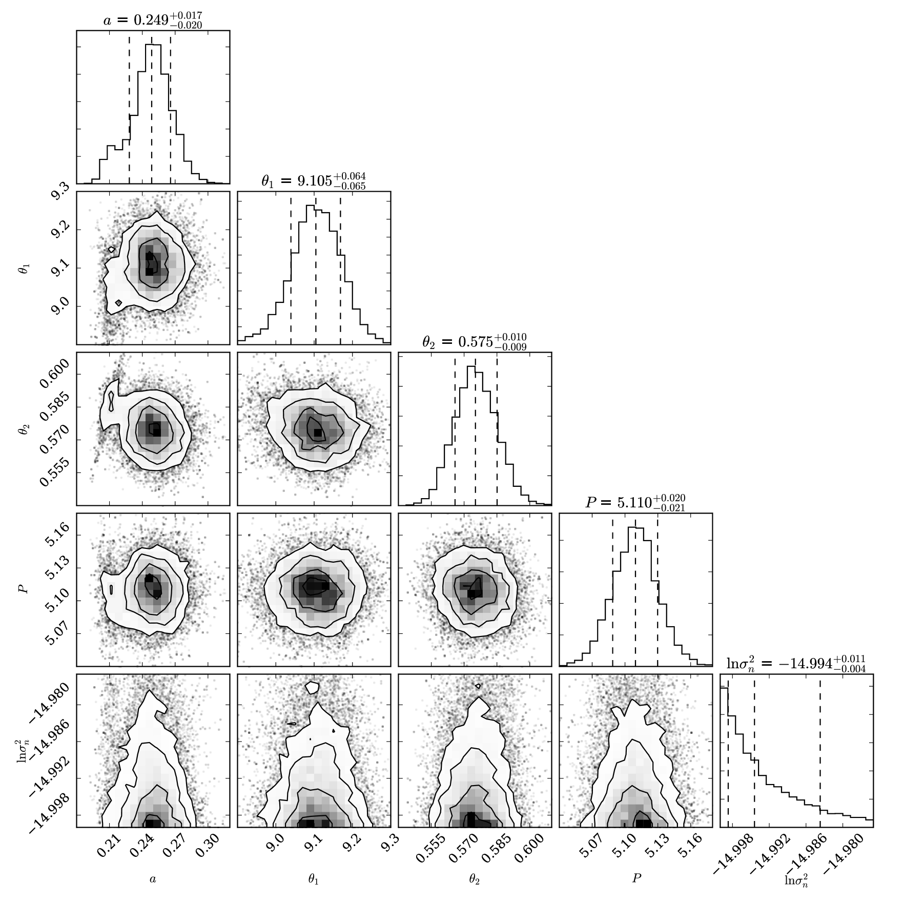
Before further analysis of the light curve to search for transit signals, we had to remove the effect of rotational modulation from the data. This was done through Gaussian Process (GP) analysis. Several works (e.g. Vanderburg et al., 2015; Aigrain et al., 2016; Angus et al., 2018) have shown that a Quasi-Periodic kernel can model sinusoidal variations in a dataset, with decay components. The Quasi-Periodic kernel is defined as:
| (2) |
where is the amplitude of the covariance function, is the time scale of the exponential decay, and are the amplitude and period of the sinusoidal component. We also included a white noise component to the kernel, of the form , where is the Kronecker delta. The values obtained from the ACF analysis were used as priors for and (Haywood et al., 2014; López-Morales et al., 2016). The amplitude was set to be constrained by the amplitude of the data, and to be within 0.05 and 5.0, following Jeffers & Keller (2009). The priors and best-fit values for each quantity are listed in Table 2.
| Parameter | Priora | Best-fit valueb |
|---|---|---|
-
a
represents a normal prior with with mean and standard deviation . represents a Jeffrey’s prior with limits and .
-
b
The values are shown as , where , and correspond to the 16, 50 and 84% percentiles.
We used the george222http://dan.iel.fm/george/current/ implementation of GP analysis, along with the emcee package, to adjust this kernel to our data by performing an MCMC sampling. The posterior distributions for each parameter of the Quasi-periodic kernel are shown in Figure 5. The final fit to the light curve is shown in Figure 6. The resulting light curve, without the effect of stellar rotation, was then used to derive the planet parameters for this star. Using the rotational period, with the stellar radius and the projected rotational velocity from Table 1, we obtain the rotational velocity and star inclination to be and degrees. For EPIC246067459, we could not measure the rotational period using this method because the signal by the stellar rotation embedded in the light curve was not as strong as with the other star.
3.3 Joint Analysis
| EPIC229426032 | EPIC246067459 | ||||
| Parameter | Unit | Priora | Best-fit valueb | Priora | Best-fit valueb |
| Period | days | ||||
| - 2450000 | days | ||||
| deg | |||||
| c | |||||
| c | |||||
| ppm | |||||
| fixed | fixed | ||||
| deg | fixed | fixed | |||
| - | |||||
| CORALIE jitter | - | ||||
| - | |||||
| HARPS jitter | - | ||||
| - | |||||
| FEROS jitter | - | ||||
| d | |||||
| g cm-3 | |||||
| AU | |||||
| K | |||||
| <>e | |||||
| f | cm | ||||
-
a
represents a normal prior with with mean and standard deviation . represents an uniform prior with limits and . represents a Jeffrey’s prior with limits and .
-
b
The values are shown as , where , and correspond to the 16, 50 and 84% percentiles.
-
c
and are the sampling coefficients to fit for a quadratic limb-darkening law, defined in Kipping (2013). The limb-darkening coefficients can be recovered as and .
-
d
The planet radius for EPIC246067459 considers the transit depth and the dilution produced by nearby stars (section 2.3). The uncorrected radius was found to be .
-
e
Orbit averaged incident flux.
-
f
Scale height, assuming hydrogen dominated composition.
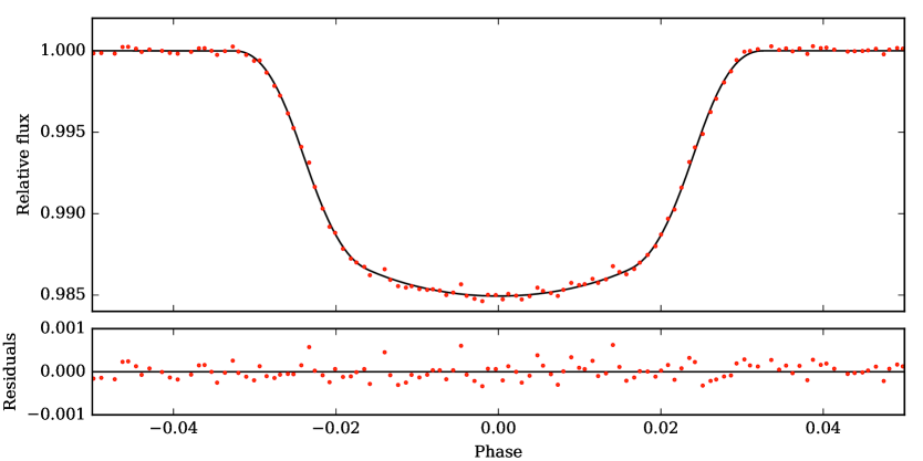
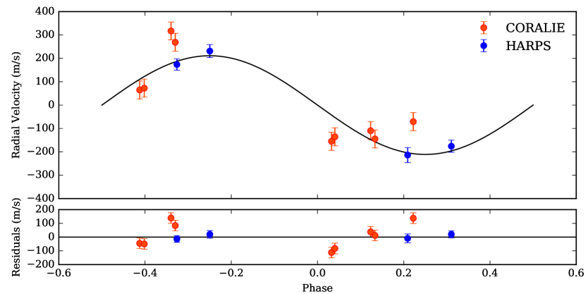
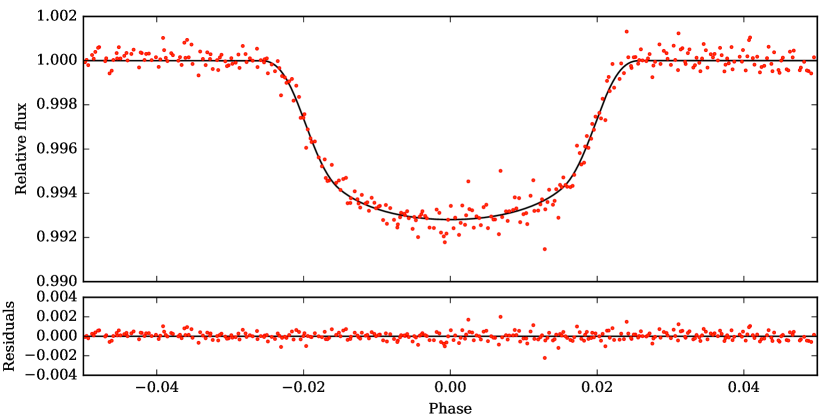
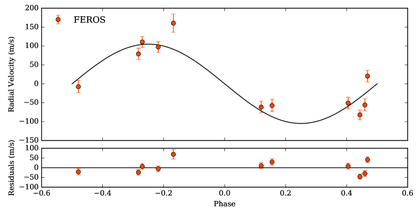
In order to obtain a global solution for both systems, combining the photometry and radial velocity information, we used the exonailer code (Espinoza et al., 2016). exonailer is a tool that fits transit light curves, as well as radial velocity information, using a Bayesian approach to derive the most probable solution, for a given system, by using a set of priors for each one of the orbital and transit model parameters. We used the quadratic limb-darkening law on both stars, which is the optimal one in our case following the algorithms and method detailed in Espinoza & Jordán (2016). We also fit for the limb-darkening coefficients instead of using modeled values, which has been shown to lead to important biases in the transit parameters (Espinoza & Jordán, 2015). We fitted the data of EPIC229426032 with both circular and non-circular models, and obtained that the eccentricity of the non-circular model was consistent with zero. The Bayesian Information Criterion (BIC) obtained for the circular orbit (BIC = -20.54) was also smaller compared with the non-circular one (BIC = -15.17), leading us to finally adopt a circular orbit for the system. The same analysis was done for EPIC246067459, where we also adopted a circular model. The obtained distributions for each parameter, as well as the limb-darkening sampling coefficients, are listed in Table 3. For EPIC229426032, we used the light curve obtained in section 3.2, and shown in the bottom panel of Figure 6, with the effect of stellar rotation and long term variations removed. For EPIC246067459, we used the detrended light curve obtained in section 2.1, and shown in the bottom panel of Figure 2. The transit and radial velocity solutions, given the posterior values from Table 3, are shown in Figure 7 and 8 for EPIC229426032 and EPIC246067459, respectively.
Using the stellar mass and radius computed in Section 3.1, along with the values from Table 3, we estimate the planet mass and radius to be and , respectively, for EPIC229426032 . For EPIC246067459 , we also had to consider the dilution in the transit depth produced by the two detected nearby companions. After correcting by this factor, we found the planet mass and radius to be and , respectively. These quantities, along with other parameters, are summarized in Table 3.
3.4 Activity indicators
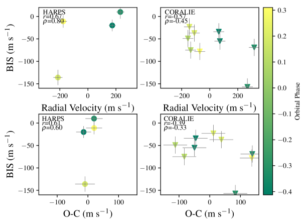
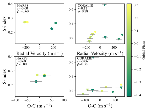
We measured a set of stellar activity indicators for both stars, in order to further confirm the planetary nature of the transit and radial velocity signals. For EPIC229426032, we measured the Bisector Inverse Span (BIS, Queloz et al., 2001; Toner & Gray, 1988), and the Ca ii H and K S-index (Jenkins et al., 2008; Jenkins et al., 2011). We used two coefficients to determine the level of correlation between the activity indices and the radial velocities for each instrument, the Pearson () and Spearman () correlation coefficients. For both quantities, the standard limits set for weak, moderate, and strong correlation between two quantities are , , and , respectively.
For the HARPS data, we obtain , and , for the correlation between the BIS and the S-index with the RVs, respectively (Figure 9). These results would suggest that both coefficients are correlated with the RVs, but the number of points considered is too small to make any robust conclusions. We performed the same analysis with the residuals from the planetary fit (see Figure 7), and obtained , and . This would also hint again at correlation with the activity indices, but as before, the number of points is too low to conclude whether this means there is moderate correlation between the quantities or not.
For the Coralie data, we find , and . For the BIS, the coefficients would suggest weak to moderate correlation with the RVs. We find that this correlation is powered only by one point (RV = 270 m s-1, BIS = -157 m s-1), and if we remove it, the correlation drops to . This reality is confirmed by a jacknife-like analysis that moved through the data, removing individual points and re-performing the correlation tests, highlighting that only when this outlying data point is removed does the correlation coefficient change. Too much statistical weight is being given to this one outlier. In fact, when we combine the HARPS and Coralie measurements, the coefficients also drop into the weakly correlated category, showing that stellar activity may be impacting the RVs, but only by adding random noise.
In the case of the correlation with the residuals from the planet fit we obtain , and , which indicates no correlation among these quantities. These results, for the HARPS and Coralie data, can be seen in Figure 9, with the activity indices listed in Table 4 and 5.
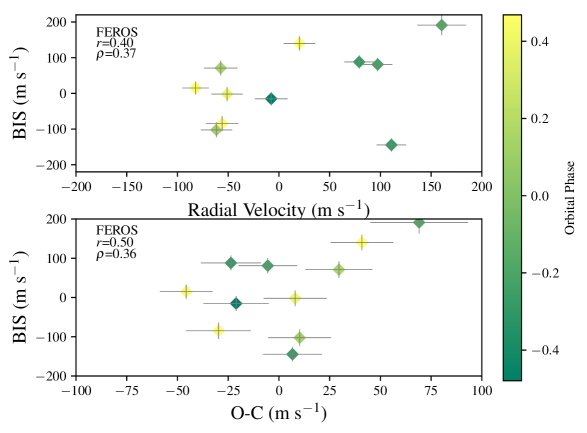
We also performed the bisector analysis on EPIC246067459, and found , which would indicate no correlation between the BIS and the FEROS RVs. For the residuals we found , also indicative of no strong correlation. The results are shown in Figure 10, and listed in Table 6. We did not include the S-index due to the low S/N spectra obtained with FEROS, which prohibited us from measuring them reliably.
3.5 Planet scenario validation
In order to confirm the planetary nature of our photometric and spectroscopic measurements, we performed a blend analysis using the algorithms described in Hartman et al. (2011b, a), which model the observations taking into account the possibility that they could be generated by either a planet, stellar companions physically associated with our target star or by various blend scenarios, including blended eclipsing binary and hierarchical triple systems.
EPIC 229426032b is confirmed to be a planet based solely on the photometry; it is practically impossible for the best-fit blend scenarios to fit the observed photometry in any of the cases consistent with the spectroscopic information. For EPIC 246067459b, the planetary interpretation is also favored by the data: although there is a detected close-by companion in the Lick 3m AO data, the lightcurve is not consistent with the transit/eclipses arising from the neighbor, as all the simulated lightcurve signatures imply colors much less than the observed . Considering that the brighter source could still itself be a blend, we can reject all the blend scenarios at 2.5 sigma-confidence based on the photometry. However, none of them are able to produce the observed m/s sinusoidal RV variation. The best-fit blend scenarios to the photometry also yield large bisector span variations in excess of 1 km/s, which are clearly ruled out by our measurements (see Figure 10). We consider thus both planets to be statistically validated given our photometric and spectroscopic measurements.
3.6 Searching for additional signals in the photometry
We search for additional signals in our K2 light curves, produced by other companions, orbital phase variations, or secondary eclipses by performing a Box-fitting Least Squares periodogram (BLS, Kovács et al., 2002) on the light curves, with the transits of the detected planets removed. We find no significant peak in the BLS for both stars, which limits the transit depth of the possible additional companions to be less than 220 ppm and 250 ppm for EPIC229426032 and EPIC246067459, respectively, for a detection. We could not detect secondary eclipses in neither of the light curves. For EPIC229426032 we had placed an upper limit for the depth of the eclipse to be ppm, so the fact that we could not detect it points to a geometric albedo of . This is in agreement with what has been found for hot Jupiters (Heng & Demory, 2013; Esteves et al., 2015). For EPIC246067459, it comes to no surprise that we could not detect its eclipse, given that its depth would have been ppm, which is bellow the detection limit of the data. We could not detect orbital phase variations in neither of the light curves.
4 Discussion
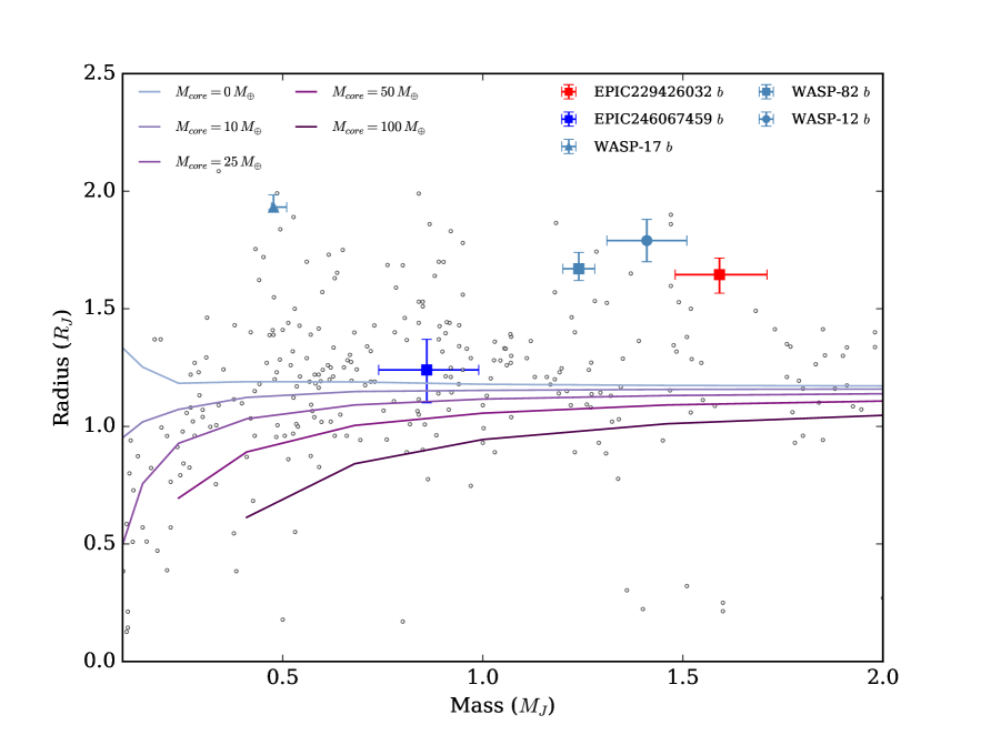
We compared the mass and radius of both planets with the models from Fortney et al. (2007), for hydrogen-helium dominated planets, with different amounts of metal compositions (represented by the core mass). We found for EPIC229426032 that the radius is significantly higher than expected for the given mass (0.5 larger than the model for a 4.5 Gyr-old planet with semi-major axis of 0.02 AU and no core). This is shown in Figure 11. We looked at the confirmed planets list from the NASA Exoplanet Archive333https://exoplanetarchive.ipac.caltech.edu/index.html, and found that EPIC 229426032 falls into a region of highly inflated hot Jupiters that is as yet not very well populated. We also compared the planet with other cases of highly inflated hot Jupiters, like WASP-17 (Anderson et al., 2010), WASP-82 (West et al., 2016), and WASP-12 (Hebb et al., 2009). These planets have shown to be good cases to perform atmospheric studies, which makes EPIC 229426032 a good laboratory for studying the atmospheres of highly inflated planets as well. For EPIC 246067459 , we find its radius to be consistent with the models of Fortney et al. (2007) for a hydrogen and helium dominated planet with a core mass up to 25 , at the level.
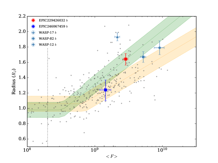
As was mentioned in the introduction, some studies trying to detect the source of planetary inflation point at correlations between the planet’s incident flux and radius (e.g. Demory & Seager, 2011; Laughlin et al., 2011), and have detected an incident flux threshold , above which inflation is found to happen. Both of our planets fall above this threshold as shown in Figure 12, which suggests inflation is shaping the observed radius of our newly discovered exoplanets. We see that EPIC 229426032 b is considerably larger than what theoretical models predict for a H/He dominated planet, receiving high radiation levels. In the case of EPIC 246067459 , its mass and radius seem to be consistent with it not-being inflated, even though it receives a high incident flux (Fig. 12). We also compared the two planets from this work with the models of radius against incident flux and mass by Sestovic et al. (2018). Here we see again see that EPIC 229426032 b appears to be even more inflated than what the model from Sestovic et al. (2018) predicts (, orange area in Figure 12). We also find that the scale height estimated for this planet (see Table 3) is comparable to those of systems currently targeted for atmospheric characterization (e.g., WASP-12b, with km, Burton et al., 2015). The latter, and given that the planet orbits a bright host star, again makes EPIC 229426032 b appear to be an excellent candidate for follow-up studies. For EPIC 246067459 , we see that its radius is consistent with a non-inflated planet of mass within within (represented by the flat part of the green region in Figure 12).
Jenkins et al. (2017) show that gas giant planets with orbital periods less than 100 days orbit stars that are significantly more metal-rich than their counterparts that host longer period giant planets. Furthermore, they also discovered a difference in the host star metallicity of Jupiter-mass planets and super-Jupiters, whereby the Jupiter-mass planets orbit stars significantly more metal-rich than those with significantly higher masses. This result was later confirmed at higher statistical significance by Santos et al. (2017). The very short period systems detected in this work also seem to orbit very metal-rich stars, and although the less massive of the two, EPIC226067459 , is still classed as a Jupiter-mass gas giant for the purposes of the metallicity-mass relationship discovered by Jenkins et al., it is intriguing that it orbits a significantly more metal-rich star than EPIC229426032 .
5 Summary
We present the discovery of two new hot Jupiters from our Chilean K2 project that aims to detect new planets in the southern fields of the K2 mission. For EPIC229426032 , our best solution is consistent with a hot Jupiter planet with a , orbiting its host star in a period of 2.2 days. Its radius makes it a highly inflated hot Jupiter, and when coupled with the brightness of the host, it makes an excellent candidate for further atmospheric studies.
EPIC246067459 , on the other hand, appears to have a mass similar to that of Jupiter, a radius of , and orbital period of 3.2 days. Even though this planet is in the regime where planetary inflation is important, it was found to have a radius consistent with theoretical models for H/He dominated objects.
Acknowledgements
MGS acknowledges the support of CONICYT-PFCHA/Doctorado Nacional-21141037, Chile. MRD is supported by CONICYT-PFCHA/Doctorado Nacional-21140646, Chile. JSJ acknowledges support by FONDECYT grant 1161218 and partial support by CATA-Basal (PB06, CONICYT). A.J. acknowledges support from FONDECYT project 1171208, BASAL CATA PFB-06, and by the Ministry for the Economy, Development, and Tourism’s Programa Iniciativa Científica Milenio through grant IC 120009, awarded to the Millennium Institute of Astrophysics (MAS). H.D. acknowledges support from FONDECYT Postdoctorado 3150314 and FONDECYT Regular 1171364, from Fondo Nacional de Desarrollo Científico y Tecnológico. R.L. acknowledges support from BASAL CATA PFB-06.
References
- Aigrain et al. (2016) Aigrain S., Parviainen H., Pope B. J. S., 2016, MNRAS, 459, 2408
- Anderson et al. (2010) Anderson D. R., et al., 2010, ApJ, 709, 159
- Angus et al. (2018) Angus R., Morton T., Aigrain S., Foreman-Mackey D., Rajpaul V., 2018, MNRAS, 474, 2094
- Borucki et al. (2010) Borucki W. J., et al., 2010, Science, 327, 977
- Brahm et al. (2016) Brahm R., et al., 2016, PASP, 128, 124402
- Brahm et al. (2017a) Brahm R., Jordán A., Espinoza N., 2017a, PASP, 129, 034002
- Brahm et al. (2017b) Brahm R., Jordán A., Hartman J., Bakos G., 2017b, MNRAS, 467, 971
- Brahm et al. (2018) Brahm R., et al., 2018, MNRAS,
- Burrows et al. (2007) Burrows A., Hubeny I., Budaj J., Hubbard W. B., 2007, ApJ, 661, 502
- Burton et al. (2015) Burton J. R., Watson C. A., Rodríguez-Gil P., Skillen I., Littlefair S. P., Dhillon S., Pollacco D., 2015, MNRAS, 446, 1071
- Casagrande et al. (2010) Casagrande L., Ramírez I., Meléndez J., Bessell M., Asplund M., 2010, A&A, 512, A54
- Castelli & Kurucz (2004) Castelli F., Kurucz R. L., 2004, ArXiv Astrophysics e-prints,
- Charbonneau et al. (2000) Charbonneau D., Brown T. M., Latham D. W., Mayor M., 2000, ApJ, 529, L45
- Demarque et al. (2004) Demarque P., Woo J.-H., Kim Y.-C., Yi S. K., 2004, ApJS, 155, 667
- Demory & Seager (2011) Demory B.-O., Seager S., 2011, ApJS, 197, 12
- Edelson & Krolik (1988) Edelson R. A., Krolik J. H., 1988, ApJ, 333, 646
- Espinoza & Jordán (2015) Espinoza N., Jordán A., 2015, MNRAS, 450, 1879
- Espinoza & Jordán (2016) Espinoza N., Jordán A., 2016, MNRAS, 457, 3573
- Espinoza et al. (2016) Espinoza N., et al., 2016, ApJ, 830, 43
- Esteves et al. (2015) Esteves L. J., De Mooij E. J. W., Jayawardhana R., 2015, ApJ, 804, 150
- Fortney et al. (2007) Fortney J. J., Marley M. S., Barnes J. W., 2007, ApJ, 659, 1661
- Gavel et al. (2014) Gavel D., et al., 2014, in Adaptive Optics Systems IV. p. 914805 (arXiv:1407.8207), doi:10.1117/12.2055256
- Giles et al. (2017) Giles H. A. C., Collier Cameron A., Haywood R. D., 2017, MNRAS, 472, 1618
- Giles et al. (2018) Giles H. A. C., et al., 2018, MNRAS, 475, 1809
- Hartman et al. (2011a) Hartman J. D., et al., 2011a, ApJ, 728, 138
- Hartman et al. (2011b) Hartman J. D., et al., 2011b, ApJ, 742, 59
- Haywood et al. (2014) Haywood R. D., et al., 2014, MNRAS, 443, 2517
- Hebb et al. (2009) Hebb L., et al., 2009, ApJ, 693, 1920
- Heng & Demory (2013) Heng K., Demory B.-O., 2013, ApJ, 777, 100
- Howell et al. (2012) Howell S. B., et al., 2012, ApJ, 746, 123
- Howell et al. (2014) Howell S. B., et al., 2014, PASP, 126, 398
- Jeffers & Keller (2009) Jeffers S. V., Keller C. U., 2009, in Stempels E., ed., American Institute of Physics Conference Series Vol. 1094, 15th Cambridge Workshop on Cool Stars, Stellar Systems, and the Sun. pp 664–667, doi:10.1063/1.3099201
- Jenkins et al. (2008) Jenkins J. S., Jones H. R. A., Pavlenko Y., Pinfield D. J., Barnes J. R., Lyubchik Y., 2008, A&A, 485, 571
- Jenkins et al. (2011) Jenkins J. S., et al., 2011, A&A, 531, A8
- Jenkins et al. (2017) Jenkins J. S., et al., 2017, MNRAS, 466, 443
- Jones et al. (2017) Jones M. I., et al., 2017, preprint, (arXiv:1707.00779)
- Kaufer et al. (1999) Kaufer A., Stahl O., Tubbesing S., Nørregaard P., Avila G., Francois P., Pasquini L., Pizzella A., 1999, The Messenger, 95, 8
- Kipping (2013) Kipping D. M., 2013, MNRAS, 435, 2152
- Kovács et al. (2002) Kovács G., Zucker S., Mazeh T., 2002, A&A, 391, 369
- Laughlin et al. (2011) Laughlin G., Crismani M., Adams F. C., 2011, ApJ, 729, L7
- López-Morales et al. (2016) López-Morales M., et al., 2016, AJ, 152, 204
- Luger et al. (2017) Luger R., Kruse E., Foreman-Mackey D., Agol E., Saunders N., 2017, preprint, (arXiv:1702.05488)
- Mayor et al. (2003) Mayor M., et al., 2003, The Messenger, 114, 20
- McQuillan et al. (2013) McQuillan A., Aigrain S., Mazeh T., 2013, MNRAS, 432, 1203
- Miller & Fortney (2011) Miller N., Fortney J. J., 2011, ApJ, 736, L29
- Queloz et al. (2000) Queloz D., et al., 2000, A&A, 354, 99
- Queloz et al. (2001) Queloz D., et al., 2001, A&A, 379, 279
- Santos et al. (2017) Santos N. C., et al., 2017, A&A, 603, A30
- Sestovic et al. (2018) Sestovic M., Demory B.-O., Queloz D., 2018, preprint, (arXiv:1804.03075)
- Sozzetti et al. (2007) Sozzetti A., Torres G., Charbonneau D., Latham D. W., Holman M. J., Winn J. N., Laird J. B., O’Donovan F. T., 2007, ApJ, 664, 1190
- Toner & Gray (1988) Toner C. G., Gray D. F., 1988, ApJ, 334, 1008
- Vanderburg et al. (2015) Vanderburg A., et al., 2015, ApJ, 800, 59
- Weiss et al. (2013) Weiss L. M., et al., 2013, ApJ, 768, 14
- West et al. (2016) West R. G., et al., 2016, A&A, 585, A126
Appendix A Radial Velocities
| BJD | RV | RV | BIS | S |
|---|---|---|---|---|
| ( -2450000) | () | () | () | (dex) |
| 7942.60097 | 38.8 | 0.2823 | ||
| 7943.55647 | 38.2 | 0.1812 | ||
| 7943.57794 | 38.6 | 0.2420 | ||
| 7944.56592 | 38.6 | 0.1935 | ||
| 7944.58780 | 38.6 | 0.2483 | ||
| 7945.57852 | 38.5 | 0.6665 | ||
| 7945.60178 | 38.5 | 0.2057 | ||
| 7946.54859 | 38.5 | 0.1501 | ||
| 7946.56573 | 38.6 | 0.2128 |
| BJD | RV | RV | BIS | S |
|---|---|---|---|---|
| ( -2450000) | () | () | () | (dex) |
| 8036.55780 | 26.0 | 0.2714 | ||
| 8037.51703 | 27.9 | 0.2652 | ||
| 8038.51742 | 32.1 | 0.2711 | ||
| 8039.53105 | 24.3 | 0.2252 |
| BJD | RV | RV | BIS |
|---|---|---|---|
| ( -2450000) | () | () | () |
| 8062.63804 | 8247.9 | 16.1 | |
| 8063.63606 | 8415.9 | 24.1 | |
| 8064.55872 | 8193.9 | 15.5 | |
| 8065.59564 | 8173.3 | 13.0 | |
| 8065.64809 | 8199.5 | 15.9 | |
| 8066.51427 | 8366.3 | 14.5 | |
| 8109.53786 | 8198.1 | 16.5 | |
| 8110.54097 | 8275.7 | 15.5 | |
| 8111.54702 | 8352.8 | 14.5 | |
| 8113.54191 | 8204.4 | 15.5 | |
| 8114.54353 | 8334.6 | 14.8 |