Epipolar Focus Spectrum: A Novel Light Field Representation and Application in Dense-view Reconstruction
Abstract
Existing light field representations, such as epipolar plane image (EPI) and sub-aperture images, do not consider the structural characteristics across the views, so they usually require additional disparity and spatial structure cues for follow-up tasks. Besides, they have difficulties dealing with occlusions or larger disparity scenes. To this end, this paper proposes a novel Epipolar Focus Spectrum (EFS) representation by rearranging the EPI spectrum. Different from the classical EPI representation where an EPI line corresponds to a specific depth, there is a one-to-one mapping from the EFS line to the view. Accordingly, compared to a sparsely-sampled light field, a densely-sampled one with the same field of view (FoV) leads to a more compact distribution of such linear structures in the double-cone-shaped region with the identical opening angle in its corresponding EFS. Hence the EFS representation is invariant to the scene depth. To demonstrate its effectiveness, we develop a trainable EFS-based pipeline for light field reconstruction, where a dense light field can be reconstructed by compensating the “missing EFS lines” given a sparse light field, yielding promising results with cross-view consistency, especially in the presence of severe occlusion and large disparity. Experimental results on both synthetic and real-world datasets demonstrate the validity and superiority of the proposed method over SOTA methods.
Index Terms:
Light field representation, Epipolar Focus Spectrum (EFS), Dense light field reconstruction, Depth independent, Frequency domainI Introduction
LIGHT field[1] imaging system records the 3D scene in both the spatial and angular domains [2, 3], and has becoming one of the most potential photography techniques for immersive virtual reality [4]. However, due to the spatio-angular trade-off[5] in the sampling process, it is difficult and expensive to acquire high-resolution light fields, limiting the application and development of light field technologies. Light field reconstruction aims at synthesizing light fields from sparse input views and is an essential tool for generating high-resolution light fields.
In decades, dense-view light field reconstruction has drawn a lot of attention and gained great progress, however it still faces many challenging issues. For depth-based methods[6, 7, 8, 9, 10, 11, 12, 13, 14], the reconstruction results are prone to depth estimation and the view consistency could not be preserved well. For implicit depth-based methods, i.e., the multiplane image (MPI) representation[15, 16, 17, 18], the additionally introduced transparency term could not describe intricately occluded areas well (see Fig.14, and Fig.15).
Since the essence of dense-view light field reconstruction is to eliminate the aliasing contents in the Fourier spectrum of the angularly undersampled light field [19, 20], recently several methods have been proposed to focus on recovering the high-frequency spectrum either by modeling the texture consistency in the spatial domain [21, 22, 23, 24] or inpainting in the transformed domain [25, 26]. However, due to the information asymmetry [27] between the spatial and angular dimensions, the high-frequency spectrum learned or modeled from the light fields with small disparities is inapplicable to the light fields with large disparities, causing artifacts near the occlusion boundaries.
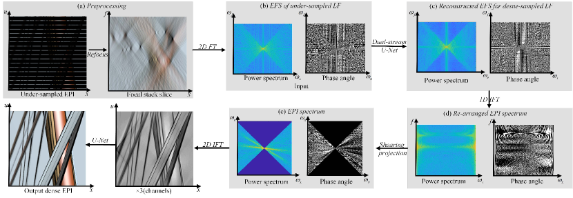
In this paper, we define and explore a novel light field representation, called Epipolar Focus Spectrum (EFS) (in Sec.III). Compared with the classical EPI representation where the slope of the EPI line varies from depth to depth, all contents from the same view will be gathered in a specific line-style zone in the EFS representation, thus the EFS representation is depth independent. This fundamental characteristic provides the basis for pursuing a unified solution to process full disparity contents simultaneously. Apart from this, different from the repeated and overlapped aliasing pattern in the Fourier spectrum of the EPI of an undersampled light field, the EFSs obtained under different angular sampling settings share the same cone-shaped pattern and meet the conjugate symmetry (see Sec.III-C). Therefore, it is more convenient to accurately reconstruct the dense-view light field using the EFS (frequency domain) representation than the EPI (spatial domain) representation. In Sec.IV, we first present an end-to-end convolutional neural network (CNN) to eliminate the aliasing contents in the EFS of an undersampled light field, in which a novel conjugate-symmetric loss is adopted for optimization. Then the generated non-aliasing EFS is projected to construct the EPI spectrum. After applying the inverse Fourier transform (IFT) to obtain the dense-view light field, a U-Net with a perceptual loss is finally utilized to optimize the reconstructed results and eliminate the “trailing image” [28] caused by the integral operation, especially in the marginal view. Experimental results (in Sec.V) verify the effectiveness of the proposed EFS-based dense-view light field reconstruction method.
The main contributions of the work include,
1) A novel depth-invariant representation for light field is defined, named Epipolar Focus Spectrum (EFS), which guarantees the cross-view consistency for full-depth/disparity light field reconstruction.
2) An important characteristic of EFS is explored, that is a same cone-shaped pattern under different angular samplings due to one-to-one mapping from the view to the EFS line. The pattern is determined by the number of views and the disparity gap between neighboring focal planes.
3) An EFS-based learning framework for dense-view light field reconstruction is proposed. Extensive experiments on both synthetic and real light field datasets verify the superiority of the proposed method.
II Related Work
II-A Light field representation
Let represent the distribution of rays in 3D space, where and denote the intersections between the ray with angular/camera and spatial/image planes, respectively [2, 3]. To better model the contents, several representations have been proposed in the literature. In the spatial domain, the sub-aperture image and EPI are the two most common representations. The former emphasizes the spatial information per view. The latter focuses on the disparity among views, where the slope of the EPI lines is associated with the disparity/depth. In the Fourier domain, by exploring the equivalence between the 3D focal stack and a 4D light field, Ng et al. [29] claim the 2D spectrum of a refocused image could be obtained by slicing the corresponding 4D spectrum. Dansereau et al. [30] propose the hyper-cone and hyper-fan representations, which extend the focal range of each focal slice. Le Pendu et al. [31] analyse the sparsity of light field spectrum and propose the Fourier disparity layer (FDL) representation considering the spectrum energy concentrates on several slices.
However, since these representations are highly correlated to the scene depth, the features extracted or learned from the light fields with small disparity range are unsuitable for the light fields with large disparity range, which might leads to wrong inference. In contrast, the proposed EFS is depth-invariant and thus enables an operation or processing covering the whole depth range.
II-B Anti-aliasing of refocusing
Anti-aliasing requires either abundant angular samples or appropriate filters. This problem has been widely studied in both the spatial and frequency domains. In the spatial domain, Levoy and Hanrahan [2] propose a prefilter to reduce the spatial artifacts. Chang et al. [32] propose an anti-aliasing method that compensates the effect of undersampling by utilizing depth information. The technique attempts to interpolate more angular samples within each sampling interval using the depth map. Xiao et al. [33] further analyze the angular aliasing model in the spatial domain. They first detect the aliasing contents and then use lower-frequency terms of the decomposition to remove the angular aliasing at the refocusing stage. In the frequency domain, Isaksen et al. [34] first propose a frequency-planar light field filtering. Chai et al. [19] propose a comprehensive analysis on the trade-off between sampling density and depth resolution. Based on focal stacks and sparse collections of viewpoints, Levin and Durand [35] employ the focal manifold in derivations of 2D deconvolution kernels [31]. After that, Lumsdaine and Georgiev [36] discuss the aliasing in terms of the focal manifold and conclude by rendering wide depth-of-field images. By deriving the frequency domain of support of the light field, Dansereau et al. [30] present a simple, linear single-step filter to achieve volumetric focus effects.
All these methods consider the 3D focal stack as multiple individual slices and remove slice-wise aliasing contents, thus the consistency between neighboring focal slices is not preserved. Different from these methods, the proposed reconstruction method handles aliasing contents of all slices at the same time by treating the 3D focal stack as a whole, so the aliasing could be better removed and meanwhile the consistency is well maintained.
II-C Dense-view reconstruction
As mentioned above, the anti-aliasing operation essentially corresponds to a super-resolution operation in the angular domain [14, 13]. Existing angular super-resolution methods could be mainly divided into two categories.
The first category is based on depth estimation [7, 9, 10, 12]. Wanner et al. [11] reconstruct novel viewpoints by combining input viewpoints and estimated depth information. In order to synthesize novel views from a sparse set of input views, Kalantari et al. [14] propose two convolutional neural networks to estimate the depth and color of each viewpoint sequentially. Srinivasan et al. [12] present a machine learning algorithm that takes a 2D RGB image as input and synthesizes a 4D RGBD light field. Specifically, their pipeline consists of a CNN that estimates scene geometry, and a second CNN that predicts occluded rays and non-Lambertian effects. Subsequently, Srinivasan et al. [17] propose to utilize the MPI representation to synthesize the viewpoint from a narrow baseline stereo pair.
The second category focuses on modeling the consistency of EPI texture [22, 27, 37, 38] or the sparsity of Fourier spectrum [35, 25, 26]. Wu et al. [22] convert the angular domain reconstruction of a 4D light field into a one-dimensional super-resolution of the 2D EPI. Zhu et al. [38] further improve the super-resolution performance on EPI in large disparity areas by introducing a long-short term memory module. Considering the special 2D mesh sampling structure of the 4D light field, Levin et al. [35] utilize the 3D focus stack to complement the spectrum of the 4D light field and achieve the dense reconstruction for sparse light fields. Shi et al. [25] exploit the sparsity of the 4D light field in the continuous Fourier domain and perform the dense light field reconstruction by adopting the sparse Fourier transform. Vagharshakyan et al. [26] utilize a sparse representation of the underlying EPIs in shearlet domain and employ an iterative regularized reconstruction.
Nevertheless, these methods either rely on accurate depth calculations (especially near occlusion boundaries) or are inappropriate for large disparity scenes since the required texture lines or sparse spectrum features are not available. Differently, based on the depth-independent EFS representation, the proposed light field reconstruction method avoids the challenging depth estimation and optimize the contents at various depths with the same strategy.
III The EFS Representation
In this section, we first define the EFS representation for a light field, then introduce its depth-independent characteristics.
III-A Notations
For better understanding the definition of EFS, we first list the notations used in this work, as listed in Tab.I.
Given a 4D light field , denotes its EPI when fixed and and denotes the 2D focal stack integrated by , where and refer to the angular and spatial dimensions respectively. and denote the 1D and 2D Fourier transform respectively (* means specific variable). is the reference view.
In brief, we have the following two equations,
-
1.
.
-
2.
.
| Term | Definition |
|---|---|
| A 4D light field | |
| Angular coordinates | |
| Spatial coordinates | |
| 2D EPI | |
| Sheared EPI at the specific disparity | |
| Disparity range for the shearing process | |
| The number of refocus layers | |
| 1D Fourier transform on the variable * | |
| 2D Fourier transform | |
| Focal stack integrated by | |
| Fourier spectrum of | |
| Slicing and rearranging of | |
| EFS or 2D Fourier spectrum of | |
| Reference view (center view in this work) |
III-B Definition and Construction of EFS
In this section, we first give the definition of EFS and then present two methods for constructing EFS.
Definition. Given a 2D EPI , the EFS representation is defined as the 1D Fourier transform along the -axis of the rearranged EPI Fourier spectrum slices. In detail, a slice operation is firstly applied on to construct ,
| (1) |
where the disparity takes value in the interval . Then the EFS is obtained by the 1D Fourier transform of along the -axis,
| (2) |
According to Eq.1, contains all spectrum contents of the EPI when and . In other words, the EFS could represent the EPI losslessly in this case.
.
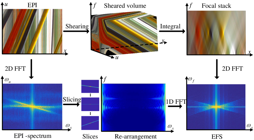
Construction. From the above definition, the EFS could be constructed based on the Fourier slice of , as shown in the bottom branch in Fig.1.
Alternatively, the EFS could also be obtained in the spatial domain according to the Fourier slice photography theorem [29]. Firstly, denotes the sheared EPI at a specific disparity ,
| (3) |
After that, once the sheared EPI with an arbitrary disparity is integrated over all the views, the focal stack is formed,
| (4) |
Then by performing the 2D Fourier transform on the focal stack, we can obtain the corresponding EFS representation,
| (5) |
Noting that, the lossless EFS could only be constructed in two cases, i.e., or the infinite aperture size [35]. However, since these conditions are practically impossible to achieve, the EFS is actually a lossy representation in practice. To minimize the effects of the missing spectrum in , it is suggested to set and as the minimum and maximum disparities of the scene respectively. A detailed analysis on this issue will be given in Sec.V-C .
III-C Characteristics of EFS
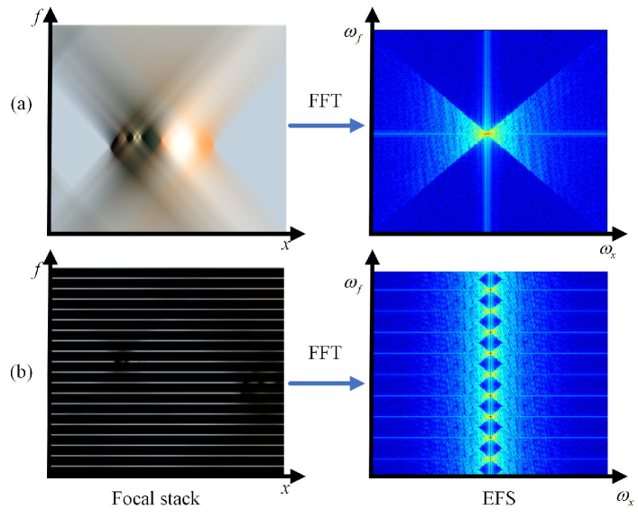
According to the second construction method, the EFS is equal to the Fourier spectrum of the focal stack. In this section, we first analyze the characteristics of the focal stack under different values of , then discuss the attributes of EFS in the Fourier domain.
III-C1 Defocus and Aliasing in the Focal Stack
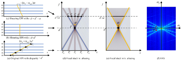
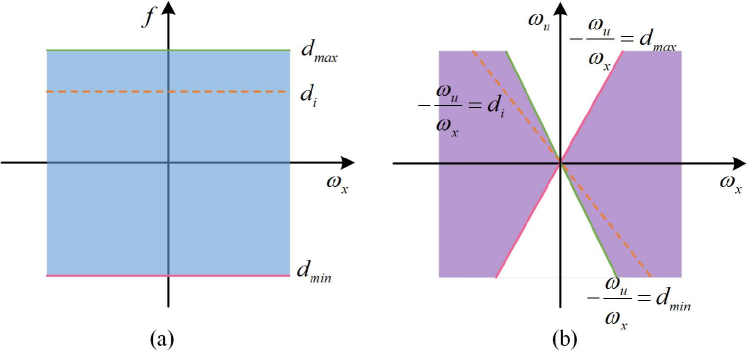
Fig.2 (a) shows an EPI line for a pixel with disparity . The EPI is sheared with (in Fig.2 (b)) according to Eq.3. Since the EPI line is now perpendicular to the -axis, there is no aliasing or defocus blur at in the refocused image, as shown in Fig.2 (d) and (e). Then the original EPI is sheared with (see Fig.2 (c)). It is noticed that the EPI line is not perpendicular to -axis anymore and the aliasing or defocus blur appears again in the focal stack, as illustrated in the layer in Fig.2 (d) and (e) respectively. The radius of the aliasing or defocus blur increases with the increasing of and a triangle is formed in the focal stack slice. Noting that, since the baseline between neighboring views is scaled by when inserting views, the defocus diameter in Fig.2(e) is equal to the aliasing distance in Fig.2(d). The apex angle in Fig.2(e) does NOT change (the same cone-shaped pattern still exists, as shown in Fig.2(e)).
Without loss of generality, only the horizontal angular sampling is discussed here. Suppose that the light field has views, the apex angle of the triangle has two forms,
| (6) |
where is the disparity gap between neighboring focal planes when constructing the focal stack as shown in Fig.3.
The diameter of the defocus blur (or aliasing), i.e., the interval between and in Fig.2 (d), can be calculated by
| (7) |
Note that, the aliasing only occurs when holds. Furthermore, for textured areas, the aliasing always exists in the refocused image as long as the sheared parameter is large enough.
Revisiting Eq.3, it is found that the aliased pixels , , come from the views , , respectively. The slope of each aliasing line in Fig.2(d) can be computed by
| (8) |
-
a)
The shape of the defocus blur or aliasing line is determined by both the disparity gap and the view index, and it is independent of the scene depth.
-
b)
All aliasing lines from the same view have the same slope.
III-C2 Views sampling in the EFS
According to the second property, given a focal stack formed from a -view light field, there are frequency lines in the EFS according to the property of the Fourier transform [39]111Fourier transform tells the energy of all lines with the same slope in the spatial domain concentrates on a perpendicular line passing through the origin.. Each line corresponds to a specified view, and more views lead to more lines. Consequently, the EFS has the following properties,
-
a)
The shape of the EFS pattern is determined by both the refocus parameter and the number of views, and it is independent of the scene depth.
-
b)
According to the property of the Fourier transform [40], the EFS is conjugate symmetric.
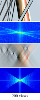
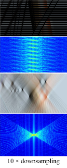
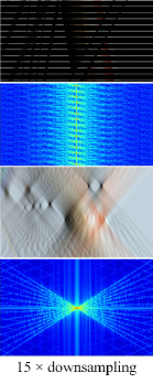
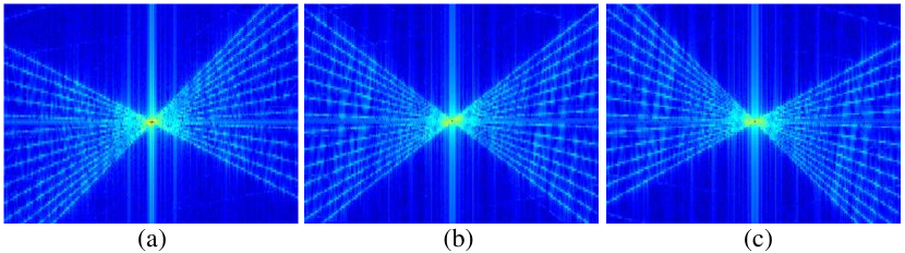
Fig.4 provides several examples of the EPI, EPI spectrum, focal stack and EFS under different sampling rates. Taking a closer look at the EPI spectrum (the 2nd row) and the EFS (the last row) in Fig.4, it is worth noting that with a reduction of the view count, more repeating patterns appear in the EPI spectrum, while the structure of the EFS distribution almost remains unchanged. Additionally, there is a one-to-one correspondence between the line in the EFS and the view index when is fixed. As shown in Fig.4(c), 14 views in the EPI correspond to 14 lines in the EFS.
III-D Sampling analysis of EFS
There are mainly two reasons for aliasing in the EFS, one is sparse angular sampling (Fig.4(b)(c)), the other is insufficient refocus layers (Fig.5). Since the EFS structure basically remains in the first case, here we focus on the second case caused by insufficient refocus layers, and analyze the lower bound of focal stack layers required for non-aliasing EFS recovery.
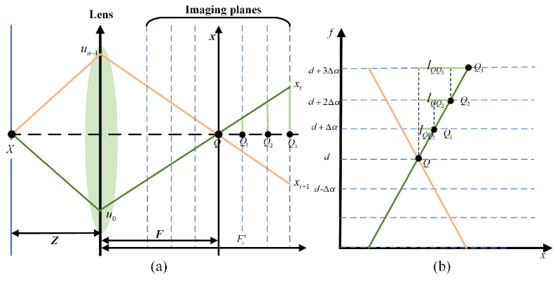
As shown in Fig.5, when the refocus range of the focal stack is equal to the depth range for all the objects in the scene, aliasing appears when the disparity gap between neighboring focal layers increases. To eliminate aliasing, all lines formed from different views in the focal stack ought to be continuous instead of being discrete, i.e., . All the inequalities for the middle views hold if the inequalities for two marginal views hold. In other words, the disparity gap should meet the following inequality,
| (9) |
The refocus range is set according to the scene depth range ,
| (10) |
where is the focal length and is the baseline. Thus, the number of refocus layers in the focal stack is calculated by
| (11) |
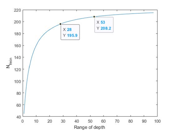
When the depth is discontinuous, it is essential to take the scene distribution into consideration. The minimum number of focal layers is estimated as
| (13) |
where denotes the scene distribution function, determined by the depth , occlusion and texture .
In summary, the lower bound of focal stack layers is determined by the relative depth variation (), scene distribution and the baseline of the synthetic aperture optical system. Fig.6 illustrates an example of choosing , where , (a continuous depth distribution), , . The depth takes value in the interval . Particularly, the black line curve shows the varying trend of with . Refer to Sec.V-C for more experimental analysis.
IV EFS-based Dense-view Reconstruction
Insufficient angular sampling causes aliasing in the focal stack, thus reconstructing a dense-view light field is equivalent to restoring a complete EFS corresponding to the non-aliasing light field/focal stack. As analyzed in Sec.III-C, we can complement the non-aliased EFS by learning to recover the spectrum lines corresponding to missing viewpoints. Therefore, the light field reconstruction task is formulated as an EFS completion problem in this work. The pipeline of the proposed dense-view light field reconstruction is shown in Fig.7.
IV-A EFS reconstruction
Specifically, We first perform shearing on an undersampled EPI to get the focal stack by Eq.4, then apply the Fourier transform on the aliased focal stack to get the aliased EFS (Eq.5). Subsequently, a CNN parameterized by is proposed to complete the spectrum in the aliased . The parameter is optimized by
| (14) |
The loss function is,
| (15) |
where the scalar is set to 1.5 for balancing the contributions of two loss terms. The second term constrains the conjugate symmetry of the reconstructed EFS,
| (16) |
where refers to the norm of a complex number and indicates the standard conjugate operation. and are the number of refocus layers and the width of sub-aperture image respectively.
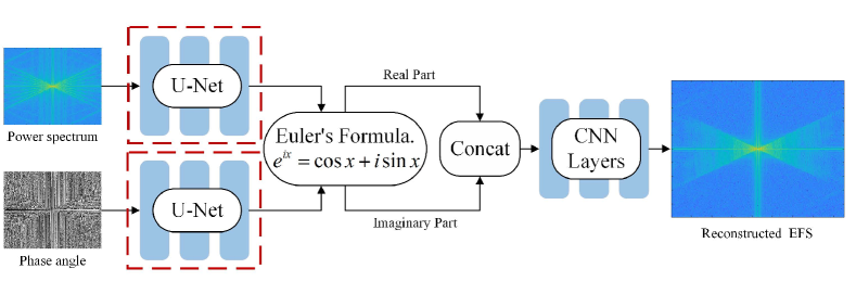
As shown in Fig.8, a novel dual-stream U-Net is designed to deal with complex number inputs. The power spectrum and phase angle are firstly fed into two sub-networks respectively. Then the features are combined using the Euler’s formula to obtain the real and imaginary parts, which are concatenated and passed into several CNN layers for optimization. The detail of dual-stream U-Net is shown in the supplemental materials.
IV-B EPI reconstruction
The Fourier Slice Imaging Theorem [29] tells a 2D slice through the origin of a 4D light field spectrum corresponds to a refocused image at a certain depth in the frequency domain. Based on this, we first apply the 1D inverse Fourier transform (IFT) of EFS along the -axis,
| (17) |
The projection relationship between and can be obtained via Eq.1. Thus the Fourier spectrum of the reconstructed EPI could be calculated by performing a reverse projection,
| (18) |
Fig.9 shows the diagram of this reverse projection. Due to the limitation of disparity range, only the spectrum labeled as purple of Fig.9(b) can be reconstructed with this operation.
The next step is to apply the 2D IFT to get from . Since the interpolation operation is used during the focal stack construction, the “tailing” effects appear after the inverse Fourier slice operation, especially for the marginal viewpoints which are far away from the reference view. Hence we use the U-Net with a perceptual loss to optimize the reconstructed EPIs ,
| (19) |
where represents the ground truth EPI.
The loss function for optimization is defined as follow,
| (20) |
where is the Mean Absolute Error loss, is the Structural Similarity loss [41], and is the perceptual loss[42] which is based on the VGG19 network trained on ImageNet. The scalars are set to 3 and 5 for balancing the effects of different loss terms. The detailed structure of this network is illustrated in the supplementary materials.
The complete dense-view light field reconstruction algorithm is given in Algorithm 1. represents the height of the sub-aperture image.
V Evaluations
To evaluate our proposed EFS-based dense-view light field reconstruction method, we conduct experiments on both synthetic and real light field datasets. The real light field datasets are captured by both the camera array and the plenoptic camera (Lytro Illum [43]). We mainly compare our approach with two state-of-the-art learning-based methods, Wu et al. [22] (without explicit depth estimation) and LLFF [44] (MPI-based). Note that LLFF [44] is retrained on our training date using the released training code for fair comparison. For Wu et al. [22] without the original code being released, we just use the trained model provided by the authors.
To empirically validate the robustness of the proposed method, we perform evaluations under different sampling patterns. The quantitative evaluations are performed by measuring the average PSNR and SSIM metrics over the synthetic views of the luminance channel. We also analyse the spectrum energy losses for EFS reconstruction and EPI reconstruction respectively.
V-A Datasets and Implementation Details
In the training process, both the synthetic and real light fields are used. For the synthetic data, 12 light fields containing complex textured structures are rendered using the automatic light field generator [38, 45], of which 7 are for training and 5 for testing. Real light fields are taken from the high-resolution light field dataset provided by Guo et al. [37], of which 20 are for training and 6 for testing. In order to show the relationship between viewpoints and EFS lines, we utilize the first 200 viewpoints for experiments. Additionally, the light fields from the Disney [46] dataset are used to verify the performance of the proposed method on unseen scenes captured by a camera array. Tab.II displays the parameters of all the datasets. In the dense-view light fields, the disparity between two adjacent views for most scenes is less than one pixel, while in several scenarios, the disparity reaches two pixels.
| Dataset | Angular Res. | Spatial Res. |
|---|---|---|
| Syn. LFs | ||
| Real LFs [37] | ||
| Couch [46] | ||
| Church [46] | ||
| Bike[46] | ||
| Statue[46] |
At present, only the disparity along one single direction is concerned so that the 2D EPIs can represent the input light field. The details of several light fields under 10 and 15 downsampling scales is shown in the supplementary materials. For each light field in the experiment, by considering the disparity and the scene distribution, the EFS is constructed by performing the refocus operation for 200 times () where . The range of scene disparity determines the range of refocusing operation . For details regarding the disparity, refer to our datasets and codes released later.
V-B Spectrum Domain
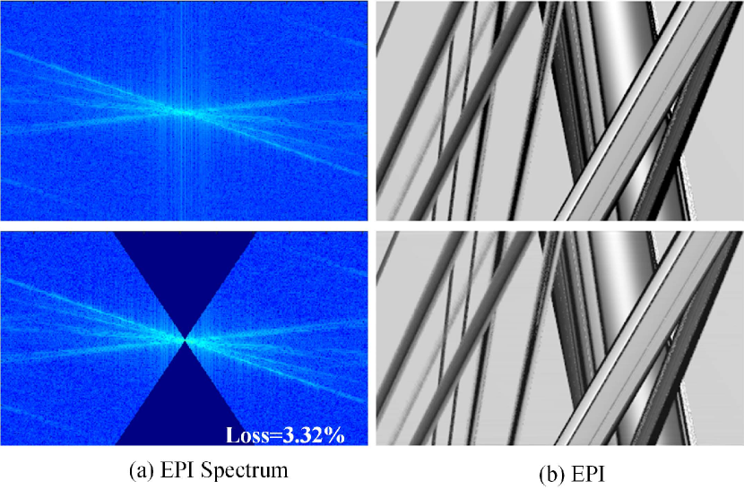
EPI spectrum loss analysis. In our experiments, the disparity range is also the focal stack range. With the infinite aperture assumption, the spectrum energy could be regarded as zero for other focus layers beyond the constructed focal stack[35]. However, since the infinite aperture camera is currently not available, the EFS representation for a light field has a certain loss. Fig.10 shows the difference between the whole dense-view EPI spectrum and the EPI spectrum within a certain disparity range obtained from the EFS. Although partial contents are missing in the latter case (about 3.32), the structural information on the EPI can still be reconstructed.
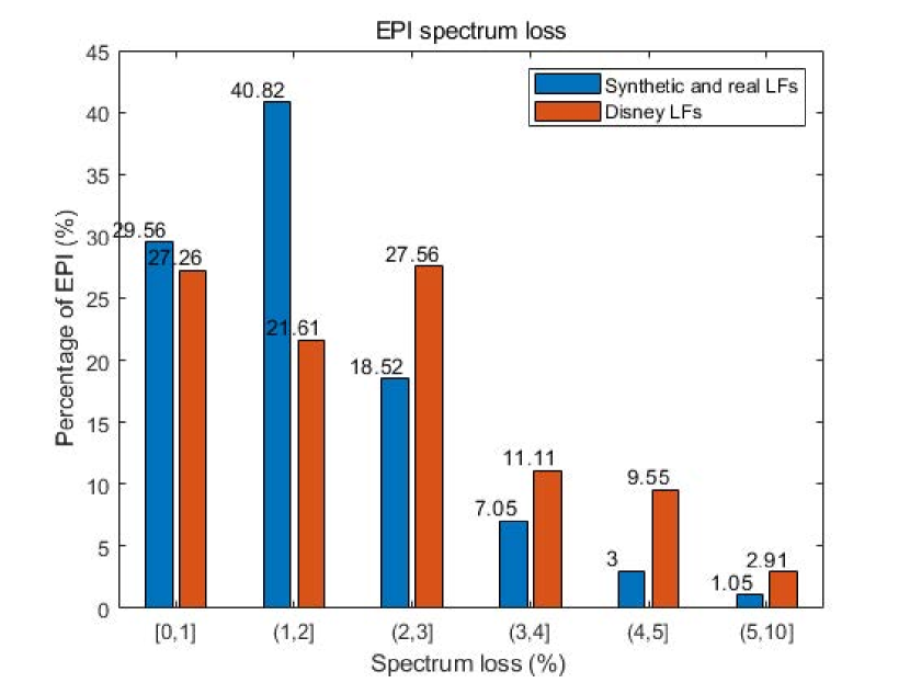
To evaluate the upper bound of the EPI spectrum loss in a dense-view light field, we have counted the spectral energy loss over 10,000 EPIs which are reconstructed from the EFS containing all the scene depth ranges for several light fields and summarized the results in Fig.11. In these EPI spectra, the maximum loss is 9.03, the minimum loss is 0.31, and the average loss is 1.94. It can be seen that the EPI spectrum loss generally has a sparse ( 5) distribution. In addition, the distribution of the loss on Disney LFs[46] is flatter and more spread out than that on synthetic[45] and real LFs[37]. We attribute this to: 1) the background texture of Synthetic LFs is relatively simple, while the texture of Disney LFs is more complex, 2) the scene depth of Synthetic data is primarily concentrated within a limited interval, while the depth distribution of Disney LFs is more divergent.
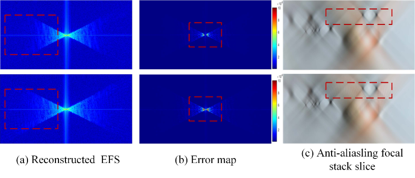
EFS reconstruction loss analysis. We try to analyze the loss in the EFS reconstruction. Some results are displayed in Fig.12, which consists of reconstructed EFS, the error map, and corresponding anti-aliasing focal stack.
V-C Parameter analysis
We empirically validate the influences of the range of refocus operation and the EFS sampling on the reconstructed EPI by performing the following parameter analysis. In these experiments, we use our synthetic light fields with 15 downsampling.
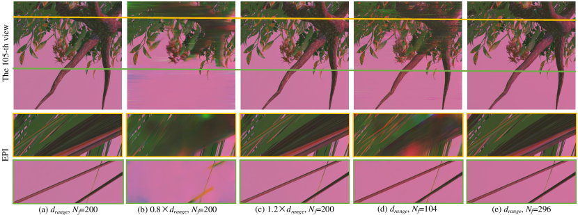
The range of refocus operation. The refocus range is set to 0.8, and 1.2, respectively. As mentioned in Sec.V-B, with 15 downsampling of the original light field, is the scene disparity range (). Fig.13 (a)(b)(c) show the qualitative comparisons with different refocus ranges on the tree root dataset. Quantitative analysis, in terms of average PSNR and SSIM, is summarized in the 2nd, 3rd and 4th rows of Tab.IV. As shown in Fig.13 (b), partial tree root has not been reconstructed. The scene structure can not be reconstructed completely when the range of refocus operation is too narrow.
The number of EFS layers . The number of refocus layers is set to 104, 200 and 296, respectively. Fig.13 (a)(d)(e) show the qualitative comparisons with different numbers of EFS layers. The 2nd, 5th, and 6th rows of Tab.IV show the quantitative comparison on reconstructed light fields. It is noticed that insufficient focal layers, of which the count is smaller than the minimum focal layer count (see Sec.III-D), i.e., =104, will cause performance degradation ( in terms of PSNR and SSIM respectively). In this case, aliasing appears in the focal stack, which leads to over-smooth textures in Fig.13(d). In addition, when is increased from 200 to 296, only a slight improvement in the performance is reported ( ). Hence once the number of EFS layers meets the minimum sampling rate requirement, continuously increasing EFS layers would not bring obvious improvements in the performance.
| Refocus range | # EFSs | PSNR | SSIM |
|---|---|---|---|
| 200 | 35.05 | 0.865 | |
| 200 | 37.54 | 0.952 | |
| 200 | 37.96 | 0.959 | |
| 104 | 32.92 | 0.823 | |
| 296 | 37.98 | 0.961 |
V-D Comparisons with SOTAs
We compare our method against Wu et al. [22] and LLFF [44]. Tab.V shows the average PSNR/SSIM/LPIPS[47] measurements with different downsampling rates on both synthetic and real light fields. Qualitative comparisons between different methods on several test scenes under 15 downsampling rate are shown in Fig.14, Fig.15 and Fig.16 respectively.
V-D1 Synthetic light field datasets
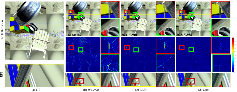
We evaluate the proposed approach using our synthetic light field datasets under 10 and 15 downsampling rates. Qualitative results under 15 downsampling (maximum disparity up to 8px) are shown in Fig.14.
As shown in Fig.14(b), ghosting artifacts are visible around the boundary region in the reconstruction result by Wu et al. [22], which are caused by the limited receptive field of their network. Also, the Gaussian convolution kernel is only effective for small disparity. The MPI-based LLFF [44] tends to assign high opacity to incorrect layer for the region with ambiguous/repetitive texture or moving content between input images, which will cause floating or blurred patches around the boundary region (see the boundary region of the pot in Fig.14(c)). In comparison, the proposed EFS-based reconstruction method produces more clear boundaries (as shown in Fig.14(d)).
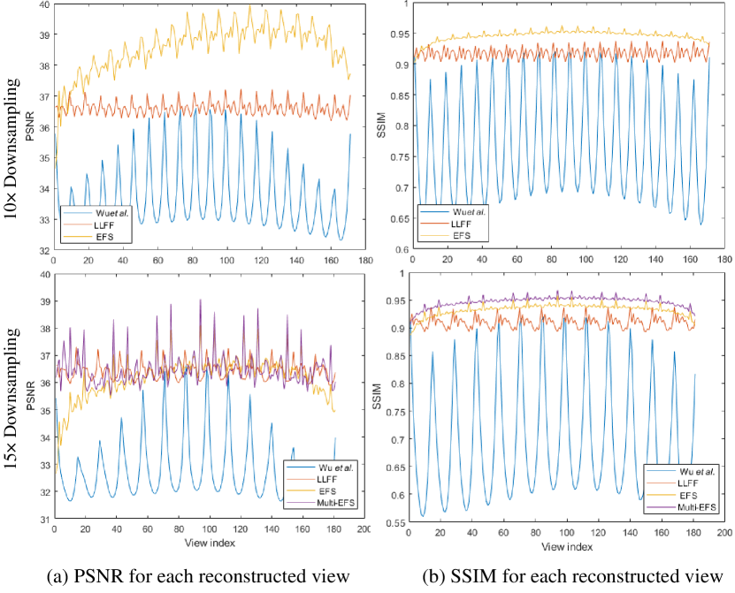
Fig.17 shows the PSNR and SSIM measurements for each reconstructed view on the synthetic light field under 10 and 15 downsampling rates. Due to the shearing process used in our method (Eq.(3)), the more marginal views there are, the more image information will be sheared out of the image. Thus the reconstruction results are not satisfactory on these marginal views. Still, the overall performance of our method is better than the SOTAs, especially for larger disparity scenarios. The 3rd and 4th columns of Tab.V list the quantitative measurements on synthetic light fields under different downsampling rates, which further validates the superiority of the proposed method.
V-D2 Real light fields captured with a plenoptic camera
We also evaluate the proposed approach using the Lytro light field dataset [37], which contains massive static scenes in the real world, such as bicycles, toys, and plants. These scenes are challenging in terms of abundant colors and complicated occlusions.
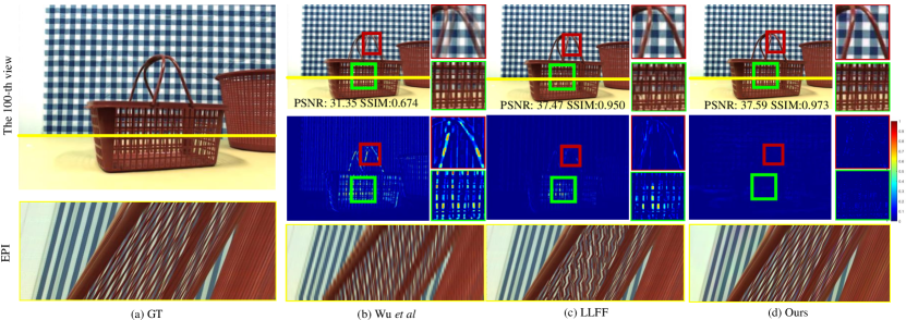
Fig.15 shows the reconstruction results of “basket” under 15 downsampling. There exist many thin structures in the scene, such as the basket handle. The texture on such a thin structure changes very fast, which results in difficulties for reconstruction. We can see that severe ghosting artifacts occur around the basket handle in the results by Wu et al. [22] and reconstructed views are inconsistent (Fig.15(b)). Similarly, a fuzzy phenomenon appears in the results by LLFF [44] on the handle part. By reconstructing the dense light field in the frequency domain, our method is less sensitive to the spatial contents, and thus capable of producing high-quality and consistent view reconstruction.
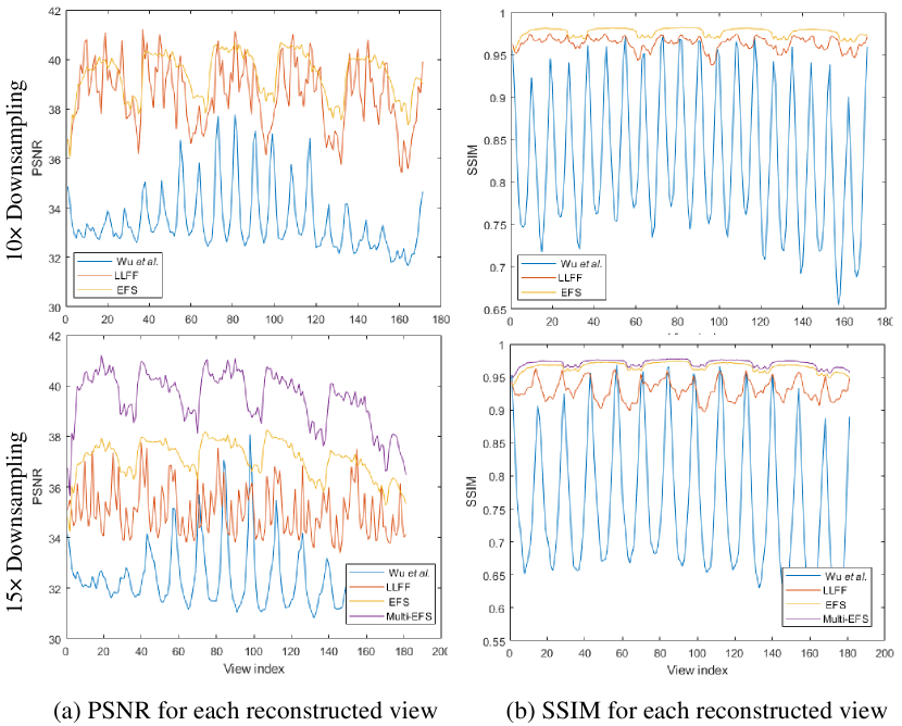
Fig.18 shows the PSNR and SSIM measurements for each reconstructed view of Fig.15 under 10 and 15 downsampling. As for the high complexity of the scene, over 95 view reconstruction results by our method are better than SOAT methods. Quantitative comparisons in terms of PSNR, SSIM, and LPIPS are listed in the 5th and 6th columns of Tab.V.
V-D3 Real light fields captured with a camera array

In order to verify the effectiveness of our method under wide baseline and large disparity conditions, we further evaluate the proposed approach using the Disney light fields [46] which are captured by a camera array.
Fig.16 shows the reconstruction results on the statue scene under 10 downsampling (maximum disparity up to 15px). Due to the limited receptive field of the networks, the results by Wu et al. [22] show serious aliasing effects on all the foreground objects (Fig.16(b)). Due to the memory limitation, there is a trade-off between the image resolution and the layers of MPIs utilized by LLFF[44], which leads to performance degradation for large disparity areas with high-resolution input. Also severe artifacts appears in the regions with repetitive patterns, large disparity and occlusions, as shown in the zoom-in rectangles in Fig.16(c). This is a common failure mode for the methods which rely on texture matching cues to infer depth. In contrast, thanks to the depth-independent characteristic, our proposed method shows better performance under large disparities. Furthermore, it is noticed that the proposed method maintains better view consistency compared with other methods. Quantitative results on several Disney light fields are shown in the last four columns of Tab.V.
In addition, by comparing the results of our method in Tab.V with Tab.III, we find that the average EFS spectral energy loss has a significant influence on PSNR while having much less effect on SSIM. This demonstrates the robustness of the proposed reconstruction method, considering the fact that human eyes are more sensitive to changes of the structure information (SSIM) than individual pixel values (PSNR) [48].
| Syn. LFs | Real LFs [37] | Bike [46] | Church [46] | Couch [46] | Statue [46] | ||||
|---|---|---|---|---|---|---|---|---|---|
| Wu [49] | PSNR | 35.48 | 34.77 | 36.14 | 34.92 | 31.13 | 32.64 | 32.01 | 32.63 |
| SSIM | 0.851 | 0.813 | 0.877 | 0.825 | 0.708 | 0.721 | 0.724 | 0.698 | |
| LPIPS | 0.060 | 0.093 | 0.050 | 0.078 | 0.110 | 0.080 | 0.113 | 0.098 | |
| LLFF [44] | PSNR | 37.29 | 36.46 | 39.74 | 37.02 | 35.51 | 38.85 | 37.25 | 38.53 |
| SSIM | 0.941 | 0.922 | 0.964 | 0.925 | 0.875 | 0.962 | 0.916 | 0.956 | |
| LPIPS | 0.059 | 0.089 | 0.039 | 0.079 | 0.082 | 0.051 | 0.084 | 0.049 | |
| Ours | PSNR | 39.36 | 37.54 | 40.18 | 37.74 | 36.77 | 37.95 | 43.05 | 40.82 |
| SSIM | 0.963 | 0.952 | 0.948 | 0.938 | 0.939 | 0.964 | 0.928 | 0.959 | |
| LPIPS | 0.056 | 0.088 | 0.043 | 0.072 | 0.085 | 0.060 | 0.079 | 0.041 | |
V-E Multi-reference-view results
As shown in Fig.17 and Fig.18, the reconstruction performance for some edge views by our method (only one center reference) has been slightly below than that of the SOTAs. This is because the center reference view does not contain enough side-view information when the baseline is large. In this section, we use multi-reference views to build Multi-EFSs to provide more information for marginal view reconstruction.
Fig.19 show the reconstructed Multi-EFSs, which is built using the 30th view ahead of the center view (), the center reference () and the 30th view behind the center view(). The bottom row of Fig.17 and Fig.18 show the PSNR and SSIM measurements for each reconstructed view of Fig.14 and Fig.15. It can be seen that the Multi-EFSs significantly improve the overall performance of our EFS-based method, especially for edge views.
V-F Full parallax results
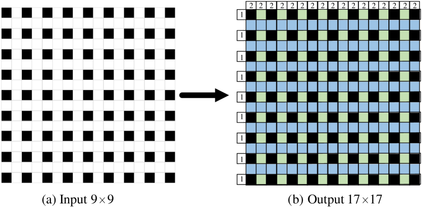
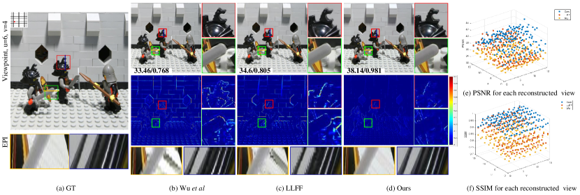
The sequential solution for full parallax is reconstructing the views containing vertical disparities after all the views containing horizontal disparities have been reconstructed, which is illustrated using an array of full parallax reconstructed from the input views (marked in black) in Fig.20. As shown in Fig.20(b), the views marked in green are firstly reconstructed in the horizontal parallax reconstruction step, and the views marked in blue are later reconstructed in the vertical parallax reconstruction step. We validate this solution on the Lego dataset[50] and show the qualitative and quantitative results in Fig.21.
| Wu et al. [22] | LLFF [44] | Ours | |
|---|---|---|---|
| PSNR | 36.29 | 37.71 | 39.02 |
| SSIM | 0.862 | 0.895 | 0.965 |
Due to the lager disparity of the Lego dataset, there exist obvious artifacts near boundary regions and discontinuous EPIs in both the results by Wu et al. [22] and LLFF [44]. Additionally, LLFF [44] usually requires a large dataset for model training, while our method is capable of learning the relationship between viewpoints and spectrum lines in the frequency domain from a relatively small training dataset. The experimental results show that our proposed method can generate clear edges and preserve cross-view consistency. Tab.VI shows the average PSNR and SSIM on the Lego dataset.
V-G Limitation
At present, the energy loss of the spectrum still exists, which may lead to unevenly colored reconstructed views. A possible solution to deal with this issue could be the space-frequency combined method, or adding a visual channel to compensate for the energy loss in the frequency domain. In addition, although the proposed method outperforms the SOTA methods on both view reconstruction quality and cross-view consistency preservation, the shearing operation may cause a moderate decline in the reconstruction performance for the marginal views (Sec.V-D). This could be addressed by introducing more reference views during the construction of the focal stack to provide more required information on the scene.
VI Conclusions
We present a novel EFS representation for light fields, of which the advantages include: (1) it is depth-independent, (2) its structure remains basically unchanged under different angular sampling rates, and (3) each EFS-line corresponds to one view in the light field. Thanks to these characteristics, we further propose an EFS-based method for reconstructing a dense-view light field from an undersampled light field, by reconstructing EFS-lines in the spectrum domain without using scene depth or any spatial information. The proposed method exhibits superior performance under many challenging conditions, such as large disparities and complex occlusions, and maintains the cross-view consistency.
References
- [1] E. H. Adelson and J. R. Bergen, “The plenoptic function and the elements of early vision.” Computational Models of Visual Processing, vol. 1, no. 2, pp. 3–20, 1991.
- [2] M. Levoy and P. Hanrahan, “Light field rendering,” in ACM SIGGRAPH. ACM, 1996, pp. 31–42.
- [3] S. J. Gortler, R. Grzeszczuk, R. Szeliski, and M. F. Cohen, “The lumigraph,” in ACM SIGGRAPH, 1996, pp. 43–54.
- [4] C. Richardt, P. Hedman, R. S. Overbeck, B. Cabral, R. Konrad, and S. Sullivan, “Capture4VR: From VR photography to VR video,” in SIGGRAPH Courses, 2019. [Online]. Available: https://richardt.name/Capture4VR/
- [5] T. Georgiev, K. C. Zheng, B. Curless, D. Salesin, S. K. Nayar, and C. Intwala, “Spatio-angular resolution tradeoffs in integral photography,” Rendering Techniques, vol. 2006, no. 263-272, p. 21, 2006.
- [6] M. Eisemann, B. De Decker, M. Magnor, P. Bekaert, E. De Aguiar, N. Ahmed, C. Theobalt, and A. Sellent, “Floating textures,” Wiley CGF, vol. 27, no. 2, pp. 409–418, 2008.
- [7] M. Goesele, J. Ackermann, S. Fuhrmann, C. Haubold, R. Klowsky, D. Steedly, and R. Szeliski, “Ambient point clouds for view interpolation,” ACM TOG, vol. 29, no. 4, pp. 95:1–95:6, 2010.
- [8] G. Chaurasia, O. Sorkine, and G. Drettakis, “Silhouette-aware warping for image-based rendering,” Wiley CGF, vol. 30, no. 4, pp. 1223–1232, 2011.
- [9] G. Chaurasia, S. Duchene, O. Sorkine-Hornung, and G. Drettakis, “Depth synthesis and local warps for plausible image-based navigation,” ACM TOG, vol. 32, no. 3, pp. 30:1–30:12, 2013.
- [10] E. Penner and L. Zhang, “Soft 3D reconstruction for view synthesis,” ACM TOG, vol. 36, no. 6, pp. 235:1–235:11, 2017.
- [11] S. Wanner and B. Goldluecke, “Variational light field analysis for disparity estimation and super-resolution,” IEEE T-PAMI, vol. 36, no. 3, pp. 606–619, 2014.
- [12] P. P. Srinivasan, T. Wang, A. Sreelal, R. Ramamoorthi, and R. Ng, “Learning to synthesize a 4D RGBD light field from a single image,” in IEEE ICCV, 2017, pp. 2262–2270.
- [13] T.-C. Wang, J.-Y. Zhu, N. K. Kalantari, A. A. Efros, and R. Ramamoorthi, “Light field video capture using a learning-based hybrid imaging system,” ACM TOG, vol. 36, no. 4, pp. 133:1–133:13, 2017.
- [14] N. K. Kalantari, T.-C. Wang, and R. Ramamoorthi, “Learning-based view synthesis for light field cameras,” ACM TOG, vol. 35, no. 6, pp. 193:1–193:10, 2016.
- [15] T. Zhou, R. Tucker, J. Flynn, G. Fyffe, and N. Snavely, “Stereo magnification: Learning view synthesis using multiplane images,” ACM TOG, vol. 37, no. 4, pp. 65:1–65:12, 2018.
- [16] J. Flynn, M. Broxton, P. Debevec, M. DuVall, G. Fyffe, R. Overbeck, N. Snavely, and R. Tucker, “Deepview: View synthesis with learned gradient descent,” in IEEE CVPR. IEEE, 2019, pp. 2367–2376.
- [17] P. P. Srinivasan, R. Tucker, J. T. Barron, R. Ramamoorthi, R. Ng, and N. Snavely, “Pushing the boundaries of view extrapolation with multiplane images,” in IEEE CVPR, 2019, pp. 175–184.
- [18] B. Mildenhall, P. P. Srinivasan, R. Ortiz-Cayon, N. K. Kalantari, R. Ramamoorthi, R. Ng, and A. Kar, “Local light field fusion: Practical view synthesis with prescriptive sampling guidelines,” ACM TOG, 2019.
- [19] J.-X. Chai, X. Tong, S.-C. Chan, and H.-Y. Shum, “Plenoptic sampling,” in ACM SIGGRAPH. ACM, 2000, pp. 307–318.
- [20] C. Zhang and T. Chen, “Generalized plenoptic sampling,” Carnegie Mellon University, Pittsburgh, PA 15213, Technical Report AMP01-06, September 2001.
- [21] Y. Wang, F. Liu, Z. Wang, G. Hou, Z. Sun, and T. Tan, “End-to-end view synthesis for light field imaging with pseudo 4DCNN,” in Springer ECCV, 2018, pp. 340–355.
- [22] G. Wu, Y. Liu, L. Fang, Q. Dai, and T. Chai, “Light field reconstruction using convolutional network on epi and extended applications,” IEEE T-PAMI, vol. 41, no. 7, pp. 1681–1694, 2019.
- [23] H. W. F. Yeung, J. Hou, J. Chen, Y. Y. Chung, and X. Chen, “Fast light field reconstruction with deep coarse-to-fine modelling of spatial-angular clues,” in Springer ECCV, 2018, pp. 137–152.
- [24] G. Wu, Y. Liu, Q. Dai, and T. Chai, “Learning sheared epi structure for light field reconstruction,” IEEE T-IP, vol. 28, no. 7, pp. 3261–3273, 2019.
- [25] L. Shi, H. Hassanieh, A. Davis, D. Katabi, and F. Durand, “Light field reconstruction using sparsity in the continuous fourier domain,” ACM TOG, vol. 34, no. 1, pp. 12:1–12:13, 2014.
- [26] S. Vagharshakyan, R. Bregovic, and A. Gotchev, “Light field reconstruction using shearlet transform,” IEEE T-PAMI, vol. 40, no. 1, pp. 133–147, 2018.
- [27] Y. Yoon, H.-G. Jeon, D. Yoo, J.-Y. Lee, and I. So Kweon, “Learning a deep convolutional network for light-field image super-resolution,” in IEEE ICCV Workshops, 2015, pp. 24–32.
- [28] S. Inamori and S. Yamauchi, “A method of noise reduction on image processing,” IEEE Transactions on Consumer Electronics, vol. 39, no. 4, pp. 801–805, 1993.
- [29] R. Ng, “Fourier slice photography,” in ACM TOG, vol. 24, no. 3. ACM, 2005, pp. 735–744.
- [30] D. G. Dansereau, O. Pizarro, and S. B. Williams, “Linear volumetric focus for light field cameras,” ACM TOG, vol. 34, no. 2, p. 15, 2015.
- [31] M. Le Pendu, C. Guillemot, and A. Smolic, “A fourier disparity layer representation for light fields,” IEEE T-IP, vol. 28, no. 11, pp. 5740–5753, Nov 2019.
- [32] A. Chang, T. Sung, K. Shih, and H. H. Chen, “Anti-aliasing for light field rendering,” in IEEE ICME, 2014, pp. 1–6.
- [33] Z. Xiao, Q. Wang, G. Zhou, and J. Yu, “Aliasing detection and reduction scheme on angularly undersampled light fields,” IEEE T-IP, vol. 26, no. 5, pp. 2103–2115, 2017.
- [34] A. Isaksen, L. McMillan, and S. J. Gortler, “Dynamically reparameterized light fields,” in ACM SIGGRAPH. ACM, 2000, pp. 297–306.
- [35] A. Levin and F. Durand, “Linear view synthesis using a dimensionality gap light field prior,” in IEEE CVPR, 2010, pp. 1831–1838.
- [36] A. Lumsdaine, T. Georgiev et al., “Full resolution lightfield rendering,” Indiana University and Adobe Systems, Tech. Rep, vol. 91, p. 92, 2008.
- [37] M. Guo, H. Zhu, G. Zhou, and Q. Wang, “Dense light field reconstruction from sparse sampling using residual network,” in Springer ACCV, 2018, pp. 1–14.
- [38] H. Zhu, M. Guo, H. Li, Q. Wang, and A. Robles-Kelly, “Revisiting spatio-angular trade-off in light field cameras and extended applications in super-resolution,” IEEE T-VCG, vol. 27, no. 6, pp. 3019–3033, 2021.
- [39] J. Bigun, “Optimal orientation detection of linear symmetry,” in IEEE ICCV, 1987, pp. 433–438.
- [40] R. C. Gonzales and R. E. Woods, “Digital image processing,” 2002.
- [41] Z. Wang, A. C. Bovik, H. R. Sheikh, and E. P. Simoncelli, “Image quality assessment: from error visibility to structural similarity,” IEEE TIP, vol. 13, no. 4, pp. 600–612, 2004.
- [42] J. Johnson, A. Alahi, and L. Fei-Fei, “Perceptual losses for real-time style transfer and super-resolution,” in Springer ECCV. Cham: Springer International Publishing, 2016, pp. 694–711.
- [43] Lytro, “Lytro redefines photography with light field cameras,” http://www.lytro.com, 2011.
- [44] B. Mildenhall, P. P. Srinivasan, R. Ortiz-Cayon, N. K. Kalantari, R. Ramamoorthi, R. Ng, and A. Kar, “Local light field fusion: Practical view synthesis with prescriptive sampling guidelines,” ACM TOG, vol. 38, no. 4, pp. 1–14, 2019.
- [45] POV-ray, http://www.povray.org/.
- [46] C. Kim, H. Zimmer, Y. Pritch, A. Sorkine-Hornung, and M. H. Gross, “Scene reconstruction from high spatio-angular resolution light fields,” ACM TOG, vol. 32, no. 4, pp. 73:1–73:12, 2013.
- [47] R. Zhang, P. Isola, A. A. Efros, E. Shechtman, and O. Wang, “The unreasonable effectiveness of deep features as a perceptual metric,” in IEEE CVPR, 2018, pp. 586–595.
- [48] Z Wang, A. C. Bovik, H. R. Sheikh, and E. P. Simoncelli, “Image quality assessment: from error visibility to structural similarity,” IEEE TIP, vol. 13, no. 4, pp. 600–612, 2004.
- [49] G. Wu, M. Zhao, L. Wang, Q. Dai, T. Chai, and Y. Liu, “Light field reconstruction using deep convolutional network on epi,” in IEEE CVPR, 2017, pp. 1638–1646.
- [50] “The new stanford light field archive,” http://lightfield.stanford.edu/lfs.html.