Equivalence Checking and Simulation By Computing Range Reduction

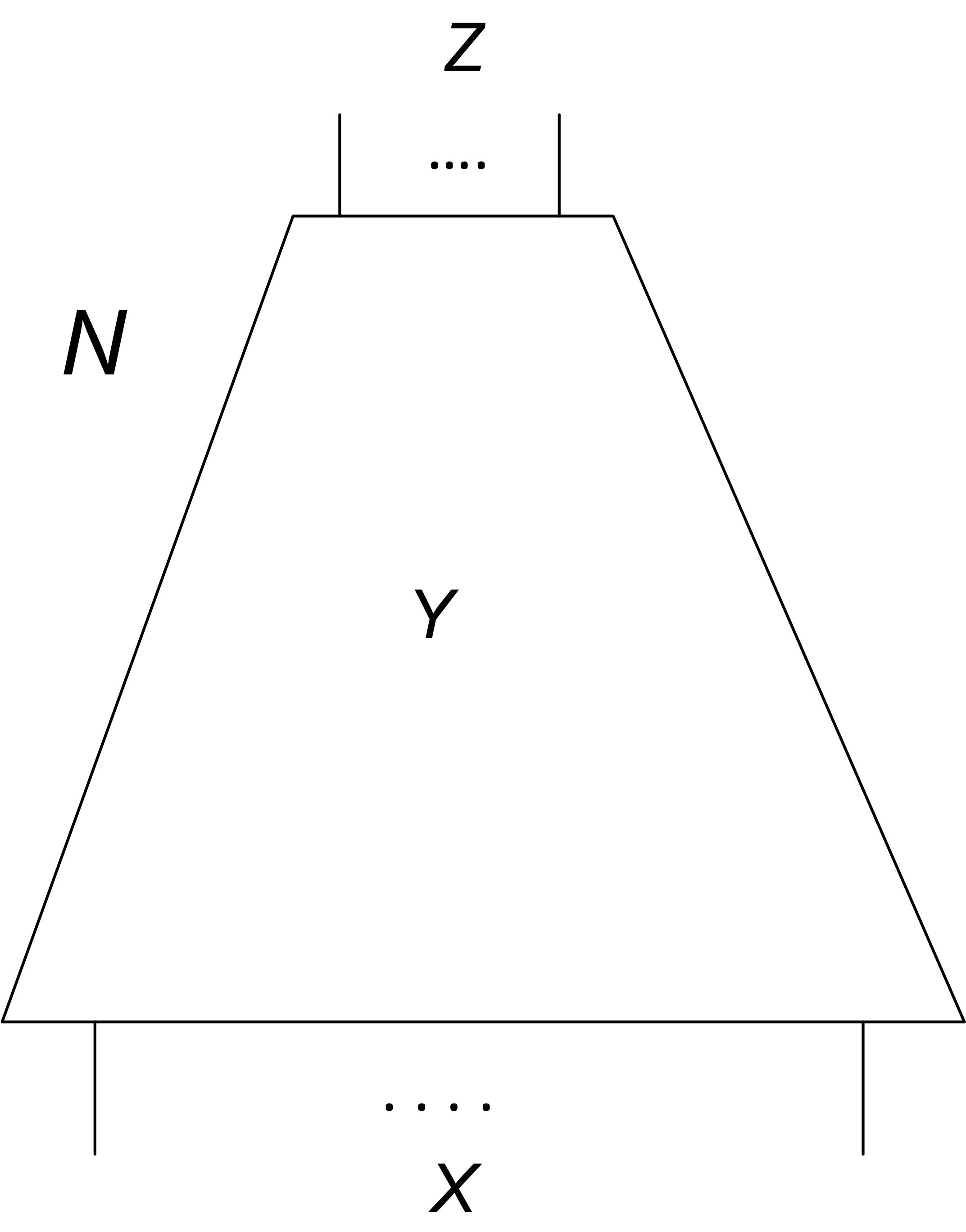
Let $N(X,Y,Z)$ be a combinational circuit where $X,Y,Z$ are the sets of input, intermediate and output variables of $N$ respectively (see Figure 1). We will refer to the set of all outputs produced by $N$ as the range of $N$. By an “output” here we mean a complete assignment of values to the variables of $Z$. We will also use term “input” to denote a complete assignment to the variables of $X$.

Suppose that one excludes a set $K$ of complete assignments to $X$ from the set of available inputs to $N$. If an output $z$ is produced only by inputs that are in $K$, excluding the inputs of $K$ from consideration leads to disappearance of $z$ from the range of $N$. The CRR problem is to compute the outputs of $N$ that are excluded from the range of $N$ if the inputs of a set $K$ are excluded from consideration.

Equivalence Checking can be a hard problem even for combinational circuits. This is especially true when the circuits to be compared have few functionally equivalent internal points. Our motivation here is that, as we argue in Section IV, equivalence checking by CRR facilitates construction of “natural” proofs. Such proofs are generated by industrial equivalence checkers when the circuits to be compared have a lot of internal points that are functionally equivalent.

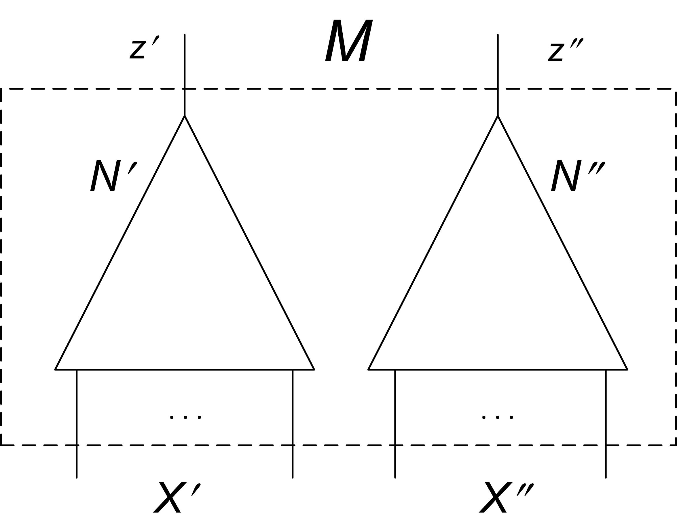
Application of CRR to equivalence checking is based on the following observation. Let $N^{\prime}$ and $N^{\prime\prime}$ be single-output combinational circuits to be checked for equivalence. (The expression “a single-output circuit” means that this circuit has only one output variable. Whether we use term “output” to refer to an “output variable” or “output assignment” should be clear from the context.) Let $M$ be a two-output circuit composed of $N^{\prime}$ and $N^{\prime\prime}$ as shown in Figure 2. Note that the sets $X^{\prime}$ and $X^{\prime\prime}$ of input variables of $N^{\prime}$ and $N^{\prime\prime}$ are independent of each other. Then, if $N^{\prime}$ and $N^{\prime\prime}$ are not constants, the range of circuit $M$ consists of all four assignments to the output variables $z^{\prime}$,$z^{\prime\prime}$ of $N^{\prime}$ and $N^{\prime\prime}$.

Let ($x^{\prime}$,$x^{\prime\prime}$) denote an assignment to variables $X^{\prime}\cup X^{\prime\prime}$. Suppose that one excludes from consideration all assignments ($x^{\prime}$,$x^{\prime\prime}$) where ${\mbox{\boldmath$x^{\prime}$}}\neq{\mbox{\boldmath$x^{\prime\prime}$}}$. Then if $N^{\prime}$ and $N^{\prime\prime}$ are functionally equivalent, such constraint on inputs of $M$ should lead to disappearing assignments $(z^{\prime}=0,z^{\prime\prime}=1)$ and $(z^{\prime}=1,z^{\prime\prime}=0)$ from the range of $M$. If this is not the case, then there is an input ($x^{\prime}$,$x^{\prime\prime}$) of $M$ where $x^{\prime}$=$x^{\prime\prime}$ for which $N^{\prime}$ and $N^{\prime\prime}$ evaluate to different values i.e. $N^{\prime}$ and $N^{\prime\prime}$ are inequivalent.

Functional verification of a combinational circuit $N$ comes down to checking if the range of $N$ contains an erroneous output. The straightforward approach of computing the range of $N$ is extremely inefficient. Simulation can be viewed as a way to simplify the range computation problem by reducing the set of inputs of $N$ to only one (regular simulation) or to a subset of inputs (symbolic simulation [2]). In this paper, we consider a different way to cope with complexity of range computation called simulation-by-exclusion. It is based on the idea of computing the reduction of range of $N$ caused by excluding some inputs from consideration rather than the entire range of $N$.

Suppose that one needs to check if an erroneous output $z$ is produced by $N$. Assume that a set of inputs $K$ is excluded from consideration. Let $Q$ be the set of outputs that disappear from the range of $N$ due to exclusion of inputs from $K$. One can have only the following two cases. The first case is ${\mbox{\boldmath$z$}}\not\in Q$. This means that either $z$ is not in the range of $N$ i.e. $N$ is correct or $N$ is buggy but there is an input ${\mbox{\boldmath$x$}}\not\in K$ producing $z$. So exclusion of the inputs of $K$ does not make $z$ disappear from the range of $N$. Then one can safely remove the inputs of $K$ from further consideration because if $N$ is buggy, the set of available inputs still contains a counterexample. The second case is ${\mbox{\boldmath$z$}}\in Q$. Then $N$ is buggy because $z$ is in its range.

In this paper, we describe the basic algorithm of simulation-by-exclusion and a few of its modifications.

In [5], we showed that the CRR problem comes down to Partial Quantifier Elimination (PQE). The difference between partial and complete elimination is that, in PQE, only a part of the formula is taken out of the scope of quantifiers. Let us explain the relation between CRR and PQE in the context of equivalence checking. Let $\mathit{EQ}(X^{\prime},X^{\prime\prime})$ denote a propositional formula such that $\mathit{EQ}({\mbox{\boldmath$x^{\prime}$}},{\mbox{\boldmath$x^{\prime\prime}$}})=1$ iff $x^{\prime}$ = $x^{\prime\prime}$. Equivalence checking by CRR comes down to taking $\mathit{EQ}$ out of the scope of quantifiers in formula $\exists{W}[\mathit{EQ}\wedge F^{\prime}\wedge F^{\prime\prime}]$. Here formulas $F^{\prime}$ and $F^{\prime\prime}$ specify circuits $N^{\prime}$ and $N^{\prime\prime}$ of Figure 2 and $W=X^{\prime}\cup X^{\prime\prime}\cup Y^{\prime}\cup Y^{\prime\prime}$.

Taking $\mathit{EQ}$ out of the scope of quantifiers means finding a quantifier-free formula $H(z^{\prime},z^{\prime\prime})$ such that $\mbox{$\exists{W}[\mathit{EQ}\wedge F^{\prime}\wedge F^{\prime\prime}]$}\equiv H\wedge\mbox{$\exists{W}[F^{\prime}\wedge F^{\prime\prime}]$}$. If an output of circuit $M$ of Figure 2 disappears from its range after excluding inputs falsifying $\mathit{EQ}$, this output falsifies $H$. So if $H(0,1)=H(1,0)=0$, circuits $N^{\prime}$ and $N^{\prime\prime}$ are equivalent.

Let us explain the benefits of solving PQE. We assume here and henceforth that all formulas are represented in the Conjunctive Normal Form (CNF). The appeal of PQE is that it allows one to focus on deriving implications that matter. Namely, formula $H$ can be built solely from clauses that are implied by formula $\mathit{EQ}\wedge F^{\prime}\wedge F^{\prime\prime}$ and are not implied by formula $F^{\prime}\wedge F^{\prime\prime}$. This means that a PQE solver can ignore the resolvents obtained only from clauses of $F^{\prime}\wedge F^{\prime\prime}$ focusing on resolvents that are descendants of clauses of $\mathit{EQ}$. Such zooming in on the “right” resolvents can make building formula $H$ much more efficient.

Our methods of using CRR for equivalence checking and simulation are different in one important aspect. In equivalence checking, one builds a circuit $M$ of Figure 2 and eliminates the spurious behaviors where ${\mbox{\boldmath$x^{\prime}$}}\neq{\mbox{\boldmath$x^{\prime\prime}$}}$. The presence of a bug corresponds to the situation when an erroneous output is not excluded from the range of $M$ under the input constraints. Conversely, simulation-by-exclusion is based on elimination of valid inputs. Then, the presence of a bug corresponds to the situation where an erroneous output is excluded from the range of the circuit under test.

The difference above is important for the following reason. When describing application of CRR to equivalence checking and simulation in Subsections  I-B and I-C we assumed that range reduction is computed precisely. However, a PQE solver computes a superset of the set of excluded outputs  [5] that may include outputs that are not in the range (see Subsection III-D.) We will refer to such outputs as noise. Adding noise to the set of excluded outputs in equivalence checking by CRR cannot trigger false alarms. (As we mentioned above the situation of concern here is when a bad output of $M$ is not excluded under input constraints. ) Conversely, in simulation-by-exclusion, adding noise can set off a false alarm. This happens when a bad output $z$ is in the set of excluded outputs computed by a PQE solver but, in reality, $z$ is not in the range of the circuit.

This paper is structured as follows. Section II formally defines the CRR problem. Solving this problem by PQE is discussed in Section III. In Section IV, we introduce a method of equivalence checking by CRR. Simulation-by-exclusion is discussed in Sections V and  VI. Some background and conclusions are given in Section VII and Section VIII respectively.

Given a quantified CNF formula $\exists{W}[F(V,W)]$, the problem of Quantifier Elimination (QE) is to find a quantifier-free formula $H(V)$ such that $H\equiv\mbox{$\exists{W}[F]$}$.

Given a quantified CNF formula $\exists{W}[G(V,W)\wedge F(V,W)]$, the problem of Partial Quantifier Elimination (PQE) is to find a quantifier-free CNF formula $G^{*}(V)$ such that $G^{*}\wedge\mbox{$\exists{W}[F]$}\equiv\mbox{$\exists{W}[G\wedge F]$}$. We will say that formula $G^{*}$ is obtained by taking $G$ out of the scope of quantifiers in $\exists{W}[G\wedge F]$. The term “partial” emphasizes the fact that, in contrast to QE, only a part of the quantified formula is taken out of the scope of quantifiers.

In this paper, we do not discuss algorithms for solving the PQE problem. In Subsection IV-B, we only explain how a PQE algorithm implements a cut advancement strategy. More information can be found in  [6].

Let $F(X,Y,Z)$ be a CNF formula specifying circuit $N(X,Y,Z)$. That is every consistent assignment of Boolean values to variables of $N$ is a satisfying assignment for $F$ and vice versa. Let $H(Z)$ be a CNF formula such that $H\equiv\mbox{$\exists{X}\exists{Y}[F]$}$. Then the outputs of $N$ satisfying $H$ specify the range of $N$. So computing the range of $N$ comes down to solving the QE problem. Assume that only inputs satisfying formula $G(X)$ are considered. Then a CNF formula $H(Z)$ equivalent to $\exists{X}\exists{Y}[G\wedge F]$ specifies the range of $N$ under inputs satisfying $G$.

Suppose that we are interested only in finding how the range of $N$ reduces if the inputs falsifying $G$ are excluded i.e. only inputs satisfying $G$ are considered. As we showed in  [5], this problem comes down to finding CNF formula $G^{*}(Z)$ such that $G^{*}\wedge\mbox{$\exists{W}[F]$}\equiv\mbox{$\exists{W}[G\wedge F]$}$ where $W=X\cup Y$. Here $G^{*}$ specifies an approximate solution to the CRR problem (see Definition 2) i.e.

• •

  the outputs falsifying $G^{*}$ specify a superset of the set of outputs disappearing from the range of $N$ due to excluding inputs falsifying $G$

• •

  every output $z$ falsifying $G^{*}$ either disappeared from the range of $N$ due to excluding inputs falsifying $G$ or is not in the range of $N$

As we mentioned above, computing the range of $N$ reduces to QE whereas finding range reduction comes down to PQE. So the complexity of computing range and range reduction is directly related to that of QE and PQE.

The difference between QE and PQE can be expressed in terms of computing clause redundancy [4, 6]. For the sake of simplicity, in descriptions of algorithms of  [4] and  [6] given below we omitted the fact that they use branching. (First the problem is solved in subspaces. Then the results of branches are merged to produce a solution that holds for the entire search space.)

As we showed in [3, 4], to eliminate quantifiers from $\exists{W}[F(X,Y,Z)]$ where $W=X\cup Y$ one needs to find a CNF formula $H(Z)$ implied by $F$ that makes all the clauses of $F$ with quantified variables redundant in $\exists{W}[F\wedge H]$. Then formula $H$ is logically equivalent to $\exists{W}[F]$. We will refer to clauses containing variables of $W$ (i.e. quantified variables) as $W$-clauses.

Clauses of $H$ are built from $F$ by adding resolvent clauses. If a resolvent is a $W$-clause, its redundancy has to be proved along with the original $W$-clauses of $F$. Eventually, a sufficient number of clauses depending only on free variables (i.e. those of $Z$) is added to make the new and old $W$-clauses of $F$ redundant.

Now, let us consider the PQE problem of taking formula $G(X)$ out of the scope of quantifiers in $\exists{W}[G\wedge F]$. As we showed in [6], this problem comes down to finding formula $G^{*}(Z)$ implied by $G\wedge F$ that makes redundant the clauses of $G$ in $\exists{W}[G^{*}\wedge G\wedge F]$. The clauses of $G^{*}$ are built by resolving clauses of $G\wedge F$. If a resolvent is a $W$-clause and is a descendant of a clause of $G$, its redundancy needs to be proved as well. On the other hand, $W$-resolvents produced solely from clauses of $F$ do not need to be proved redundant. This can make PQE drastically simpler than QE if $G$ is much smaller than $F$.

In this subsection, we clarify the relation between the quality of a PQE-algorithm and that of an approximate solution to the CRR problem. As in the previous subsection, we assume that formula $G^{*}(Z)$ is obtained by taking formula $G(X)$ out of the scope of quantifiers in $\exists{W}[G\wedge F]$. Here $W=X\cup Y$ and $F$ specifies circuit $N(X,Y,Z)$.

The definitions below are based on the following observation. If $G^{*}$ is a solution to the PQE problem above, a formula obtained by adding to $G^{*}$ a clause $C(Z)$ implied by $F$ is also a solution to the PQE problem. One can view $C$ as “noise”. Such a clause is falsified only by outputs that are not in the range of $N$. In general, the set of outputs falsifying a clause of $G^{*}$ can contain outputs that are in the range of $N$ and those that are not.

The intuition behind applying CRR to equivalence checking was described in the introduction. In this subsection, we substantiate this intuition in a formal proposition.

Let $N^{\prime}(X^{\prime},Y^{\prime},z^{\prime})$ and $N^{\prime\prime}(X^{\prime\prime},Y^{\prime\prime},z^{\prime\prime})$ be single-output combinational circuits to be checked for equivalence. Let $M(X^{\prime},X^{\prime\prime},Y^{\prime},Y^{\prime\prime},z^{\prime},z^{\prime\prime})$ be the circuit composed of $N^{\prime}$ and $N^{\prime\prime}$ as shown in Figure 2. Let $F^{\prime}(X^{\prime},Y^{\prime},z^{\prime})$ and $F^{\prime\prime}(X^{\prime\prime},Y^{\prime\prime},z^{\prime\prime})$ be CNF formulas specifying $N^{\prime}$ and $N^{\prime\prime}$ respectively. Assume that $X^{\prime}=\mbox{$\{x^{\prime}_{1},\dots,x^{\prime}_{k}\}$}$ and $X^{\prime\prime}=\mbox{$\{x^{\prime\prime}_{1},\dots,x^{\prime\prime}_{k}\}$}$. Denote by $\mathit{EQ}(X^{\prime},X^{\prime\prime})$ formula $(x^{\prime}_{1}\equiv x^{\prime\prime}_{1})\wedge\dots\wedge(x^{\prime}_{k}\equiv x^{\prime\prime}_{k})$ that is satisfied by inputs $x^{\prime}$ and $x^{\prime\prime}$ to $N^{\prime}$ and $N^{\prime\prime}$ iff $x^{\prime}$ = $x^{\prime\prime}$.

In this subsection, we compare equivalence checking by a SAT-solver with Conflict Driven Clause Learning (CDCL) and by CRR.

The equivalence checking of circuits $N^{\prime}(X^{\prime},Y^{\prime},z^{\prime})$ and $N^{\prime\prime}(X^{\prime\prime},Y^{\prime\prime},z^{\prime\prime})$ can be performed by checking the satisfiability of formula $F$ equal to $F^{\prime}(X,Y^{\prime},z^{\prime})\wedge F^{\prime\prime}(X,Y^{\prime\prime},z^{\prime\prime})\wedge(z^{\prime}\neq z^{\prime\prime})$. Indeed, the existence of an assignment ${\mbox{\boldmath$x$}},{\mbox{\boldmath$y^{\prime}$}},{\mbox{\boldmath$y^{\prime\prime}$}},z^{\prime},z^{\prime\prime}$ satisfying $F$ means that $N^{\prime}$ and $N^{\prime\prime}$ produce different output values for the same input $x$. We will refer to the method of equivalence checking by a SAT solver based on CDCL solver as EC_CDCL. Here EC stands for Equivalence Checking.

Proposition 1 justifies the following method of equivalence checking by CRR. We will refer to this method as EC_CRR. This method solves the PQE problem specified by formula $F$ equal to $\exists{W}[\mbox{$\mathit{EQ}(X^{\prime},X^{\prime\prime})$}\wedge F^{\prime}(X^{\prime},Y^{\prime},z^{\prime})\wedge F^{\prime\prime}(X^{\prime\prime},Y^{\prime\prime},z^{\prime\prime})]$ where $W=X^{\prime}\cup X^{\prime\prime}\cup Y^{\prime}\cup Y^{\prime\prime}$. Namely, EC_CRR computes formula $H(z^{\prime},z^{\prime\prime})$ obtained by taking $\mathit{EQ}$ out of the scope of quantifiers in $\exists{W}[EQ\wedge F^{\prime}\wedge F^{\prime\prime}]$. If $H(0,1)=H(1,0)=0$, then $N^{\prime}$ and $N^{\prime\prime}$ are equivalent. Otherwise, one needs to check if $N^{\prime}$ and $N^{\prime\prime}$ are identical constants. If so, then $N^{\prime}$ and $N^{\prime\prime}$ are equivalent, otherwise they are not. Theoretically, proving $N^{\prime}$ and $N^{\prime\prime}$ inequivalent does not require generation of a counterexample. The very fact that $H(0,1)=1$ or $H(1,0)=1$ and $N^{\prime},N^{\prime\prime}$ are not constants guarantees that $N^{\prime}$ and $N^{\prime\prime}$ are not equivalent. However, in a practical implementation of EC_CRR, a counterexample may be generated before computation of formula $H$ is completed.

To distinguish the formulas $F$ solved by EC_CDCL and EC_CRR, we will refer to them as $F^{\mathit{cdcl}}$ and $F^{\mathit{crr}}$ respectively. The SAT problem can be viewed as a special case of QE where all variables of the formula are existentially quantified. Since EC_CRR  is actually a PQE algorithm, one can compare EC_CRR  and EC_CDCL  in terms of computing clause redundancy as we did Subsection III-C. In those terms, the objective of deriving an empty clause by a SAT-solver is to make redundant all clauses with quantified variables (i.e. all clauses containing literals). So the difference between EC_CDCL  and EC_CRR  is that the former is aimed at making redundant all clauses of $F^{\mathit{cdcl}}$ while the goal of the latter is to make redundant only a small subset of clauses of $F^{\mathit{crr}}$ (namely those of $\mathit{EQ}$).

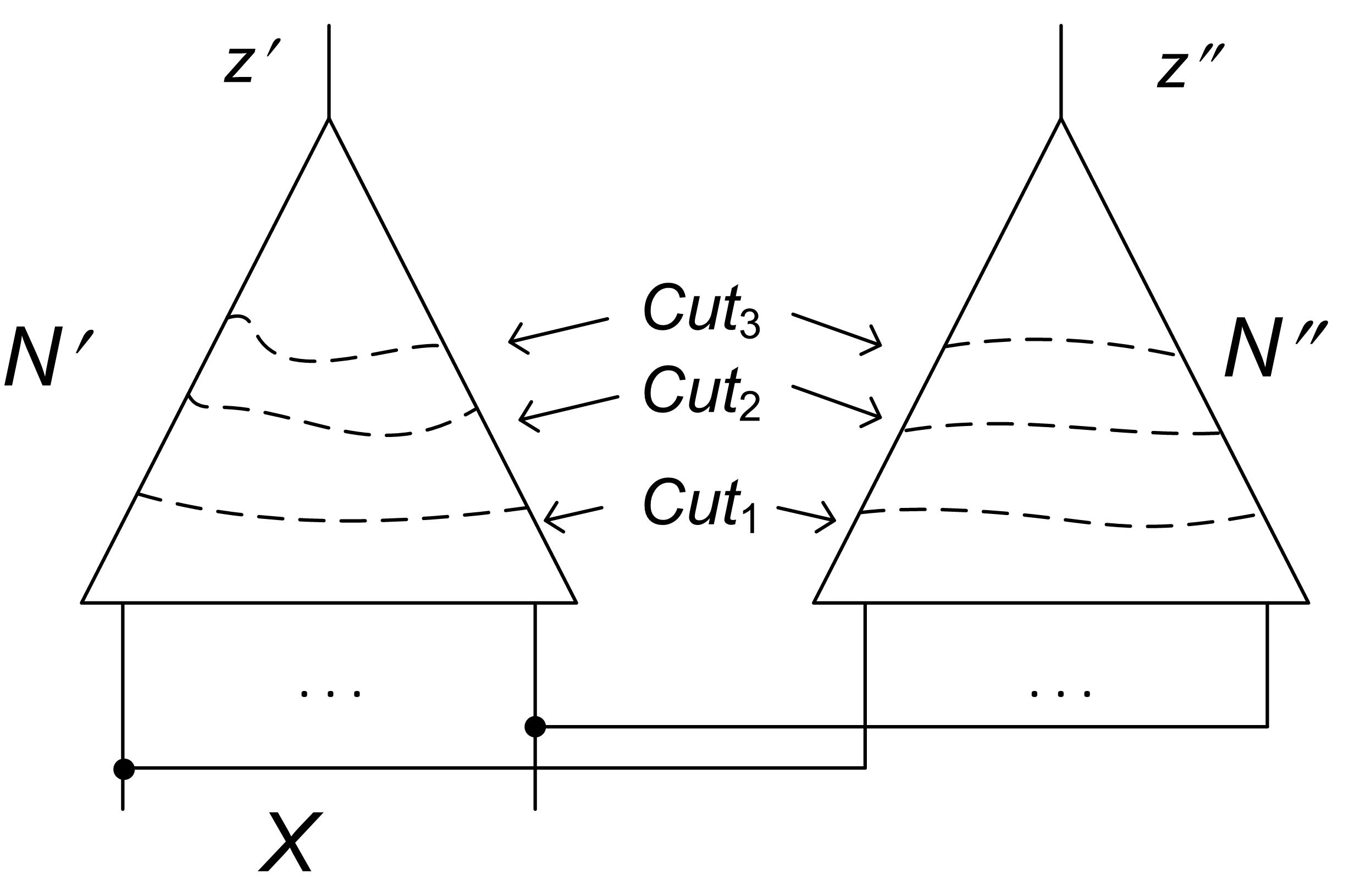
The fact that EC_CRR  needs to prove redundancy of a smaller set of clauses than EC_CDCL  does not necessarily imply greater efficiency of EC_CRR. What matters, though, is that solving the PQE problem specified by $F^{\mathit{crr}}$ facilitates generation of proofs based on the cut advancement strategy shown in Figure 3. Such proofs are natural for structurally similar circuits. Here is a naive version of how this works. To make clauses of $\mathit{EQ}$ redundant one just needs to produce new clauses obtained by resolving $\mathit{EQ}$ with those of $F^{\prime}\wedge F^{\prime\prime}$. Note that a PQE solver has to make redundant a new resolvent (depending on a quantified variable) only if it is a descendant of a clause from $\mathit{EQ}$. In general, such a clause will contain variables of both $F^{\prime}$ and $F^{\prime\prime}$ relating variables of $N^{\prime}$ and $N^{\prime\prime}$. The set $G_{1}$ of new resolvents that made the clauses of $\mathit{QE}$ redundant specify a new “cut” that consists of the variables present in $G_{1}$. After that a set $G_{2}$ of descendants of $G_{1}$ that make the clauses of $G_{1}$ redundant is built. This goes on until the cut consisting of variables $z^{\prime}$ and $z^{\prime\prime}$ is reached.

A cut advancement strategy has been successfully used by industrial equivalence checkers. However, it is applied only when $N^{\prime}$ and $N^{\prime\prime}$ are so structurally similar that one can build a cut consisting of internal points of $N^{\prime}$ and $N^{\prime\prime}$ that are functionally equivalent. So this version of cut advancement is very limited. On the other hand, EC_CRR can arguably extend the cut advancement strategy to a much more general class of equivalence checking problems.

Let $F(X,Y,Z)$ be a CNF formula specifying circuit $N$. Computing the range of $N$ comes down to finding formula $H(Z)$ logically equivalent to $\exists{W}[F]$ where $W=X\cup Y$. Simulation can be viewed as a way to decrease the complexity of finding $H(Z)$ by shrinking the set of allowed inputs to only one. Let $S(X)$ be a CNF formula satisfied by only one input $x$. Then computing the output produced by $N$ comes down to solving the QE problem $\exists{W}[S\wedge F]$. Formula $S$ can be represented as a set of $|X|$ unit clauses satisfied only by $x$. (A clause is called unit if it contains exactly one literal.) A solution $H(Z)$ for this QE problem can be represented as a set of $|Z|$ unit clauses satisfied only by the output of $N$ for input $x$.

An obvious flaw of traditional simulation is that it provides information about the value of $N$ only for one input out of $2^{|X|}$. One can address this issue by using formulas $S$ with many satisfying assignments, Then solving the QE problem specified by $\exists{W}[S\wedge F]$ finds the range of $N$ where all inputs satisfying $S$ are processed together. Unfortunately, the complexity of QE grows very fast as the number of inputs satisfying $S$ increases. One way to reduce the complexity of QE when $S$ allows many inputs is employed in symbolic simulation [2]. The idea is to pick formulas $S$ for which all inputs satisfying $S$ have the same execution trace.

We described the main idea of simulation-by-exclusion in Subsection I-C. Given constraints excluding some inputs, compute only reduction of range of $N$ caused by this exclusion rather than the entire range of $N$ under allowed inputs. Here we continue explanation describing how simulation-by-exclusion is implemented by PQE. Let the complete assignments to $X$ falsifying CNF formula $Q(X)$ specify the inputs excluded from consideration. Let CNF formula $Q^{*}(Z)$ be obtained by taking $Q(X)$ out of the scope of quantifiers in $\exists{W}[Q\wedge F]$ where $W=X\cup Y$. Then the outputs falsifying $Q^{*}$ specify the range reduction of $N$ due to exclusion of inputs falsifying $Q$.

Suppose that no output falsifying $Q^{*}$ is in the set $E$ of erroneous outputs of $N$. This implies that either $N$ is correct or there is an input $x$ producing an output from $E$ (a counterexample) that is not excluded i.e. $x$ satisfies $Q$. This means that removing all inputs falsifying $Q$ from consideration is safe because it cannot remove all counterexamples (if any).

As we mentioned earlier, a PQE solver provides only an approximate solution to the CRR problem. This means that even if an output $z$ falsifying $Q^{*}$ is in $E$, one still needs to check if $z$ is in the range of $N$. A trivial way to do it is to check if formula $\overline{\mbox{$C_{\boldsymbol{z}}$}}\wedge F$ is satisfiable where $C_{\boldsymbol{z}}$ is the longest clause falsified by $z$. If so, clause $C_{\boldsymbol{z}}$ is not implied by $F$ and $z$ is in the range of $N$.

Checking the satisfiability of $\overline{\mbox{$C_{\boldsymbol{z}}$}}\wedge F$ may be expensive. However, in the algorithm of simulation-by-exclusion we introduce in Section VI, formula $F$ is constantly updated by adding clauses excluding inputs of $N$. This may drastically simplify the SAT-check above. Besides, there are at least two techniques to make this SAT-check even simpler. The first technique is based on the fact that all inputs producing $z$ (if any) falsify $Q$. So checking if $z$ is in the range of $N$ reduces to testing the satisfiability $\overline{Q}\wedge\overline{\mbox{$C_{\boldsymbol{z}}$}}\wedge F$.

The second technique is based on the following observation. Let $R$ be a resolution derivation of a clause $C$ of $Q^{*}$ falsified by $z$. Then if $z$ is in the range of $N$, every cut $\mathit{Cut}(R)$ of proof $R$ has to include at least one clause $A$ that is implied by $Q\wedge F$ but not $F$. (We assume here that $R$ is a directed graph nodes of which correspond to original clauses of $Q\wedge F$ or resolvents.) If every clause of $\mathit{Cut}(R)$ is implied by $F$ then the clause $C$ derived by $R$ is implied by $F$ too and so $z$ is not in the range of $N$. So to find out if $z$ is in the range of $N$ it is sufficient to check if formula $\overline{A}\wedge\overline{Q}\wedge\overline{\mbox{$C_{\boldsymbol{z}}$}}\wedge F$ is satisfiable for every clause $A$ of $\mathit{Cut}(R)$. The longer clause $A$ is the simpler this SAT-check. If all such formulas are unsatisfiable for $\mathit{Cut}(R)$ then $z$ is not in the range of $N$. Otherwise, an input of $N$ producing $z$ can be extracted from an assignment satisfying formula $\overline{A}\wedge\overline{Q}\wedge\overline{\mbox{$C_{\boldsymbol{z}}$}}\wedge F$.

In this subsection, term “regular simulation” refers to finding a solution $H(Z)$ to the QE problem specified by $\exists{W}[Q\wedge F]$ that we introduced in Subsection V-A (see also Footnote 1).

The main difference between regular simulation and simulation-by-exclusion is as follows. In regular simulation, to get a result one needs to perform a computation that goes all the way from inputs to outputs. If only one input $x$ is allowed by $Q$, this computation produces an execution trace consisting of values assigned to variables of $N$ when applying input $x$. On the other hand, simulation-by-exclusion can get a valuable result even by a local computation that does not reach the outputs of $N$.

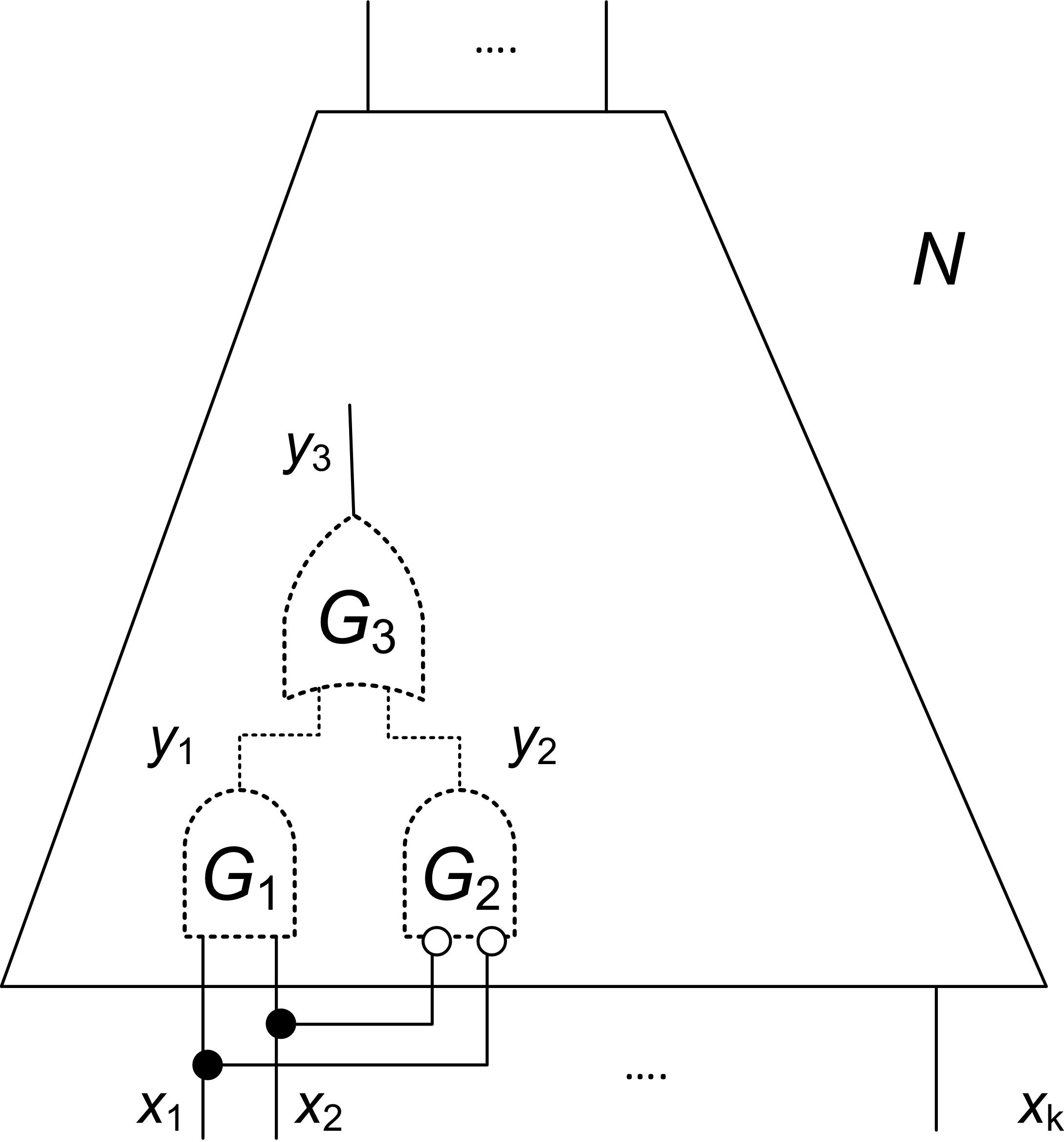
Let us consider the example of Figure 4 showing a circuit $N$. Suppose that lines $x_{1},x_{2}$ feed only gates $G_{1}$ and $G_{2}$ and lines $y_{1},y_{2}$ feed only gate $G_{3}$. Note that the output of $G_{3}$ specified by $y_{3}$ implements function $x_{1}\equiv x_{2}$ i.e. $y_{3}=1$ iff values of $x_{1}$ and $x_{2}$ are equal. Let $C$ denote clause $x_{1}\vee x_{2}$. It is not hard to show that $C$ is redundant in formula $\exists{W}[C\wedge F]$ i.e. $\mbox{$\exists{W}[C\wedge F]$}\equiv\mbox{$\exists{W}[F]$}$. The redundancy of $C$ means that one can exclude the inputs falsifying $C$ (i.e. all the inputs for which $x_{1}=0,x_{2}=0$) from consideration because such exclusion does not change the range of $N$. Indeed, since $x_{1},x_{2},y_{1},y_{2}$ feed only gates $G_{1},G_{2},G_{3}$, circuit $N$ produces the same output for two inputs that are different only in the values of $x_{1}$ and/or $x_{2}$ if these inputs produce the same assignment to $y_{3}$. Since, even after excluding assignment $x_{1}=0,x_{2}=0$, both values of $y_{3}$ can still be produced, the set of outputs circuit $N$ can generate remains intact.

Importantly, the fact that clause $C$ can be safely used to exclude inputs of $N$ is derived locally without any knowledge of the rest of the circuit $N$. Such a result cannot be reproduced efficiently by regular simulation. To exclude the inputs falsified by $C$ from consideration one would need to solve the QE problem specified by $\exists{W}[\overline{C}\wedge F]$. The complexity of such QE can be very high if the size of circuit $N$ is large. Of course, if regular simulation succeeds in performing QE, it might find a bug. However, if no bug is found, the result is the same as for simulation-by-exclusion: the inputs falsifying $C$ can be excluded. However the price of this result in regular simulation can be dramatically higher than in simulation-by-exclusion.

The algorithm of simulation-by-exclusion called SimByExl consists of three parts separated in Figure 5 by the dotted lines. In the first part (lines 1-6), an input $\hat{x}$ is generated for which $N$ evaluates to 0 (lines 2-4). This input is never excluded and serves two purposes. First, it guarantees that $N$ is not a constant 1. Second, keeping $\hat{x}$ allowed prevents SimByExcl  from excluding all inputs for which $N$ evaluates to 0. SimByExcl also builds formula $F$ specifying $N$ (line 1) and generates $C_{\boldsymbol{\hat{x}}}$, the longest clause falsified by $\hat{x}$ (line 5). Finally, SimByExcl initializes formula $G$ that accumulates the clauses excluding inputs of $N$ (line 6).

The second part of SimByExcl  (lines 7-14) consists of a while loop. In every iteration of this loop, a new clause $C(X)$ is generated (line 10). Clause $C$ excludes at least one new input $x$ of $N$ constructed as an assignment satisfying formula $G\wedge\mbox{$C_{\boldsymbol{\hat{x}}}$}$ (line 8). If SimByExcl fails to find such $x$, all inputs of $N$ but $\hat{x}$ have been excluded. Then $N$ is correct since, for the excluded inputs, it takes the same value as for $\hat{x}$ i.e. 0.

After generating clause $C$, SimByExcl computes CNF formula $C^{*}(z)$ (line 11). It is obtained by taking $C$ out of the scope of quantifiers in $\exists{W}[C\wedge F]$ where $W=X\cup Y$. Formula $C^{*}$ can only consist of clause $\overline{z}$ or be empty (no clauses) in which case $C^{*}$ is always true. Note that formula $C^{*}$ cannot consist of unit clause $z$ because SimByExcl never excludes all inputs for which $N$ evaluates to 0. Hence clause $z$ is not implied by $C\wedge F$. If $C^{*}$ is empty, then the inputs falsifying $C$ can be safely excluded from consideration. So clause $C$ is added to $F$ (line 13) and to $G$ (line 14).

If $C^{*}$ is not empty and hence equal to $\overline{z}$, SimByExcl breaks the loop (line 12) and executes the third part of the algorithm (lines 15-17). In this part, SimByExcl checks whether the derived clause $\overline{z}$ is pure noise or $C$ excludes a counterexample. If no counterexample is excluded by $C$, then clause $\overline{z}$ is just noise, i.e. $F\rightarrow\overline{z}$ and so $N$ is correct. Otherwise, SimByExcl extracts a counterexample from an assignment satisfying $\overline{C}\wedge F\wedge z$.

Note that one can just check whether $N$ is constant 0 by running the SAT-check on $F\wedge z$ where $F$ is the original formula specifying $N$. SAT-checking of $F\wedge z\wedge\overline{C}$ can be much simpler for the following two reasons. First, $F$ is constantly updated by SimByExcl  by adding clauses excluding inputs. As we explain in Subsection VI-C such clauses are obtained by non-resolution derivation and so are very valuable for a resolution-based SAT-solver. Second, the negation of clause $C$ consists of unit clauses that can additionally simplify the SAT-check. One more way to simplify this SAT-check that we described in Subsection V-B is to exploit the resolution derivation of clause $\overline{z}$. For the sake of simplicity this possibility is not mentioned in Figure 5.

SimByExcl produces an answer for every circuit $N$ and so it is complete. Indeed, in every iteration of the while loop, SimByExcl excludes at least one new input of $N$ that has not been excluded so far. So the set of allowed inputs monotonically decreases. Eventually, SimByExcl either excludes all inputs but $\hat{x}$ or derives a clause $\overline{z}$. In either case, SimByExcl terminates returning a result.

SimByExcl is sound. It reports that $N$ is correct in two cases. First, when a clause $\overline{z}$ is generated and SimByExcl proves that $F\rightarrow\overline{z}$. Then $F\wedge z$ is unsatisfiable and hence no counterexample exists. Second, SimByExcl reports that $N$ is correct when all inputs of $N$ but $\hat{x}$ are excluded by added clauses. Since SimByExcl  guarantees that a new clause cannot remove all counterexamples and $N$ evaluates to 0 at $\hat{x}$, this means that $N$ evaluates to 0 for all inputs. SimByExcl reports that $N$ is buggy when an assignment satisfying $F\wedge z$ is found. This assignment specifies an input for which $N$ evaluates to 1.

In this subsection, we consider two modifications of SimByExcl  that can be used to improve its efficiency. The first modification is given in Figure 6. The high-lighted part shows the lines added to the code of SimByExcl of Figure 5.

The main idea here is to occasionally run a light SAT-check on formula $F\wedge z$. We assume that the effort of the SAT-solver is limited by some parameter specifying e.g. the maximum number of backtracks. Such a SAT-check is invoked when the number of new clauses added to $F$ exceeds a threshold. Such a strategy makes sense because clauses added to $F$ by SimByExcl are not derived by resolution. Deriving such clauses by resolution may be dramatically more complex, which makes them quite valuable for a resolution based SAT-solver.

Consider for instance, derivation of clause $C=x_{1}\vee x_{2}$ for circuit $N$ shown in Figure 4 (see discussion of Subsection V-C). Assume that circuit $N$ has only one output specified by variable $z$. Suppose that formula $F\wedge z$ is satisfiable (i.e. $N$ is buggy) and $C$ excludes at least one counterexample. Then $C$ is not even implied by $F\wedge z$ and thus cannot be derived by resolution. However, even if $C$ is implied by $F\wedge z$, its resolution derivation may be very hard and involve many clauses of $F$. On the other hand, a PQE-solver is capable of concluding that $C$ can be safely added to $F$ just by examining the clauses specifying gates $G_{1}$,$G_{2}$,$G_{3}$ and using the fact that variables $x_{1},x_{2},y_{1},y_{2}$ do not feed any other gates.

The second modification is shown in Figure 7. In this modification one occasionally runs regular simulation. We assume that only tests that have not been excluded yet are generated. These are the tests satisfying formula $G$. A simulation run is performed when the number of new clauses added to $G$ exceeds a threshold. We assume that the number of tests generated in a simulation run is limited by parameter #tries. Performing occasional simulation runs makes sense because adding new clauses reduces the search space and hence increases the probability of generating a counterexample.

References

- [1] R. Bryant. Graph-based algorithms for Boolean function manipulation. IEEE Transactions on Computers, C-35(8):677–691, August 1986.
- [2] R. Bryant. Symbolic simulation—techniques and applications. In DAC-90, pages 517–521, 1990.
- [3] E.Goldberg and P.Manolios. Quantifier elimination by dependency sequents. In FMCAD-12, pages 34–44, 2012.
- [4] E.Goldberg and P.Manolios. Quantifier elimination via clause redundancy. In FMCAD-13, pages 85–92, 2013.
- [5] E.Goldberg and P.Manolios. Bug hunting by computing range reduction. Technical Report arXiv:1408.7039 [cs.LO], 2014.
- [6] E. Goldberg and P. Manolios. Partial quantifier elimination. In Proc. of HVC-14, pages 148–164. Springer-Verlag, 2014.
- [7] E. Goldberg, M. Prasad, and R. Brayton. Using SAT for combinational equivalence checking. In DATE, pages 114–121, 2001.
- [8] O. Guzey and L.C. Wang. Coverage-directed test generation through automatic constraint extraction. In HLDVT.
- [9] A. Kuehlmann and F. Krohm. Equivalence Checking Using Cuts And Heaps. DAC, pages 263–268, 1997.
- [10] J. Marques-Silva and K. Sakallah. Grasp – a new search algorithm for satisfiability. In ICCAD-96, pages 220–227, 1996.
- [11] M. Moskewicz, C. Madigan, Y. Zhao, L. Zhang, and S. Malik. Chaff: engineering an efficient sat solver. In DAC-01, pages 530–535, New York, NY, USA, 2001.