ergodic and foliated kernel-differentiation method for linear responses of random systems
Abstract.
We extend the kernel-differentiation method (or likelihood-ratio method) for the linear response of random dynamical systems, after revisit its derivation in a microscopic view via transfer operators. First, for the linear response of physical measures, we extend the method to an ergodic version, which is sampled by one infinitely-long sample path; moreover, the magnitude of the integrand is bounded by a finite decorrelation step number. Second, when the noise and perturbation are along a given foliation, we show that the method is still valid for both finite and infinite time. We numerically demonstrate the ergodic version on a tent map, whose linear response of the physical measure does not exist; but we can add some noise and compute an approximate linear response. We also demonstrate on a chaotic neural network with 51 layers 9 neurons, whose perturbation is along a given foliation; we show that adding foliated noise incurs a smaller error than noise in all directions. We give a rough error analysis of the method and show that it can be expensive for small-noise. We propose a potential future program unifying the three popular linear response methods.
Keywords. likelihood ratio method, chaos, linear response, random dynamical systems.
AMS subject classification numbers. 37M25, 65D25, 65P99, 65C05, 62D05, 60G10.
1. Introduction
1.1. Literature review
The averaged statistic of a dynamical system is of central interest in applied sciences. The average can be taken in two ways. When the system is random, we can average with respect to the randomness. On the other hand, if the system runs for a long-time, we can average with respect to time. The long-time average can also be defined for deterministic systems, and the existence of the limit measure is called the physical measure or SRB measure [43, 38, 6]. If the system is both random and long time, the existence of the limit measure (which we shall also call the physical measure) is discussed in textbooks such as [11].
We are interested in the the linear response, which is the derivative of the averaged observable with respect to the parameters of the system. The linear response is a fundamental tool for many purposes. For example, in aerospace design, we want to know the how small changes in the geometry would affect the average lift of an aircraft, which was answered for non-chaotic fluids [23] but only partially answered for not-so-chaotic fluids [27]. In climate change, we want to ask what is the temperature change caused by a small change of level [16, 13]. In machine learning, we want to extend the conventional backpropagation method to cases with gradient explosion; current practices have to avoid gradient explosion but that is not always achievable [32, 22].
There are three basic methods for expressing and computing the linear response: the path perturbation method, the divergence method, and the kernel-differentiation method. The path perturbation method averages the path perturbation over a lot of orbits; this is also known as the ensemble method or stochastic gradient method (see for example [25, 12, 26]). However, when the system is chaotic, that is, when the pathwise perturbation grows exponentially fast with respect to time, the method becomes too expensive since it requires many samples to average a huge integrand. Proofs of such formula for the physical measure of hyperbolic systems were given in for example [39, 9, 24].
The divergence method is also known as the transfer operator method, since the perturbation of the measure transfer operator is some divergence. Traditionally, the divergence method is functional, and the formula is not pointwisely defined when the invariant measure is singular, which is common for systems with a contracting direction (see for example [19, 5]). This difficulty can not be circumvented by transformations such as Livisic theorem in [19]. Hence, the traditional divergence formulas can not be computed by a Monte-Carlo approach, so the computation is cursed by dimensionality (see for example [15, 42, 20, 2, 35]).
For chaotic deterministic systems, to have a formula without exponentially growing or distributive terms, we need to blend the two formulas, but the obstruction was that the split lacks smoothness. The ‘fast response’ linear response formulas solve this difficulty for deterministic hyperbolic systems. It is composed of two parts, the adjoint shadowing lemma [29] and the equivariant divergence formula [30]. The fast response formula is a pointwise defined function and has no exponentially growing terms. The continuous-time versions of fast response formulas can be found in [29, 31]. The fast response formula is the ergodic theorem for linear response: it computes -dimensional vectors on each point of an orbit, and then the average of some pointwise functions of these vectors. Here is the phase space dimension, and is the number of unstable directions.
The kernel-differentiation formula works only for random system. This method is more popularly known as the likelihood ratio method or the Monte-Carlo gradient method in probability context (see [37, 36, 17, 34]), the idea (dividing and multiplying the local density) is also used in Langevin sampling and diffusion models. However, such names are no longer distinguishing in the larger context: for example, the likelihood ratio idea is also useful in the divergence method. We apologize for the inconvenience in naming. Proofs of the kernel-differentiation method was given in [21, 3, 1]. This method is more powerful than the previous two for random dynamics, since annealed linear response can exist when quenched linear response does not [10]. However, as we shall see, inevitably, this method is expensive when the randomness is small, so it is hard to use this approach as a very good approximation to linear responses of deterministic systems.
In terms of numerics, the kernel-differentiation method naturally allows Monte-Carlo type sampling, so is efficient in high-dimensions. The formula does not involve Jacobian matrices hence does not incur propagations of vectors or covectors (parameter gradients), so it is not hindered by undesirable features of the Jacobian of the deterministic part, such as singularity or non-hyperbolicity. The work in [33] solves a Poisson equation for a term in the formula, which reduces the numerical error, but can be expensive for high-dimensions.
Another issue in previous likelihood ratio method is that the scale of the estimator is proportional to the orbit length. This leads to two undesirable consequences:
-
•
The requested number of sample orbits increases with orbit length.
-
•
We have to restart a new orbit very often. For each orbit, the observable function is only evaluated at the last step, while the earlier steps are somewhat wasted waiting for the orbits to land onto the physical measure.
This paper shows that, for physical measures, we can resolve these issues by invoking the decay of correlation and the ergodic theorem.
Moreover, sometimes we are interested in the case where some directions in the phase space have special importance, such as the level sets in Hamiltonian system. For these cases, the perturbation in the dynamics and the added noise are sometimes aligned to a subspace. This paper extends the kernel-differentiation method to foliated spaces.
Finally, for pedagogical purposes, it is beneficial to derive the kernel-differentiation method from a local or microscopic perspective. This will be somewhat more intuitive, and the above extensions will be more natural.
1.2. Main results
We consider the random dynamical system
Let and be the probability density for and . We need the expressions of ; but we do not need expressions of . We denote the density of the physical measure by , which is the limit measure under the dynamics. Here is the parameter controlling the dynamics and hence and ; by default . We denote the perturbation , and when is invertible, define
is a fixed observable function.
As a warm-up, through basic calculus, section 2.2 rederives the kernel-differentiation formula for , the linear response for 1-step. Section 2.3 gives a pictorial explanation for the main lemma. In this simplest setting, we can see more easily how the kernel-differentiation method relates to other methods, and why it can be generalized to foliated situations. Section 2.4 rederives the formula for finitely many steps, which was known as the likelihood ratio method and was given in [37, 36, 17]. Our derivation use the measure-transfer-operator point of view, which is more convenient for our extensions.
The first contribution of this paper, given in section 2.5, is the ergodic kernel-differentiation formula for physical measures. We invoke decay of correlations to constrain the scale of the estimator, and the ergodic theorem to reduce the required data to one long orbit. Hence, we only need to spend one spin-up time to land onto the physical measure, and then all data are fully utilized. This improves the efficiency of the algorithm. More specifically, we prove
[orbitwise kernel-differentiation formula for ] Under assumptions 1 and 2, we have
almost surely according to the measure obtained by starting the dynamic with . Here .
Here and are two separate and sequential limits, so we can typically pick . This makes the estimator smaller than previous likelihood ratio formulas, where . Our formula runs on only one orbit; hence, it is faster than previous likelihood ratio methods. Section 2.6 generalizes the result to cases where the randomness depends on locations and parameters.
The second contribution of this paper is that section 3 extends the kernel-differentiation method to the case where the phase space is partitioned by submanifolds, and the added noise and the perturbation are along the submanifolds (hence the noise is ‘singular’ with respect to the Lebesgue measure). More specifically, Let be a co-dimension foliation on , which is basically a collection of -dimensional submanifolds partitioning , and each submanifold is called a ‘leaf’. Note that we do not require to respect the foliation, that is, and can be one two different leaves. Let be the density of probability of , conditioned on , with respect to the Lebesgue measure on . The structure of section 3 is similar to section 2, and the main theorem is
[centralized foliated kernel-differentiation formula for of time-inhomogeneous systems, comparable to Remark] Under assumptions 1 and 3 for all , we have
Here . Note that here can be different for different steps.
Section 4 considers numerical realizations. Section 4.1 gives a detailed list for the algorithm. Note that the foliated case uses the same algorithm; the difference is in the set-up of the problem. Section 4.2 illustrates the ergodic version of the algorithm on an example where the deterministic part does not have a linear response, but adding noise and using the kernel-differentiation algorithm give a reasonable reflection of the relation between the long-time averaged observable and the parameter. Section 4.3 illustrates the foliated version of the algorithm on a unstable neural network with 51 layers 9 neurons, where the perturbation is along the foliation. We show that adding a low-dimensional noise along the foliation induces a much smaller error than adding noise in all directions. And the foliated kernel-differentiation can then give a good approximation of the true parameter-derivative.
In the discussion section, section 5.1 gives a rough cost-error estimation of the kernel-differentiation algorithm. This helps to set some constants in the algorithm; it also shows that the small-noise limit is still very expensive. Section 5.2 proposes a program which combines the three formulas to obtain a good approximation of linear responses of deterministic systems.
The paper is organized as follows. Section 2 derives the kernel-differentiation formula where the noise is in all directions. Section 3 derives the formula for foliated perturbations and noises. Section 4 gives the procedure list of the algorithm based on the formulas, and illustrates on two numerical examples. Section 5 discusses the relation to deterministic linear responses.
2. Deriving the kernel-differentiation linear response formula
2.1. Preparations: notations on probability densities
Let be a family of map on the Euclidean space of dimension parameterized by . Assume that is from to the space of maps. The random dynamical system in this paper is given by
| (1) |
The default value is , and we denote . In this section, we consider the case where is any fixed probability density function. The next section considers the case where is smooth along certain directions but singular along other directions.
Moreover, except for section 1.2, our results also apply to time-inhomogeneous cases, where and are different for each step. More specifically, the dynamic is given by
| (2) |
Here are not necessarily of the same dimension. We shall exhibit the time dependence in Remark and also in the numerics section. On the other hand, for the infinite time case in section 1.2, we want to sample by only one orbit; this requires that and be repetitive among steps.
We define as the density of pushing-forward the initial measure for steps.
Here depends on and also ; we sometimes omit the subscript of . Here is the measure transfer operator of , which are defined by the integral equality
| (3) |
Here is any fixed observable function. When is bijective, there is an equivalent pointwise definition, .
For density , is pointwisely defined by convolution with density :
| (4) |
We shall also use the integral equality
| (5) |
If we want to compute the above integration by Monte-Carlo method, then we should generate i.i.d. and according to density and , then compute the average of .
To consider differentiability of with respect to , we make the following simplifying assumptions on differentiability of the basic quantities.
Assumption 1.
The densities have bounded norms; is from to the space of maps; the observable function is fixed and is .
The linear response formula for finite time is an expression of by , and
Here may as well be regarded as small perturbations. Note that by our notation,
that is, is a vector at . The linear response formula for finite-time is given by the Leibniz rule,
| (6) |
We shall give an expression of the perturbative transfer operator later.
For the case where , we define the density of the (ergodic) physical measure , which is the unique limit of in the weak topology for any smooth initial density :
note that depends on but not on . The physical measure is also called the SRB measure or the stationary measure. We also define the correlation function, , where is distributed according to the physical measure , and is distributed according to the dynamics in equation 1. For this section,
We shall make the following assumptions for infinitely many steps:
Assumption 2.
For a small interval of containing zero,
-
(1)
The physical measure for is the limit of evolving the dynamics starting from the physical measure at .
-
(2)
For any observable functions , the following sum of correlations
converges uniformly in terms of .
Assumption 2 can be proved from more basic assumptions, which are typically more forgiving than the hyperbolicity assumption for deterministic cases. For example, under assumption 1, the proof of unique existence of the physical measure, where the system has additive noise with smooth density, can be found in probability textbooks such as [11]. [14] proves the decay of correlations when, roughly speaking, has bounded variance and is mixing and that the transfer operator is bounded. The technical assumptions and rigorous proof for linear responses can also be found in [21]. Our main purpose is to derive the ergodic kernel-differentiation formula with the detailed expression in section 2.2. The formula seems to be the same in most cases where linear response exists.
2.2. One-step kernel-differentiation
We can give a pointwise formula for , which seems to be a long-known wisdom. An intuitive explanation of the following lemma is given in section 2.3. Then we give the integral version which can be computed by Monte Carlo algorithms. An intuition of the lemmas are given in section 2.3.
[local one-step kernel-differentiation formula] Under assumption 1, then for any density
Here , and is the derivative of the function at in the direction , which is a vector at .
Remark.
Note that we do not compute separately. In fact, the main point here is that the convolution with allows us to differentiate , which is typically much more forgiving than differentiating only . Although there is a divergence formula, , but then we still need to know the derivative of . This is difficult when is the physical density : we can quench a specific noise sequence and, for each sample path, apply the adjoint shadowing lemma and equivariant divergence formula in [30, 29], but this requires hyperbolicity, which can be too strict to real-life systems.
Proof.
First write a pointwise expression for : by definition of in equation 4,
Since , we can substitute into in the definition of in equation 3, to get
Differentiate with respect to , we have
∎
[integrated one-step kernel-differentiation formula] Under assumption 1, then
Here in the right expression is a function of the dummy variables and , that is, .
Remark.
The point is, if we want to integrate the right expression by Monte-Carlo, just generate random pairs of , compute accordingly, and average over many ’s.
Proof.
Substitute section 2.2 into the integration, we get
The problem with this expression is that, should we want Monte-Carlo, it is not obvious which measure we should generate ’s according to. To solve this issue, change the order of the double integration to get
Change the dummy variable of the inner integration from to ,
Here is a function as stated in the lemma. ∎
2.3. An intuitive explanation
We give an intuitive explanation to section 2.2 and Remark. This will help us to generalize the method to the foliated situation in section 3. First, we shall adopt a more intuitive but restrictive notation. Define such that
In other words, we write as appending a small perturbative map to . Here is the identity map when . Note that can be defined only if satisfies
For example, when is bijective then we can well-define . Hence, this new notation is more restrictive than what we used in other parts of this section, but it lets us see more clearly what happens during the perturbation.
With the new notation, the dynamics can be written now as
By this notation, only changes time step, but and adding do not change time. In this subsection we shall start from after having applied the map , and only look at the effect of applying and adding noise: this is enough to account for the essentials of section 2.2 and Remark. Roughly speaking, the we use in the following is in fact ; is the density of , so , and we omit the subscript for time .
With the new notation, section 2.2 is essentially equivalent to
| (7) |
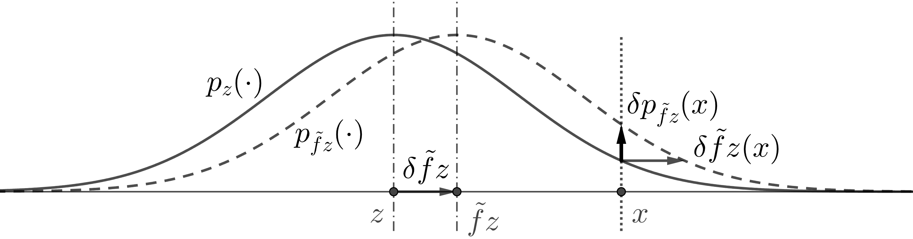
We explain this intuitively by figure 1. Let be distributed according to , then is obtained by first attach a density to each , then integrate over all . is obtained by first move to and then perform the same procedure. Hence, is first computing for each , then integrate over . Let
be the density of the noise centered at . So
Here in the middle expression is the horizontal shift of ’s level set previously located at . Since the entire Gaussian distribution is parallelly moved on the Euclidean space , so is constant for all . Then we can integrate over to get equation 7.
Using notation, Remark is equivalent to
where on the right is a function . Intuitively, this says that the left side equals to first compute for each , then integrate over . The integration on the left uses as dummy variable, which is convenient for the transfer operator formula above. But it does not involve a density for , so is not immediately ready for Monte-Carlo. The right integration is over and , which are easy to sample.
It is important that we differentiate only but not . In fact, our core intuitions are completely within one time step, and do not even involve . Hence, we can easily generalize to cases where is bad, for example, when is not bijective, or when is not hyperbolic: these are all difficult for deterministic systems.
2.4. Kernel-differentiation over finitely many steps
We use Remark to get integrated formulas for and its perturbation , which can be sampled by Monte-Carlo type algorithms. Note that here is fixed and does not depend on . This was previously known as the likelihood ratio method or the Monte-Carlo gradient method and was given in [37, 36, 17]. The magnitude of the integrand grows as after the centralization, where is the number of time steps.
Under assumption 1, for any (not necessarily positive) densities , any ,
Here the on the left is a dummy variable; whereas on the right is recursively defined by , so is a function of the dummy variables .
Remark.
The integrated formula is straightforward to compute by Monte-Carlo method. That is, for each , we generate random according to density , and i.i.d according to . Then we compute for this particular sample of . Note that the experiments for different should be either independent or decorrelated. Then the Monte-Carlo integration is simply
Almost surely according to . In this paper we shall use to indicate time steps, whereas labels different samples.
Proof.
Sequentially apply the definition of and , we get
| (8) |
Here in the last expression is a function of the dummy variables and . Roughly speaking, the dummy variable in the second expressions is .
Recursively apply equation 8 once, we have
Here , so is a function of the dummy variables , and . Keep applying equation 8 recursively to prove the lemma. ∎
[kernel-differentiation formula for ] Under assumption 1, then
Here is the differential of , is the independent distribution of ’s, and is a function of dummy variables .
Proof.
Note that is fixed, use equation 6, and let , we get
For each , first apply section 2.4 several times,
Here is a function of . Then apply Remark once,
Now is a function of . Then apply section 2.4 several times again,
Then sum over to prove the theorem. ∎
Note that subtracting any constant from and does not change the linear response. We prove a more detailed statement in a Remark. Hence, we can centralize , i.e. replacing by , where the constant
We sometimes centralize by subtracting . The centralization reduces the amplitude of the integrand, so the Monte-Carlo method converges faster: this is also a known result and was discussed in for example [18].
Proof.
First note that a density function on with bounded norm must have , since otherwise its integration can not be one.
Then notice that is a function of dummy variables , so we can first integrate
Since as . Here is the differential of the function , whereas indicates the integration. ∎
For the convenience of computer coding, we explicitly rewrite this theorem into centralized and time-inhomogeneous form, where , , and are different for each step. This is the setting for many applications, such as finitely-deep neural networks. The following proposition can be proved similarly to our previous proofs. Note that we can reuse a lot of data should we also care about the perturbation of the averaged for other layers .
In the following proposition, let be the observable function defined on the last layer of dynamics. Let be the pushforward measure given by the dynamics in equation 2, that is, defined recursively by ; Let be the independent but not necessarily identical distribution of ’s.
[centralized kernel-differentiation formula for of time-inhomogeneous systems] If and satisfy assumption 1 for all , then
Here .
2.5. Ergodic kernel-differentiation formula over infinitely many steps
For the perturbation of physical measures, the kernel-differentiation formula for can further take the form of long-time average on an orbit. This reduces the magnitude of the integrand so the convergence is faster. Here we can apply the ergodic theorem, forget details of initial distribution, and sample by points from one long orbit. Note that this subsection requires that the dynamics is time-homogeneous ( and are the same for each step) to invoke ergodic theorems.
Proof.
By assumption 2, we can start from , apply the perturbed dynamics many times, and would converge to .
By Remark, for any ,
Note that is invariant measure, so the expression
Passing to ,
Note that this is the correlation function between and . By Remark, . By assumption 2, the derivatives expressed by the above summations uniformly converge to the expression in the lemma. Hence, the limit equals . ∎
See 1.2
Remark.
Recall that is determined by the rate of decay of correlations, whereas is the number of averaging samples. Typically in numerics.
Proof.
Since is invariant for the dynamic , if , then is a stationary sequence, so we can apply Birkhoff’s ergodic theorem (the version for stationary sequences),
By substitution we have
Then we can rerun the proof after centralizing . ∎
2.6. Further generalizations
2.6.1. depends on and
Our pictorial intuition does not care whether depends on or . So we can generalize all of our results to the case
We write down these formulas without repeating proofs.
Equation 4 and equation 5 become
Section 2.4 becomes
Here and on the right are recursively defined by , . We also have the pointwise formula
Since now depends on via three ways, section 2.2 becomes
Here derivatives and refer to writing the density as . If does not depend on and , then we recover section 2.2. Remark becomes
Here
Remark becomes
Here is the distribution of ’s; is a function of dummy variables .
We still have free centralization for . So Remark and section 1.2 still hold accordingly, in particular, when the system is time-homogeneous and has physical measure , we still have
2.6.2. General random dynamical systems
For general random dynamical systems, at each step , we randomly select a map from a family of maps, denote this random map by , the dynamics is now
The selection of ’s are independent among different . It is not hard to see our pictorial intuition still applies, so our work can generalize to this case.
We can also formally transform this general case to the case in the previous subsubsection. To do so, define the deterministic map
where the expectation is with respect to the randomness of . Then the dynamic equals in distribution to
Hence the distribution of is completely determined by . Note that we still need to compute derivatives of the distribution of , or .
3. Foliated noise and perturbation
This section shows that the kernel-differentiation formulas are still correct for the case where the noise and are along a given foliation.
3.1. Preparation: measure notations, flotations, conditional densities
We assume that a neighborhood of the support of the physical measure can be foliated by a single chart: this basically means that we can partition the neighborhood by co-dimension- submanifolds. More specifically, this means that there is a family of co-dimension- submanifolds on , and a (we are not careful about the degree of differentiability) diffeomorphism between the neighborhood and an open set in , such that the image of is the -dimensional horizontal plane, . Each submanifold is called a ‘leaf’. An extension to the case where the neighborhood admits not a single chart, but a foliated atlas composed of many charts, is possible and we leave it to the future.
Under single-chart foliation, this section considers the system
The last equation just means that is a random variable depending on and , with details to be explained in the following paragraphs. The notation in the first equation relates to our previous notation when is a fixed diffeomorphism and .
We assume that and are parallel to . More specifically, for any in a small interval on and any ,
where is the leaf at . Note that we do not require being constrained by the foliation, so and can be on different leaves.
The measures considered in this section are not necessarily absolute continuous with respect to Lebesgue. So we should use another set of notations for measures. The transfer operator on measures is denoted by , more specifically, for any measure ,
We can disintegrate a measure into conditional measure on each leaf and the quotient measure on the set of . Since we have only one fixed foliation, we shall just omit the superscript . Here is a family of probability measures such that each ‘lives on’ . Moreover, the integration of any smooth observable can be written in two consecutive integrations,
We typically use to denote the measure of .
We assume that the random variable has a density function with respect to the Lebesgue measure on . That is, is the conditional density of . Then we can define the operator , which transfers , the measure of , to , the measure of . It transports measures only within each leaf, but not across different leaves, so the quotient measure is left unchanged. On the other hand, the density of the conditional measure is changed to
| (9) |
where is the Radon–Nikodym derivative with respect to the Lebesgue measure on . Note that does not necessarily have a density on . We have the double and triple integration formulas for the expectation of joint distribution
| (10) |
To summarize, we shall assume the following in this section.
Assumption 3.
Assume that a neighborhood of the support of the measures of interest is foliated by a family of leaves . For any , , . The density is on (but is singular with respect to ).
For the case of multiple steps, we shall denote the sequence of measures of by
where the limit is in the weak star sense, and is called the physical measure. We shall still make assumption 2. However, since the physical measure can be singular, it is more difficult to prove assumption 2 from some more basic assumptions; we did not find accurate references for this purpose.
3.2. Foliated kernel-differentiation in one step
We can see that the pictorial intuition in section 2.3 still makes sense on individual leaves. So it is not surprising that the main theorems are still effective. We shall first prove the formula on one leaf over one-step, which is the foliated version of sections 2.2 and Remark. Note that here one-step means to transfer the measure by , so the foliation is unchanged.
[local one-step kernel-differentiation on a leaf, comparable to section 2.2] Under assumptions 1 and 3, for any measure ,
Here , and the integrand is the derivative of with respect to in the direction . Here by default.
Remark.
Note that this differs from section 2.2 by a minus sign, since so taking derivaitives in gives a minus sign.
Proof.
By equation 9,
| (11) |
We give a formula for . By definition of and conditional densities, for any smooth observable function ,
Since preserves measure within each leaf, so the quotient measure is unchanged. Hence,
In short, we find that pushing-forward by commutes with taking conditions.
Substituting back to equation 11, we get
Then we can differentiate by and evaluate at to prove the lemma; note that at . ∎
[integrated one-step foliated kernel-differentiation, comparable to Remark] Under assumptions 1 and 3, for any fixed measure and any smooth observable ,
Remark.
See equation 10 for the probability notation which might help understanding.
Proof.
By the definition of conditional measure,
Since both and preserve the measure within each leaf, is not affected by . Further express the conditional measure by integrating the density, we get
| (12) |
Differentiate on both sides
Since every function in the integrand is bounded, we can move inside,
Apply section 3.2,
Then use equation 10 to transform triple integration to double integration. ∎
3.3. Foliated kernel-differentiation over finitely many steps
This subsection proves results for finitely many steps. Most proofs are similar to their counterparts in section 2.4, so we shall skip the proofs that are repetitive.
Remark.
Note that for the foliated case, the integration domain of depends on , so the multiple integration should first integrate with fixed.
[foliated kernel-differentiation formula for , comparable to Remark] Under assumptions 1 and 3, then
Proof.
Proof.
We first do the inner integrations for steps later than , which are all one. Hence, the left side of the equation,
Here is evaluated at by default. Then we can use Remark with set as a constant to prove the lemma. ∎
See 1.2
3.4. Foliated ergodic kernel-differentiation formula over infinitely many steps
This subsection is comparable to section 2.5 and states results for infinitely many steps. We shall skip the proofs since the ideas are the same and only the notations are a bit different.
[foliated kernel-differentiation formula for physical measures, comparable to section 2.5] Under assumptions 1, 2 and 3,
[orbitwise foliated kernel-differentiation formula for , comparable to section 1.2] Under assumptions 1, 2 and 3,
Here .
4. Kernel-differentiation algorithm
This section gives the procedure list of the algorithm, and demonstrates the algorithm on several examples. We no longer label the subscript , and can be the derivative evaluated at ; the dependence on should be clear from context. The codes used in this section are all at https://github.com/niangxiu/np.
4.1. Procedure lists
This subsection gives the procedure list of the kernel-differentiation algorithm for of a finite-time system, whose formula was derived in Remark. Then we give the procedure list for infinite-time system, whose formula was derived in section 1.2. The foliated cases have the same algorithm, and we only need to change to the suitable definition of .
First, we give algorithm for finite-time system. Here is the number of sample paths whose initial conditions are generated independently from (or , if the measure is singular and does not have a density). This algorithm requires that we already have a random number generator for and : this is typically easier for since we tend to use simple such as Gaussian; but we might ask for specific , which requires more advanced sampling tools.
Then we give the procedure list for the infinite-time case. Here is the number of preparation steps, during which the background measure is evolved, so that is distributed according to the physical measure . Here is the decorrelation step number, typically , where is the orbit length. Since here is given by the dynamic, we only need to sample the easier density .
From a utility point of view, the kernel-differentiation is an ‘adjoint’ algorithm. Since we do not compute the Jacobian matrix at all, so the most expensive operation per step is only computing and , so the cost for computing the linear response of the first parameter (i.e. a ) is cheaper than adjoint methods. On the other hand, the marginal cost for a new parameter in this algorithm is low, and it equals that of adjoint methods.
We remind readers of some useful formulas when we use Gaussian noise in . Let the mean be , the covariance matrix be , which is defined by . Then the density is
Hence we have
Typically we use normal Gaussian, so and , so we have
| (13) |
If we consider the co-dimension- foliation by planes , the above formula is still valid. For geometers, it might feel more comfortable to write together, which is just the directional derivative of the function defined on the subspace.
4.2. Numerical example: tent map with elevating center
We demonstrate the ergodic algorithm over infinitely many steps on the tent map. The dynamics is
In this subsection, we fix the observable
Previous linear response algorithms based on randomizing algorithms for deterministic systems, (such as fast response algorithm, path perturbation algorithm, divergence algorithm) do not work on this example. In fact, it is proved by Baladi that for the deterministic case (), linear response does not exist [4].
We shall demonstrate the kernel-differentiation algorithm on this example, and show that the noise case can give a useful approximate linear response to the deterministic case. In the following discussions, unless otherwise noted, the default values for the (hyper-)parameters are
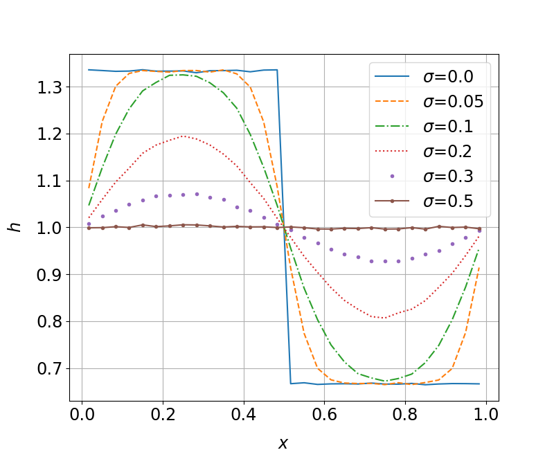
We first test the effect of adding noise on the physical measure. As shown in figure 2, the density converges to the deterministic case as . This and later numerical results indicate that we can wish to find some approximate ‘linear response’ for the deterministic system, which provides some useful information about the trends between the averaged observable and .
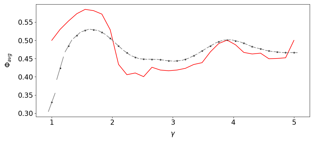
Then we run the kernel-differentiation algorithm to compute linear responses for different . This reveals the relation between and . As we can see, the algorithm gives an accurate linear response for the noised case. Moreover, the linear response in the noised case is an reasonable reflection of the observable-parameter relation of the deterministic case. Most importantly, the local min/max of the noised and deterministic cases tend to locate similarly. Hence, we can use the kernel-differentiation algorithm of the noised case to help optimizations of the deterministic case.
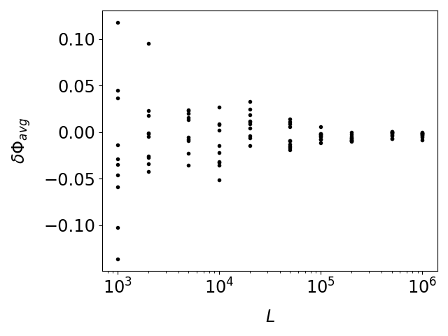
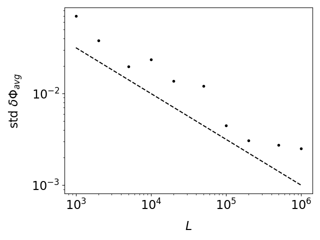
Then we show the convergence of the kernel-differentiation algorithm with respect to in figure 4. In particular, the standard deviation of the computed derivative is proportional to . This is the same as the classical Monte Carlo method for integrating probabilities, with being the number of samples. This is expected: since here we are given the dynamics, so our samples are canonically the points on a long orbit.
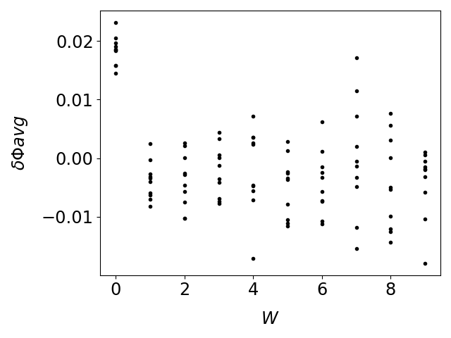
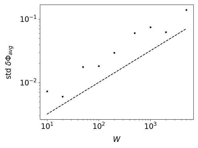
Figure 5 shows that the bias in the average derivative decreases as increases, but the standard deviation increases roughly like . Note that if we do not centralize , then the standard deviation would be like .
4.3. A chaotic neural network with foliated perturbations
4.3.1. Basic model
This subsection considers a chaotic neural network whose dynamic is deterministic, and the exact linear response does not provide useful information. Since the perturbation is foliated, we can add only a low-dimensional noise, which incur less errors. Then we use the kernel-differentiation algorithm to compute approximations of the linear response.
A main goal in design neural networks is to suppress gradient explosion, which is essentially the definition of chaos. However, even with modern architecture, there is no guarantee that gradient explosion (or chaos) can be precluded. Unlike stochastic backpropagation method, we do not perform propagation at all, so we are not hindered by gradient explosion. But we add extra noise at each layer, which introduces a (potentially large) systematic error.
The variables of interest are , , where , and the dynamic is
Here is the identity matrix, , and for ,
We set . The objective function is
There is a somewhat tight region for such that the system is chaotic: when , then is small so the Jacobian is small; when , then the points tend to be far from zero, so the derivative of is small, so the Jacobian is also small. Our choice gives roughly the most unstable network, and we roughly compare with the cost of the ensemble, or stochastic gradient, formula of the linear response, which is
Here is the backpropagation operator for covectors, which is the transpose of the is the Jacobian matrix . On average , , so the integrand’s size is about . This would require about samples (a sample is a realization of the 50-layer network) to reduce the sampling error to . That is not affordable.
Our model is modified from its original form in [7, 8]. In the original model, the entries of the weight matrix were randomly generated according to certain laws; as discussed in section 2.6.2, we can rewrite the random maps by an additive noise, then obtain exact solutions to the original problem. We can also further generalize this example to time-inhomogeneous cases.
Finally, we acknowledge that our neural network’s architecture is outdated, but modern architectures are not good tests for our algorithm. Because the backpropagation method does not work in chaos, current architectures typically avoid chaos. The kernel-differentiation method might help us to have more freedom in choosing architectures beyond the current ones.
4.3.2. Explicit foliated chart and artificial noise
We say the perturbation is foliated, which means that there is a fixed foliation such that for a small interval of , is always parallel to that foliation. The perturbation in this particular example is foliated, since for any ,
Hence, the vector field is invariant for an interval of , and the foliation is given by the streamlines of .
In fact, we can write down the explicit expression of a foliated chart, that is, change coordinate by , then the dynamic and the observable under the new coordinate is
Note that we can allow the chart to depend on . Also, the initial distribution is changed to
Now it is clear that is always in the direction of ; hence, we only need to add noise in this direction. We compute the linear response of the system
| (14) |
We shall compare with adding noise in all directions, with
Here is the identity matrix.
The foliated case has smaller noise added to the system, since equals summing i.i.d pieces of in orthogonal directions for times. Then we show that the two cases with noise have the same computational cost. As to be discussed in section 5.1, the computational cost is determined by the number of samples required, which is further determined by the magnitude of the integrand. To verify this, we check
where is the density on the 1-dimensional subspace, and is the density in all directions. By equation 13, and note that is constant, we want
This is indeed true, just notice that is the unit vector.
Note that now both and depends on due to the chart. Hence, the linear response has two more terms,
| (15) |
where the first term is given by section 1.2, and the other two terms are new. For the second term, since the integrand is constant, so the second term is ; if the integrand is not constant then we can still do Monte-Carlo sampling easily. For the third term, the expectation is just an abbreviation for the multiple integration in section 1.2. By definition,
so .
4.3.3. Numerical results
We use the kernel-differentiation method given in section 1.2 to compute the main term in equation 15, under two different noises: a noise in all directions, and a 1-dimensional noise along the direction of .
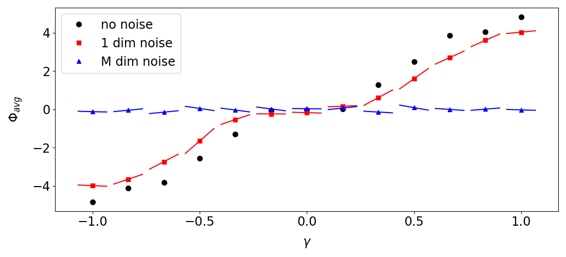
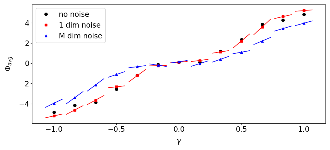
Figure 6 and figure 7 show the results of the kernel-differentiation algorithm on this example. The algorithm correctly computes the derivative of the problem with additive noises. The total time cost for running the algorithm on orbits to get a linear response, using a 1 GHz computer thread, is 3 seconds.
As we can see by comparing the two figures, the case with 1-dimensional noise is a better approximation of the deterministic case, which is what we are actually interested in. In particular, when , the -dimensional noise basically hides away any trend between the parameter and the averaged observable . In contrast, the 1-dimensional noise has a much smaller impact on the relation, and the derivative computed by the kernel differentiation method is more useful.
Also note that it is not free to decrease for the purpose of reducing the systematic error. As we can see by comparing the two figures, and as we shall discuss in section 5.1, small would increase the sampling error, which further requires more samples to take down, and this increases the cost. So adding low-dimensional noise, when the perturbation is foliated, has a unique advantage of reducing the approximation error to deterministic case.
5. Discussions
The kernel-differentiation algorithm is robust, does not have systematic error, has low cost per step, and is not cursed by dimensionality. But there is a caveat: when the noise is small, we need many data for the Monte-Carlo method to converge. Hence we can not expect to use the small limit to get an easy approximation of the linear response for deterministic systems.
In this section, we first give a rough cost-error estimation of the problem, and estimate the number of samples and desirable noise intensity . Then we discuss how to potentially reduce the cost by further combining with the fast response algorithm, which was developed for deterministic linear responses.
5.1. A rough cost-error estimation
When the problem is intrinsically random, the scale of noise has been fixed. For this case, there are two sources of error. The first is due to using a finite decorrelation step number ; this error is for some . The second is the sampling error due to using a finite number of samples. Assume we use Gaussian noise, since we are averaging a large integrand to get a small number, we can approximate the standard deviation of the integrand by its absolute value. The integrand is the sum of copies of , so the size is roughly . So the sampling error is , where is the number of samples. Together we have the total error
This gives us a relation among , and , where is proportional to the overall cost. In practice, we typically set the two errors be roughly equal, which gives an extra relation for us to eliminate and obtain the cost-error relation
This is rather typical for Monte-Carlo method. But the problem is that cost can be large for small .
On the other hand, if we use random system to approximate deterministic systems, then we can have the choice on the noise scale . Now each step further incurs an approximation error on the measure. This error decays but accumulates, and the total error on the physical measure is , which can be quite large compared to the one-step error . Hence, if we are interested in the trend between and for a certain stepsize (this is typically known from the practical problem), then the error in the linear response is . Together we have the total error
| (16) |
Again, in practice we want the three errors to be roughly equal, which shall prescribe the size of ,
Since can be small, this cost can be much larger than just , which is already a high cost.
Finally, we acknowledge that our estimation is very inaccurate, but the point we make is solid, that is, the small noise limit is numerically expensive to achieve.
5.2. A potential program to unify three linear response formulas
We sketch a potential program on how to further reduce the cost/error of computing approximate linear response of non-hyperbolic deterministic systems. As is known, non-hyperbolic systems do not typically have linear responses, so we must mollify, and in this paper we choose to mollify by adding noise in the phase space during each time step. But as we see in the last subsection, adding a big noise increases the noise error, the third term in equation 16; whereas small noise increases the sampling error, the second term in equation 16.
There are cases with special structures, and we have specific tools which could give a good approximate linear response, in terms of reflecting the parameter-observable relation. When the system has a foliated structure, this papers shows that we can add low-dimensional noise. When the unstable dimension is low, computing only the shadowing or stable part of the linear response may be a good approximation (see [28]).
For the more general situation, a plausible solution is to add a big but local noise, only at locations where the hyperbolicity is bad. The benefit of this program is that, if the singularity set is low-dimensional, then the area where we add big noise is small, and the noise error is small. For continuous-time case there seems to be an easy choice: we can let the noise scale be reverse proportional to the flow vector length. This should at least solve the singular hyperbolic flow cases [40, 41], where the bad points coincide with zero velocity. But for discrete-time case it can be difficult to find a natural criteria which is easy to compute.
In terms of the formulas, we use the kernel-differentiation formula (the generalized version in section 2.6) where the noise is big, so the sampling error is also small. Where the noise is small, we use the fast-response algorithm, which is efficient regardless of noise scale, but requires hyperbolicity.
This program hinges on the assumption that the singularity set is small or low-dimensional. It also requires us to invent more techniques. For example, we need a formula which transfers information from the kernel-differentiation formula to the fast response formulas. For example, the equivariant divergence formula, in its original form, requires information from the infinite past and future [30]. But we can rerun the proof and restrict the time dependence to finite time; this requires extra information on the interface, such as the derivative of the conditional measure and the divergence of the holonomy map. These information should and could be provided by the kernel-differentiation formula.
Historically, there are three famous linear response formulas. The path-perturbation formula does not work for chaos; the divergence formula is likely to be cursed by dimensionality; the kernel-differentiation formula is expensive for small noise limit. The fast response formula combines the path-perturbation and the divergence formula, it is a function (not a distribution) so can be sampled; it is neither affected by chaos or high-dimension, but is rigid on hyperbolicity. In the future, besides trying to test above methods on specific tasks, we should also try to combine all three formulas together into one, which might provide the best approximate linear responses with highest efficiency.
Acknowledgements
The author is in great debt to Stefano Galatolo, Yang Liu, Caroline Wormell, Wael Bahsoun, and Gary Froyland for helpful discussions.
Data availability statement
The code used in this manuscript is at https://github.com/niangxiu/kd. There is no other associated data.
References
- [1] F. Antown, G. Froyland, and S. Galatolo. Optimal linear response for markov hilbert–schmidt integral operators and stochastic dynamical systems. Journal of Nonlinear Science, 32, 12 2022.
- [2] W. Bahsoun, S. Galatolo, I. Nisoli, and X. Niu. A rigorous computational approach to linear response. Nonlinearity, 31:1073–1109, 2018.
- [3] W. Bahsoun, M. Ruziboev, and B. Saussol. Linear response for random dynamical systems. Advances in Mathematics, 364:107011, 4 2020.
- [4] V. Baladi. On the susceptibility function of piecewise expanding interval maps. Communications in Mathematical Physics, 275:839–859, 8 2007.
- [5] V. Baladi. The quest for the ultimate anisotropic banach space. Journal of Statistical Physics, 166:525–557, 2017.
- [6] R. Bowen and D. Ruelle. The ergodic theory of axiom a flows. Inventiones Mathematicae, 29:181–202, 1975.
- [7] B. Cessac and J. A. Sepulchre. Stable resonances and signal propagation in a chaotic network of coupled units. Physical Review E, 70:056111, 11 2004.
- [8] B. Cessac and J. A. Sepulchre. Transmitting a signal by amplitude modulation in a chaotic network. Chaos: An Interdisciplinary Journal of Nonlinear Science, 16:013104, 3 2006.
- [9] D. Dolgopyat. On differentiability of srb states for partially hyperbolic systems. Inventiones Mathematicae, 155:389–449, 2004.
- [10] D. Dragičević, P. Giulietti, and J. Sedro. Quenched linear response for smooth expanding on average cocycles. Communications in Mathematical Physics, 399:423–452, 4 2023.
- [11] R. Durrett. Probability: Theory and Examples. Cambridge University Press, 4th edition edition, 8 2010.
- [12] G. L. Eyink, T. W. N. Haine, and D. J. Lea. Ruelle’s linear response formula, ensemble adjoint schemes and lévy flights. Nonlinearity, 17:1867–1889, 2004.
- [13] G. Froyland, D. Giannakis, B. R. Lintner, M. Pike, and J. Slawinska. Spectral analysis of climate dynamics with operator-theoretic approaches. Nature Communications, 12:6570, 11 2021.
- [14] S. Galatolo and P. Giulietti. A linear response for dynamical systems with additive noise. Nonlinearity, 32:2269–2301, 6 2019.
- [15] S. Galatolo and I. Nisoli. An elementary approach to rigorous approximation of invariant measures. SIAM Journal on Applied Dynamical Systems, 13:958–985, 2014.
- [16] M. Ghil and V. Lucarini. The physics of climate variability and climate change. Reviews of Modern Physics, 92:035002, 7 2020.
- [17] P. W. Glynn. Likelihood ratio gradient estimation for stochastic systems. Communications of the ACM, 33:75–84, 10 1990.
- [18] P. W. Glynn and M. Olvera-Cravioto. Likelihood ratio gradient estimation for steady-state parameters. Stochastic Systems, 9:83–100, 6 2019.
- [19] S. Gouëzel and C. Liverani. Compact locally maximal hyperbolic sets for smooth maps: Fine statistical properties. Journal of Differential Geometry, 79:433–477, 2008.
- [20] M. S. Gutiérrez and V. Lucarini. Response and sensitivity using markov chains. Journal of Statistical Physics, 179:1572–1593, 2020.
- [21] M. Hairer and A. J. Majda. A simple framework to justify linear response theory. Nonlinearity, 23:909–922, 4 2010.
- [22] K. He, X. Zhang, S. Ren, and J. Sun. Deep residual learning for image recognition. In IEEE conference on computer vision and pattern recognition, pages 1–12, 2016.
- [23] A. Jameson. Aerodynamic design via control theory. Journal of Scientific Computing, 3:233–260, 1988. Firstintroduce adjoint method into aerodynamic design.
- [24] M. Jiang. Differentiating potential functions of srb measures on hyperbolic attractors. Ergodic Theory and Dynamical Systems, 32:1350–1369, 2012.
- [25] D. J. Lea, M. R. Allen, and T. W. N. Haine. Sensitivity analysis of the climate of a chaotic system. Tellus A: Dynamic Meteorology and Oceanography, 52:523–532, 2000.
- [26] V. Lucarini, F. Ragone, and F. Lunkeit. Predicting climate change using response theory: Global averages and spatial patterns. Journal of Statistical Physics, 166:1036–1064, 2017.
- [27] A. Ni. Hyperbolicity, shadowing directions and sensitivity analysis of a turbulent three-dimensional flow. Journal of Fluid Mechanics, 863:644–669, 2019.
- [28] A. Ni. Approximating linear response by nonintrusive shadowing algorithms. SIAM J. Numer. Anal., 59:2843–2865, 2021.
- [29] A. Ni. Backpropagation in hyperbolic chaos via adjoint shadowing. Nonlinearity, 37:035009, 3 2024.
- [30] A. Ni and Y. Tong. Recursive divergence formulas for perturbing unstable transfer operators and physical measures. Journal of Statistical Physics, 190:126, 7 2023.
- [31] A. Ni and Y. Tong. Equivariant divergence formula for hyperbolic chaotic flows. Journal of Statistical Physics, 191:118, 9 2024.
- [32] R. Pascanu, T. Mikolov, and Y. Bengio. On the difficulty of training recurrent neural networks. International conference on machine learning, pages 1310–1318, 2013.
- [33] P. Plecháč, G. Stoltz, and T. Wang. Convergence of the likelihood ratio method for linear response of non-equilibrium stationary states. ESAIM: Mathematical Modelling and Numerical Analysis, 55:S593–S623, 2021.
- [34] P. Plecháč, G. Stoltz, and T. Wang. Martingale product estimators for sensitivity analysis in computational statistical physics. IMA Journal of Numerical Analysis, 43:3430–3477, 11 2023.
- [35] M. Pollicott and O. Jenkinson. Computing invariant densities and metric entropy. Communications in Mathematical Physics, 211:687–703, 2000.
- [36] M. I. Reiman and A. Weiss. Sensitivity analysis for simulations via likelihood ratios. Operations Research, 37:830–844, 10 1989.
- [37] R. Y. Rubinstein. Sensitivity analysis and performance extrapolation for computer simulation models. Operations Research, 37:72–81, 2 1989.
- [38] D. Ruelle. A measure associated with axiom-a attractors. American Journal of Mathematics, 98:619, 1976.
- [39] D. Ruelle. Differentiation of srb states. Commun. Math. Phys, 187:227–241, 1997.
- [40] M. Viana. What’s new on lorenz strange attractors? The Mathematical Intelligencer, 22:6–19, 6 2000.
- [41] X. Wen and L. Wen. No-shadowing for singular hyperbolic sets with a singularity. Discrete and Continuous Dynamical Systems- Series A, 40:6043–6059, 10 2020.
- [42] C. L. Wormell and G. A. Gottwald. Linear response for macroscopic observables in high-dimensional systems. Chaos, 29, 2019.
- [43] L.-S. Young. What are srb measures, and which dynamical systems have them? Journal of Statistical Physics, 108:733–754, 2002.