Error Exponents of Optimum Decoding for the Interference Channel
Raul H. Etkin†,
Neri Merhav‡,
and Erik Ordentlich†,
raul.etkin@hp.com, merhav@ee.technion.ac.il, erik.ordentlich@hp.com
†R. Etkin and E. Ordentlich are with Hewlett-Packard Laboratories, Palo Alto, CA 94304, USA.‡N. Merhav is with Technion - Israel Institute of Technology, Haifa 32000, Israel. Part of this work was done while N. Merhav was visiting Hewlett–Packard Laboratories
in the Summers of 2007 and 2008.
Abstract
Exponential error bounds for the finite–alphabet interference channel (IFC) with two transmitter–receiver pairs, are investigated under the random coding regime. Our focus is on optimum decoding, as opposed to
heuristic decoding rules that have been used in previous works, like joint typicality
decoding, decoding based on interference cancellation, and decoding that considers the
interference as additional noise. Indeed, the fact that the actual
interfering signal is a codeword and not an i.i.d. noise process complicates the application of conventional techniques to the performance analysis of the optimum decoder.
Using analytical tools rooted in
statistical physics, we derive a single letter expression
for error exponents achievable under optimum decoding
and demonstrate strict improvement over error exponents
obtainable using suboptimal decoding rules, but which are amenable
to more conventional analysis.
Index Terms:
Error exponent region, large deviations, method of types, statistical physics.
I Introduction
The -user interference channel (IFC) models the communication
between transmitter-receiver pairs, wherein each receiver
must
decode its corresponding transmitter’s message from a signal that is corrupted by interference from the
other transmitters, in addition to channel noise. The information
theoretic analysis of the IFC was initiated over 30 year ago
and has recently witnessed a resurgence of interest, motivated by new
potential applications, such as wireless communication over
unregulated spectrum.
Previous work on the IFC has focused on obtaining inner and outer
bounds to the capacity region for memoryless interference and noise,
with a precise characterization of the capacity region remaining
elusive for most channels, even for users. The best known
inner bound for the IFC is the Han-Kobayashi (HK) region, established
in [1]. It has been found to be tight in certain special cases
([1, 2]), and recently was found to be tight to within 1 bit for the
two user Gaussian IFC [3]. No achievable rates that lie outside the HK
region are known for any IFC with users.
Our aim in this paper is to extend the study of achievable schemes to
the analysis of error exponents, or exponential rates of decay of
error probabilities, that are attainable as a function of user rates.
To our knowledge, there has been no prior treatment of error exponents
for the IFC. In particular, the error bounds underlying the achievability results
in [1] yield vanishing error exponents (though still decaying
error probability) at all rates.
The notion of an error exponent region, or a set of achievable
exponential rates of decay in the error probabilities for different
users at a given operating rate-tuple in a multi-user communication
network, was formalized recently in [4], and studied therein
for Gaussian multiple access and broadcast channels.
Our main result, presented in Section IV, is a single letter
characterization of an achievable error exponent region, as a function
of user rates, for the user finite alphabet, memoryless
interference channel.
The region is derived by bounding the average
error probability of random codebooks comprised of i.i.d. codewords
uniformly distributed over a type class, under maximum likelihood (ML)
decoding at each user. Unlike the single user setting, in this case,
the effective channel determining each receiver’s ML
decoding rule is induced both by the noise and the interfering
user’s codebook. Our focus on optimal decoding is a departure from
the conventional achievability arguments in [1] and elsewhere,
which are based on joint-typicality decoding, with restrictions on the
decoder to “treat interference as noise” or to “decode the
interference” in part or in whole. However, in this work, we confine our analysis to
codebook ensembles that are simpler than the superposition codebooks of [1].
The analysis of the probability of decoding error under optimal decoding
is complicated due to correlations induced by the interfering signal.
Usual methods for bounding the probability of error based on
Jensen’s inequality and
other related inequalities (see, e.g., (8) below)
fail to give good results.
Our bounding approach combines some of the
classical information theoretic approaches of [5]
and [6] with an analytical technique from statistical
physics that was applied recently to the study of single user channels
in [7, 8]. More specifically,
as in [5], we use auxiliary parameters and
to get an upper bound on the average probability of decoding
error under ML decoding, which we then bound using the method of types
[6]. Key in our derivation is the use of distance enumerators
in the spirit of [7] and [8],
which allows us to avoid using Jensen’s
inequality in some steps, and allows us to maintain exponential
tightness in other inequalities by applying them to only
polynomially few terms (as opposed to exponentially many)
in certain sums that bound the probability of decoding error.
It should be emphasized, in this context, that the use of this technique was pivotal to
our results. Our earlier attempts, that were based on more ‘traditional’
tools, failed to provide meaningful results. In fact, they all turned
out to be inferior to some trivial bounds.
The paper is organized as follows. The notation, various definitions, and the
channel model assumed throughout the paper are detailed in
Section II. In Section III,
we derive an “easy”
set of attainable error exponents which
we shall treat as a benchmark for the exponents of the main section,
Section IV. The “easy” exponents are obtained by simple
extensions
to the interference channel of existing error exponent
results for single user and multiple access channels, based on random constant
composition codebooks and suboptimal decoders.
Then, in Section IV, we derive another set of attainable
exponents by analyzing ML decoding for the
channel induced by the interfering codebook. In Section V,
we show that the minimizations required to evaluate the new error exponents can be
written as convex optimization problems, and, as a result, can be solved efficiently.
We follow this up in
Section VI with a numerical comparison
of the new exponents with the baseline exponents of Section III for a simple
IFC. These numerical results demonstrate that the new exponents are never worse (at least for the chosen channel and parameters) and, for most rates, strictly improve over the baseline exponents.
An earlier version of this work was presented in [9].
II Notation, Definitions, and Channel Model
Unless otherwise stated, we use lowercase and uppercase letters for scalars, boldface
lowercase letters for vectors, uppercase (boldface) letters for random variables (vectors),
and calligraphic letters for sets. For example, is a scalar, is a vector,
is a random variable, is a random vector, and is a set. For a real number we shall, on occasion, let denote .
Also, we use to denote natural logarithm, to denote
expectation, and Pr to denote probability.
For independent random variables and
distributed according to ,
, we denote the conditional expectation operator
as for any function . All information quantities (entropy, mutual information, etc.) and rates are in nats.
Finally, we use , , etc., to denote equality or inequality to the first order in the exponent, i.e. ; .
The empirical probability mass function of the finite alphabet sequence
with alphabet
is denoted as the vector , where each
is the relative frequency of along . The type class associated
with an empirical probability mass function , which will be denoted
by , is the set of all –vectors whose empirical
probability mass function is equal to .
Similar conventions will apply to pairs and triples of vectors
of length , which are defined over the corresponding
product alphabets. Information measures pertaining to empirical distributions will be denoted using the standard notational conventions, except that we use “” as well as subscripts that indicate the sequences from which these empirical distributions were extracted. For example, we write
and to denote the conditional entropy of given and the mutual information between and , respectively, computed with respect to the empirical distribution . We denote the relative entropy or Kullback-Leibler divergence between distributions and as , and we write for the conditional relative entropy between conditional distributions and conditioned on , which is defined as .
We continue with a formal description of the two–user IFC setting.
Let , ,
denote the channel input signals of the two transmitters, and let
be the corresponding
channel outputs received by decoders 1 and 2, where and denote the input and output alphabets, and which we assume
to be finite. Each (random) output symbol pair
is assumed to be conditionally independent of all other outputs, and
all input symbols, given the two corresponding (random) input symbols
, and the corresponding conditional probability
is assumed to be constant from symbol to symbol. An
code for the IFC consists of pairs of encoding and
decoding functions, and , respectively,
where ,
, and
, . The
performance of the code is characterized by a pair of error
probabilities , , where
and is the random output when
user transmits ,
assuming the messages are uniformly distributed on the
sets of indices , . The per
user error probabilities depend on the channel only through the
marginal conditional distributions of the channel outputs given the
corresponding channel input pairs. We shall denote these conditional
distributions as .
A pair of error exponents is attainable at a rate pair if there is a sequence of codes
satisfying for .
The set of all attainable error exponents at comprises
the error exponent region at and we shall denote it as . The main result of this paper is a single letter
characterization of a non–trivial subset of for
each .
III Background
In this section, we present achievable error exponents for the interference channel which are based on known results of error exponents for single user and multiple access channels (MAC) for fixed composition codebooks [12, 13, 11]. These exponents will be used as a baseline for comparing the performance of the error exponents that we derive in Section IV.
In the following, we will focus on the error performance of user 1, and as a result, all explanations and expressions will be specialized to receiver 1. Similar expressions also hold for user 2 with the exchange of indices .
A possibly suboptimal decoder for the interference channel can be obtained from a given multiple access channel decoder by simply ignoring the decoded message of the interfering transmitter. For example, following [13], we can use a minimum entropy decoder that for a given received vector at receiver computes
and throws away .
It follows from [13] that for random codebooks of fixed composition , the average probability of decoding both messages in error, where the averaging is done over the random choice of codebooks, satisfies:
where
with .
In addition, the average probability of decoding the message of the interfering transmitter correctly but the message of the desired transmitter incorrectly satisfies:
where
Therefore, the overall average error performance of this MAC decoder in the IFC satisfies:
A second suboptimal decoder that leads to tractable error performance bounds is the single user maximum mutual information decoder (which in this case coincides with the minimum entropy decoder):
In this case, standard application of the method of types [11] leads to the following bound on the average error probability under random fixed composition codebooks of types :
where
We can choose the better decoder between these two, that leads to the better error performance. Therefore, we obtain that
(1)
is an achievable error exponent at receiver 1, with an analogous exponent following for receiver 2.
IV Main Result
Our main contribution is stated in the following theorem,
which presents a new error exponent region
for the discrete memoryless two–user IFC.
While the full proof appears in Appendix A, we also provide
a proof outline below, to give an idea of the main steps.
Theorem 1
For a discrete memoryless two-user IFC as defined in Section I, for a family of block codes of rates and a decoding error probability for user 1 satisfying
(2)
can be achieved as the block length
of the codes goes to infinity, where the
error exponent is given by
(3)
where
(4)
(5)
with
and
(6)
(7)
where is the probability simplex in . In the bound (2), can be chosen to maximize the error exponent .
In eqs. (2), (3), (6), and (7), and are probability distributions defined over the alphabets and respectively.
Expressions for the error probability and error exponent equivalent to (2) and (3) can be stated for the receiver of user 2 by replacing , , and in all the expressions. By varying and over all probability distributions in and respectively, we obtain the error exponent region for fixed rates and .
Remark 1
A lower bound to is
derived in Appendix B (cf. equation (B.4)) that is closer in form to the
expressions underlying the benchmark exponent presented
above. In particular, this lower bound allows us to establish
analytically (see Appendix B) that at (and for
sufficiently small ). Numerical computations, as presented in Section VI,
indicate that this inequality can be strict.
A second application of the lower bound (B.4) is to determine the set
of rate pairs for which . We show in Appendix B
that this region includes
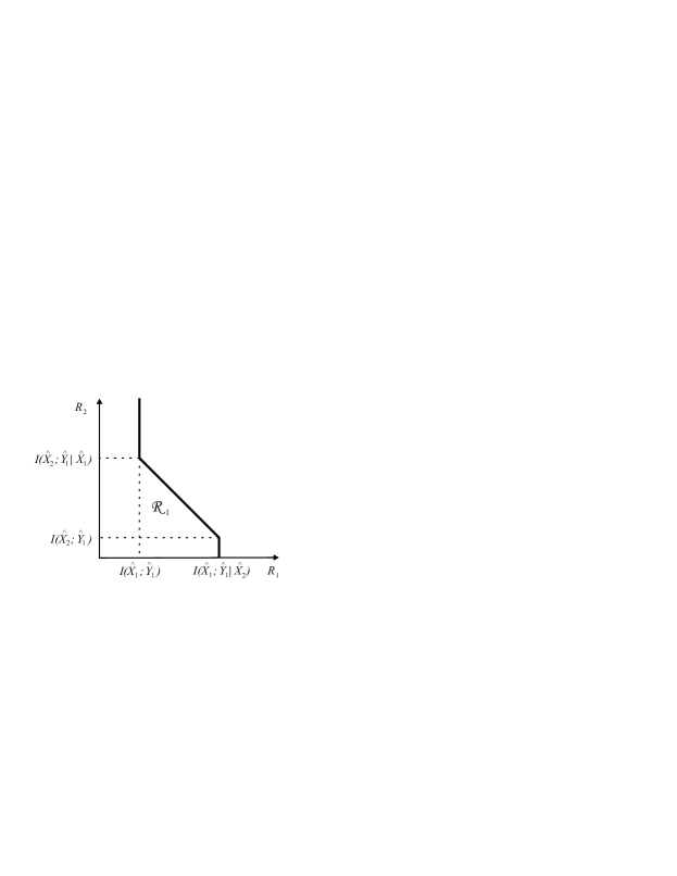
with an analogous region following for the set where (see Fig. 1).
Figure 1: Rate region where .
Furthermore, it is shown in [11] that the error exponent
achievable for user no. 1 with optimal decoding and random fixed composition codebooks
is zero outside the closure of the region . This result, together with our contribution
characterize the rate region where the attainable exponents with random constant composition codebooks are positive. Finally, it can be shown that this region is contained in the HK region [11].
Remark 2
Theorem 1 presents an asymptotic upper bound on the average probability of decoding error for fixed composition codebooks, where the averaging is done over the random choice of codebooks. It is straightforward to show (see, e.g., [4]) that there exists a specific (i.e. non-random) sequence of fixed composition codebooks of increasing block length for which the same asymptotic error performance can be achieved.
Proof Outline.
For non–negative reals and ,
the following inequality [5, Problem 4.15(f)] will be frequently used:
(8)
For a given block length , we generate the codebook of user by choosing sequences of length independently and uniformly over all the sequences of length and type in . Note that have rational entries with denominator . We will write to denote the -th codeword of user .
For a given channel output , the best decoding rule to minimize the probability of error in decoding the message of user 1 is ML decoding, which consists of picking the message which maximizes . Letting
(9)
be the “average” channel observed at receiver 1, where the averaging is done over the codewords of user 2 in , the decoding error probability at receiver 1 for transmitted codeword and codebooks and is given by:
(10)
With the introduction of the average channel (9), and the use of two auxiliary parameters , we can follow the approach of [5] to bound the conditional probability of decoding error . Taking expectation over the random choice of codebooks and we obtain an average error probability:
(11)
where we used Jensen’s inequality to move the second expectation
inside .
Equation (11) is hard to handle, mainly due to the correlation introduced by between the two factors inside the outer expectation. Furthermore, the evaluation of the inner expectations over are complicated due to the powers and affecting . Bounding methods based on Jensen’s inequality and
(8)
fail to give good results due to the loss of exponential tightness.
We proceed with a refined bounding technique based on the method of types inspired by [7]. While in this approach we still use (8), we use it to bound sums with a number of terms that only grows polynomially with , and as a result, exponential tightness is preserved.
Since the channel is memoryless,
(12)
where we used to denote the number of codewords in such that have empirical distribution . We also used to denote expectation with respect to the distribution .
Replacing (12) in (11) and using (8)
three times, we obtain:
(13)
where we used and to shorten the expression.
We next consider the bounding of
(14)
and note that and are formed by sums of an exponentially large number of indicator functions, each of which takes value 1 with exponentially small probability. These sums concentrate around their means, which show different behavior depending on how the number of terms in the sum () compares to the probability of each of the indicator functions taking value 1 (depending on the case considered, these probabilities take the form , , or ). Whenever one of the factors in (14) concentrates around its mean it behaves as a constant, and hence is uncorrelated with the remaining factor. As a result, the correlation between the two factors of (14), which complicates the analysis, can be circumvented. We give the details of this part of the derivation in Appendix A, but note here that the resulting bound on depends on
only through a factor . Therefore, the innermost sum in (13) can be evaluated by counting the number of vectors that have empirical types and . Note that this count can only be positive for . This count is approximately equal to to first order in the exponent. Furthermore, the sums over and in (13) have a number of terms that only grows polynomially with . Therefore, to first order, the exponential growth rate of (13) equals the maximum exponential growth rate of the argument of the outer two sums, where the maximization is performed over the distributions and which are rational, with denominator . We can further upper bound the probability of error by enlarging the optimization region, maximizing over any probability distributions .
V Convex Optimization Issues
In order to get a valid evaluation of ,
for any given satisfying the
constraints of the outer maximization, we need to
accurately solve the inner minimization problems. A brute
force search may not give accurate enough results in reasonable time.
As will be shown below, the first minimization problem in
(3) is a convex problem, and as a result, it that
can be solved efficiently. In addition, convexity allows to
lower bound the objective function by its supporting hyperplane,
which in turn, allows to get a reliable111In our
implementation we solve the original convex optimization
problem using the MATLAB function fmincon. lower
bound through the solution of a linear program.
The second minimization problem is not convex due to the
non–convex constraint .
If we remove this constraint, it will be later shown that
we obtain a convex problem that can be solved efficiently.
There are two possible situations:
The first situation occurs when the optimal solution to the modified problem
satisfies : in this case,
the solution to the modified problem is also a solution to the
original problem.
The second situation is when the optimal solution to the modified problem
satisfies :
in this case, a solution to the original problem must satisfy
. We prove this statement by contradiction.
Let be the optimal solution to the modified problem, and be
an optimal solution to the original problem.
Now assume conversely, that there is no
that satisfies . With this assumption, we have
that at , . Let
. Note that is a convex set
and . Due to the continuity of
, the
straight line in that joins and
must pass through an intermediate point , , that satisfies
. Let be the objective function
of the second minimization problem in (3), restricted to
. It will be shown later that , restricted to this
domain, is a convex function. By hypothesis, and
we have . On the other hand,
from the convexity of , restricted to , we have
and we get a contradiction. Therefore, it follows that there is a solution to
the original problem that satisfies .
Let be the objective function of the first minimization
problem in (3). First, we note that satisfies the
constraints of the first minimization problem since they are less restrictive
than the constraints of the second minimization problem in
(3). We next prove that . As a result, the
optimal solution of the first minimization problem satisfies
, and we do not need to know
to evaluate the argument of the maximization in
(3). Using the fact that at ,
, we have:
(15)
where we used the identity
in the second equality.
In summary, if the solution to the second minimization problem in
(3), without the constraint on , satisfies
, then the first minimization problem in
(3) dominates the expression. Otherwise, the solution to the
second minimization problem in (3) without the constraint
, equals the solution to the second
minimization problem with this constraint.
It remains to show that the objective functions of the minimization problems
in (3), , , restricted to the
domain , are convex functions.
Since the sum of convex functions is convex, to prove the convexity of
on , we only need to prove that the different
terms of
(16)
are convex within .
First, we have that
is linear in and therefore convex. Also, we have that
is convex for fixed due to the concavity of
.
In addition, can be written as
. Let for
any , such that
and . We have that and . The convexity of
for fixed follows from the
convexity of in the pair :
we note that it is the maximum of two convex functions, and therefore convex.
The convexity of each of the individual functions follows from the convexity of
for fixed , , which can be proved along
the same lines as (LABEL:eqn:convexI).
Each of the arguments of the can be shown to be the sum
of convex functions for fixed and , using a
similar argument as the one used to prove (LABEL:eqn:convexI). Since the
maximum of convex functions is convex, the convexity of restricted to
follows.
Using similar arguments, it is easy to show that
is convex in .
VI Numerical Results
In this section, we present a numerical example to show the performance of the error exponent region introduced in Theorem 1. We use as a baseline for comparison the error exponent region of Section III, which is obtained with minor modifications from known results for single user and multiple access channels.
We present results for the binary Z-channel model:
, , where , , is multiplication, and is modulo 2 addition. This is a modified version of the binary erasure IFC studied in [10], where we add noise to the received signal of user 1. In the results presented here, we fix .
The boundary of the error exponent region is a surface in four dimensions . This surface can be obtained parametrically by computing as a function of , by optimizing over and in (3) and in the corresponding expression for . The parameterization of in terms of , allows the study of the error performance as a function of the parameters that directly influence it.
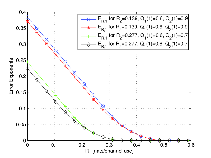
Figure 2: Error exponents as a function of for two different values of and fixed choices . All the rates are in nats.
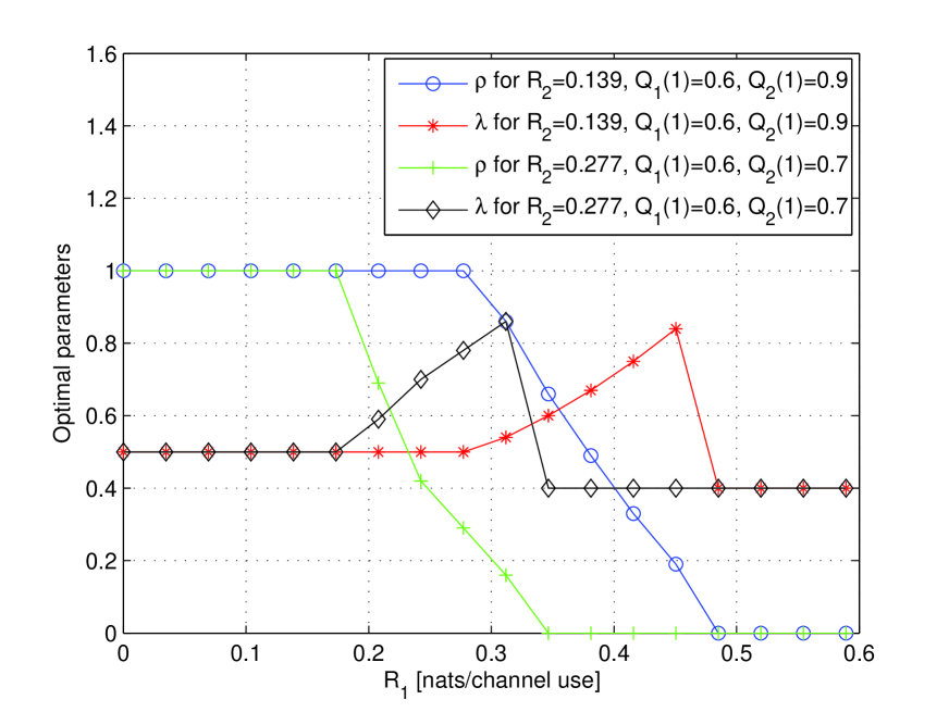
Figure 3: Optimal parameters and for the curves of Fig. 2. All the rates are in nats.
Fig. 2 shows that the error exponents under optimal decoding derived in this paper can be strictly better than the baseline error exponents of Section III. This suggests that the inequality obtained in Appendix B for can be strict. In addition, in all the plots that we computed for the Z-channel for different values of and we were not able to find a single case where the baseline exponent was larger than .
We see that the curves of () for fixed have a linear part for below a critical value (), and a curvy part for () (note that the critical values depend on the parameters and ). Figure 3 shows the optimal parameters and for the curves shown in Fig. 2 for and nats/channel use. We see that for the linear part of the curves and are optimal, while for the curvy part (i.e. ) the optimal decreases to 0 and the optimal increases towards 1. For in the interval the gap between the and curves remains constant as both curves are lines with slope , and this gap is equal to the gap at . In general, any gap between and at will remain constant in the interval where both curves have slope . We also note since the optimal parameters and vary for different rates, these parameters are indeed active, i.e. they have influence on the resulting error exponent.
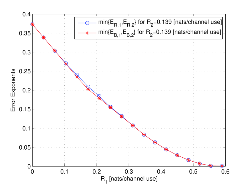
The curves of Fig. 2 are obtained for fixed choices of and , which are the distributions used to generate the random fixed composition codebooks. As and vary in the probability simplex , we obtain the four-dimensional error exponent region . In order to obtain a two-dimensional plot of the region, we consider a projection: we fix varying and plot the maximum value over and in the error exponent region of . This corresponds to choosing and in order to maximize the error exponent simultaneously achievable for both users. Figure 4 shows this projection for and nats/channel use, where, for reference, we included the corresponding curves for the error exponents of Section III.
Figure 4: Maximum error exponent simultaneously achievable for both users for fixed as a function of .
For the noiseless binary channel of user 2, , and as a result, decreases with increasing for . On the other hand, because of the multiplication between and in the received signal , increasing results in less interference for user 1, and a larger value of . It follows that there is a direct trade-off between and through the choice of , and whenever is maximized, . Therefore, in the curve of Fig. 4, .
From the plots of Figs. 2 and 4, we see that the error exponents obtained from Theorem 1 sometimes outperform and are never worse than the baseline error exponents of Section III.
It is easy to see that the optimum decoder for user 1
picks the message () that
maximizes , where
and .
Applying Gallager’s general upper bound to the “channel”
,
we have for user no. 1:
(A.1)
where and are arbitrary parameters to be
optimized in the sequel.
Thus, the average error probability
is upper bounded by the expectation of the above
w.r.t. the ensemble of codes of both users.
Let us take the expectation
w.r.t. the ensemble of user 1 first, and we denote this expectation
operator by . Since the codewords of user 1 are
independent, the expectation of the summand in the sum above
is given by the product of expectations, namely, the product of
(A.2)
and
Now, let
denote the number of codewords
that form a joint empirical PMF
together with a given and .
Then, using (8), can be bounded by
(A.3)
where
is the
single–letter transition probability distribution
of the IFC, and
where ,
for a generic function ,
denotes the expectation operator when the
RV’s are understood
to be distributed according to
. Similarly,
(and using Jensen’s inequality to push the expectation
w.r.t. into the brackets), we have:
(A.4)
Taking the product of these two expressions, applying (8)
to the summation in the bound for , and taking
expectations with respect to the codebook yields
(A.5)
The next step is to bound the term involving the expectation over
.
As noted, the codewords and are
randomly selected i.i.d. over the type classes
and
corresponding to probability distributions and , respectively.
To avoid cumbersome notation, we denote hereafter
and
and assume that , ,
and that lies in the type class
corresponding to .
We will also use the shorthand notation
(A.6)
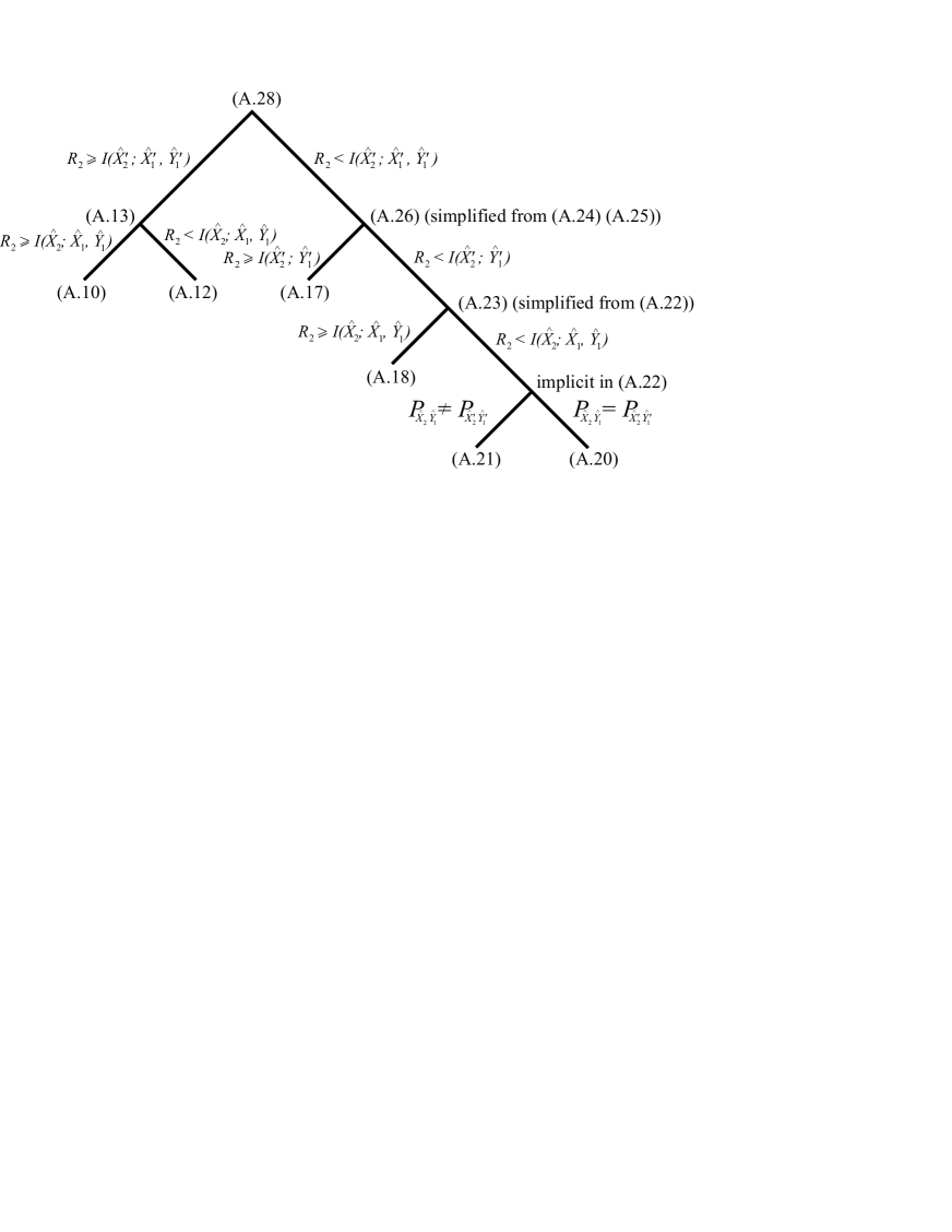
The bounding of requires considering multiple cases which depend on how compares to different information quantities, and also depend on properties of the joint types . In order to guide the reader through the different steps we present in Fig. 5 below a schematic representation of the different cases that arise.
We first consider two different ranges of ,
according to its comparison with :
1. The range . Here we have:
(A.7)
where in the second to last inequality we used ,
and in the last inequality we used the fact that
for any ,
which decays doubly exponentially with
(cf. [7, Appendix]).
To compute
we consider two cases, according to the
comparison between and :
The case . Here, we have:
(A.9)
Therefore, when
we have:
(A.10)
The case . Here we have:
(A.11)
where we used the fact that and then
estimated the expectation of as times
the probability would fall into the corresponding
conditional type.
Therefore, when
we have:
(A.12)
The exponents for the subcases and corresponding
to and , respectively, differ only
in the factors ( and , resp.) multiplying the term .
Therefore, we can consolidate these two subscases of into the expression:
(A.13)
since is when and when .
2. The range .
In this range,
where we assumed in the last step.
The second expectation over can be evaluated as
(A.15)
where
is the number of codewords that are jointly typical with
according to .
Thus,
(A.16)
To bound , we consider two
cases depending on how compares to .
The case . Here, we have:
(A.17)
where we used the fact that
decays doubly exponentially in the third inequality,
and bounded using (A.9) and (A.11)
in the last inequality.
The case . Here,
we further split the evaluation into two parts.
In the first part, , and we have:
(A.18)
where we used in the last inequality
valid for .
The other part corresponds to .
Here we have:
(A.19)
To bound , we consider two cases:
The first case is when :
in this case, . Therefore,
This completes the decomposition of into the various
subcases.
Figure 5: Tree representing the multiple ranges of considered in the derivation, and the equations that consolidate the different ranges.
Consolidation.
Next, we carry out a consolidation process that merges all of the above
subcases into a more compact expression, leading ultimately to the
expression in Theorem 1. Figure 5 gives a schematic representation, in terms of a tree, of the various consolidation steps described below. The consolidation of (A) and (A) into (A.13) was done before, but we include it in Fig. 5 for completeness. Referring to Fig. 5, the consolidation starts at the deepest leaves of the tree and works its way up the nodes until it reaches the root.
We begin with the last set of subsubcases derived,
and (expressions (A.18), (A.20), and
(A.21))
for the subcase , and consolidate them as follows:
(A.22)
Next we would like to decompose the indicator
appearing in the initial part of this expression as
where we are taking into account in the last step that for the present
subcase ,
since for
we have
.
Applying this decomposition to (A.22), then
combining terms having the same
indicators , and , and replacing indicators by as appropriate (similar to (A.13)),
we simplify (A.22) to
(A.23)
This is valid for the subcase
.
Next, we consolidate (A.17) from the subcase with (A.23) and insert the result
into (A.16) to get
(A.24)
which applies to the range .
Again, expanding all terms against the
indicators , and , and, as above, replacing indicators by as appropriate, we obtain
Similarly, we can decompose the term appearing after
the indicator
against the indicators and , and
use the above identity to combine it with
appearing after the indicator .
Incorporating these steps, we can rewrite (A.25) as
(A.26)
Finally, we consolidate (A.13) from the range
with the just obtained (A.26)
(for the range ) to get
(A.27)
As before, after expanding the first indicator
against , and , and combining terms, we obtain
(A.28)
where, in simplifying, we have made use of the identity
along with
and finally
We use (A.28) in (A),
add over all vectors , decompose all joint-type-dependent terms
appearing in (A), as well as the term
arising from the summation over per type, against the indicators
and ,
and finally optimize over the types ,
to obtain:
(A.29)
Note that the term mentioned above has been combined
with the term appearing in all subcases of (A.28) to
yield the appearing throughout (A.29).
The expression in Theorem 1 is obtained from (A.29)
by dropping the constraint from the first maximization (which, given
the continuity of the underlying terms, is not really a constraint
anyway), by noting that if, in the resulting expression, the second
maximization is attained
when , it will be dominated by the first maximization
so that the second maximization can be restricted to the case ,
and finally by negating the resulting exponent (and propagating the
negation as throughout).
Appendix B A Lower Bound to
We can lower bound the maximization of (3) over and
by applying the min-max
theorem twice, as follows.
First we introduce a new parameter
and bound (3) as
(B.1)
(B.2)
where and we have dropped the constraint involving from , resulting in a lower bound, and making convex.
Letting , we claim that for fixed ,
the expression in (B.2) being minimized over above is convex in . This follows from the fact that for fixed , both and are affine
in . The only problem would come from the ’s
appearing in these expressions, but it can be checked that these
maximizations are independent of for fixed . Letting , we can thus apply the min-max
theorem of convex analysis (twice) as follows
(B.3)
Since, as noted above, for fixed ( ), both and are
affine in , the inner maximization
in (B.3) is attained at one of the points . After simplification, we
obtain
Next, we note the identities
and use them, with the shorthand
and , for ,
to rewrite the bound as
(B.4)
where in simplifying the third expression in the maximization we have
also exploited the constraints
and .
For we can further simplify this expression. In
particular, for , the first term in the inner maximization
is readily seen to be always smaller than the second term.
Additionally, the second and third terms are symmetric in the primed
and non-primed joint distributions, which, together with the readily
established joint convexity
of the maximum of these two terms on the constraint set, imply that the inner
minimization over the joint types is achieved when the primed and
non-primed joint distributions are equal, in which case the two terms are equal.
Therefore, at
we have
(B.5)
or
(B.6)
where .
Simplifying at gives
(B.7)
which is seen to be no bigger than the above lower bound on , since
, , and .
Another application of the lower bound (B.4) is in
determining the set of rate pairs for which .
Let be independent with marginal distributions
and and be the result of
passing through the channel . We
shall argue that if .
and
then the expression (B.4) must be greater than 0.
Indeed, for the expression (B.4) to equal 0, we see from
the first term in the inner maximum that the
minimizing and joint distributions must satisfy one of the
following:
case 1: , , and ; case 2:
, , and ; or case 3:
, , and . If case 1 holds then
necessarily have the same joint distribution as , in which case, we see from the
third term in the maximum in (B.4) that . Similarly, if case 2 holds then it
follows that
have the same joint distribution as , in which case, it follows again
from the third term in the maximum that . Finally,
if case 3 holds then both and
have the same
distribution as , in which case, after writing , we see again that either or must hold. Thus, the three cases
together establish the above claim that if
and
then the expression (B.4), and hence ,
must be greater than 0. It can be checked that this region is
equivalent to
which is represented in Fig. 1 in Section IV.
It is shown in [11] that for
the ensemble of constant composition codes comprised of i.i.d. codewords
uniformly distributed over the types and ,
the exponential decay rate of the average probability of error for user 1
must necessarily be zero for rate pairs outside of this region, even
for optimum, maximum likelihood decoding.
References
[1] T. S. Han and K. Kobayashi, “A new achievable rate region for
the interference channel,” IEEE Trans. Info. Theory, vol. IT-27,
pp. 49 - 60, January 1981.
[2] A. B. Carleial, “A case where interference does not reduce capacity,”
(Corresp.), IEEE Trans. Info. Theory, vol. IT-21, pp. 569 -
570, September 1975.
[3] R. Etkin, D. Tse, and H. Wang, “Gaussian Interference Channel Capacity to Within One Bit,” submitted to IEEE Transactions on Information Theory, Feb. 2007. Also, available on–line at: [http://arxiv.org/PS_cache/cs/pdf/0702/0702045v2.pdf].
[4] L. Weng, S. S. Pradhan, and A. Anastasopoulos,
“Error exponent regions for Gaussian broadcast and multiple-access
channels,” IEEE Trans. Info. Theory, vol. IT-54, pp. 2919 - 2942,
July 2008.
[5] R. G. Gallager, Information Theory and Reliable Communication, John Wiley & Sons, Inc., New York, 1968.
[6] I. Csiszár, and J. Körner, Information Theory: Coding Theorems for Discrete Memoryless Systems, Akadémiai Kiadó, Budapest, 1981.
[7] N. Merhav, “Relations between random coding exponents and the statistical physics of random codes,” accepted to IEEE Trans. Inform. Theory, Sep. 2008. Also, available on–line at: [http://www.ee.technion.ac.il/people/merhav/papers/p117.pdf].
[8] N. Merhav, “Error exponents of erasure/list decoding
revisited via moments of distance enumerators,” IEEE Trans. Inform. Theory, Vol. 54, No. 10, pp. 4439-4447, Oct. 2008.
[9] R. Etkin, N. Merhav, E. Ordentlich, “Error exponents of optimum decoding for the interference channel,” Proceedings of the IEEE International Symposium on Information Theory, Toronto, Canada, pp. 1523–1527, 6-11 July 2008.
[10] R. Etkin, E. Ordentlich, “Discrete Memoryless Interference Channel: New Outer Bound,” Proceedings of the IEEE International Symposium on Information Theory, Nice, France, pp. 2851–2855, 24-29 June 2007.
[11] C. Chang, HP Labs Technical Report, 2008.
[12] J. Pokorny, H. Wallmeier, “Random coding bound and codes produced by permutations for the multiple-access channel,” IEEE Trans. Inform. Theory, Vol. 31, No. 6, pp. 741–750, Nov. 1985.
[13] Yu-Sun Liu, B. L. Hughes, “A new universal random coding bound for the multiple-access channel,” IEEE Trans. Inform. Theory, Vol. 42, No. 2, pp. 376–386, Mar. 1996.