Escaping Saddle Points in Distributed Newton’s Method with Communication Efficiency and Byzantine Resilience
Abstract
The problem of saddle-point avoidance for non-convex optimization is quite challenging in large scale distributed learning frameworks, such as Federated Learning, especially in the presence of Byzantine workers. The celebrated cubic-regularized Newton method of [Nesterov and Polyak(2006)] is one of the most elegant ways to avoid saddle-points in the standard centralized (non-distributed) setup. In this paper, we extend the cubic-regularized Newton method to a distributed framework and simultaneously address several practical challenges like communication bottleneck and Byzantine attacks. Note that the issue of saddle-point avoidance becomes more crucial in the presence of Byzantine machines since rogue machines may create fake local minima near the saddle-points of the loss function, also known as the saddle-point attack. Being a second order algorithm, our iteration complexity is much lower than the first order counterparts. Furthermore we use compression (or sparsification) techniques like -approximate compression for communication efficiency. We obtain theoretical guarantees for our proposed scheme under several settings including approximate (sub-sampled) gradients and Hessians. Moreover, we validate our theoretical findings with experiments using standard datasets and several types of Byzantine attacks, and obtain an improvement of with respect to first order methods in iteration complexity.
keywords:
Distributed optimization, Communication efficiency, robustness, compression.1 Introduction
Motivated by the real-world applications such as recommendation systems, image recognition, and conversational AI, it has become crucial to implement learning algorithms in a distributed fashion. In a commonly used framework, namely data-parallelism, large data-sets are distributed among several worker machines for parallel processing. In many applications, like Federated Learning (FL) [Konečnỳ et al.(2016)Konečnỳ, McMahan, Ramage, and Richtárik], data is stored in user devices such as mobile phones and personal computers. In a standard distributed framework, several worker machines perform local computations and communicate to the center machine (a parameter server), and the center machine aggregates and broadcasts the information iteratively.
In this setting, it is well-known that one of the major challenges is to tackle the behavior of the Byzantine machines [Lamport et al.(1982)Lamport, Shostak, and Pease]. This can happen owing to software or hardware crashes, poor communication link between the worker and the center machine, stalled computations, and even co-ordinated or malicious attacks by a third party. In this setup, it is generally assumed (see [Yin et al.(2018)Yin, Chen, Kannan, and Bartlett, Blanchard et al.(2017)Blanchard, Mhamdi, Guerraoui, and Stainer] that a subset of worker machines behave completely arbitrarily even in a way that depends on the algorithm used and the data on the other machines, thereby capturing the unpredictable nature of the errors.
Another critical challenge in this distributed setup is the communication cost between the worker and the center machine. The gains we obtain by parellelization of the task among several worker machines often get bottle-necked by the communication cost between the worker and the center machine. In applications like Federated learning, this communication cost is directly linked with the (internet) bandwidth of the users and thus resource constrained. It is well known that in-terms of the number of iterations, second order methods (like Newton and its variants) outperform their competitor; the first order gradient based methods. In this work, we simultaneously handle the Byzantine and communication cost aspects of distributed optimization for non-convex functions.
In this paper, we focus on optimizing a non-convex loss function in a distributed optimization framework. We have worker machines, out of which fraction may behave in a Byzantine fashion, where . Optimizing a loss function in a distributed setup has gained a lot of attention in recent years [Alistarh et al.(2018a)Alistarh, Allen-Zhu, and Li, Blanchard et al.(2017)Blanchard, Mhamdi, Guerraoui, and Stainer, Feng et al.(2014)Feng, Xu, and Mannor, Chen et al.(2017)Chen, Su, and Xu]. However, most of these approaches either work when is convex, or provide weak guarantees in the non-convex case (for example: zero gradient points, maybe a saddle point).
In order to fit complex machine learning models, one often requires to find local minima of a non-convex loss , instead of critical points only, which may include several saddle points. Training deep neural networks and other high-capacity learning architectures [Soudry and Carmon(2016), Ge et al.(2017)Ge, Jin, and Zheng] are some of the examples where finding local minima is crucial. [Ge et al.(2017)Ge, Jin, and Zheng, Kawaguchi(2016)] shows that the stationary points of these problems are in fact saddle points and far away from any local minimum, and hence designing efficient algorithm that escapes saddle points is of interest. Moreover, [Jain et al.(2017)Jain, Jin, Kakade, and Netrapalli, Sun et al.(2016)Sun, Qu, and Wright] argue that saddle points can lead to highly sub-optimal solutions in many problems of interest. This is amplified in high dimension as shown in [Dauphin et al.(2014)Dauphin, Pascanu, Gulcehre, Cho, Ganguli, and Bengio], and becomes the main bottleneck in training deep neural nets. Furthermore, a line of recent work [Sun et al.(2016)Sun, Qu, and Wright, Bhojanapalli et al.(2016)Bhojanapalli, Neyshabur, and Srebro, Sun et al.(2017)Sun, Qu, and Wright], shows that for many non-convex problems, it is sufficient to find a local minimum. In fact, in many problems of interest, all local minima are global minima (e.g., dictionary learning [Sun et al.(2017)Sun, Qu, and Wright], phase retrieval [Sun et al.(2016)Sun, Qu, and Wright], matrix sensing and completion [Bhojanapalli et al.(2016)Bhojanapalli, Neyshabur, and Srebro, Ge et al.(2017)Ge, Jin, and Zheng], and some of neural nets [Kawaguchi(2016)]). Also, in [Choromanska et al.(2015)Choromanska, Henaff, Mathieu, Arous, and LeCun], it is argued that for more general neural nets, the local minima are as good as global minima.
The issue of local minima convergence becomes non-trivial in the presence of Byzantine workers. Since we do not assume anything on the behavior of the Byzantine workers, it is certainly conceivable that by appropriately modifying their messages to the center, they can create fake local minima that are close to the saddle point of the loss function , and these are far away from the true local minima. This is popularly known as the saddle-point attack (see [Yin et al.(2019)Yin, Chen, Kannan, and Bartlett]), and it can arbitrarily destroy the performance of any non-robust learning algorithm. Hence, our goal is to design an algorithm that escapes saddle points of in an efficient manner as well as resists the saddle-point attack simultaneously. The complexity of such an algorithm emerges from the the interplay between non-convexity of the loss function and the behavior of the Byzantine machines.
The problem of saddle point avoidance in the context of non-convex optimization has received considerable attention in the past few years. In the seminal paper of [Jin et al.(2017)Jin, Ge, Netrapalli, Kakade, and Jordan], a (first order) gradient descent based approach is proposed. A few papers [Xu et al.(2017)Xu, Jin, and Yang, Allen-Zhu and Li(2017)] following the above use various modifications to obtain saddle point avoidance guarantees. A Byzantine robust first order saddle point avoidance algorithm is proposed by Yin et al. [Yin et al.(2019)Yin, Chen, Kannan, and Bartlett], and probably is the closest to this work. In [Yin et al.(2019)Yin, Chen, Kannan, and Bartlett], the authors propose a repeated check-and-escape type of first order gradient descent based algorithm. First of all, being a first order algorithm, the convergence rate is quite slow (the rate for gradient decay is , where is the number of iterations). Moreover, implementation-wise, the algorithm presented in [Yin et al.(2019)Yin, Chen, Kannan, and Bartlett] is computation heavy, and takes potentially many iterations between the center and the worker machines. Hence, this algorithm is not efficient in terms of the communication cost.
In this work, we consider a variation of the famous cubic-regularized Newton algorithm of Nesterov and Polyak [Nesterov and Polyak(2006)], which efficiently escapes the saddle points of a non-convex function by appropriately choosing a regularization and thus pushing the Hessian towards a positive semi-definite matrix. The primary motivation behind this choice is the faster convergence rate compared to first order methods, which is crucial in terms of communication efficiency in applications like Federated Learning. Indeed, the rate of gradient decay is .
We consider a distributed variant of the cubic regularized Newton algorithm. In this scheme, the center machine asks the workers to solve an auxiliary function and return the result. Note that the complexity of the problem is partially transferred to the worker machines. It is worth mentioning that in most distributed optimization paradigm, including Federated Learning, the workers posses sufficient compute power to handle this partial transfer of compute load, and in most cases, this is desirable [Konečnỳ et al.(2016)Konečnỳ, McMahan, Ramage, and Richtárik]. The center machine aggregates the solution of the worker machines and takes a descent step. Note that, unlike gradient aggregation, the aggregation of the solutions of the local optimization problems is a highly non-linear operation. Hence, it is quite non-trivial to extend the centralized cubic regularized algorithm to a distributed one. The solution to the cubic regularization even lacks a closed form solution unlike the second order Hessian based update or the first order gradient based update. The analysis is carried out by leveraging the first order and second order stationary conditions of the auxiliary function solved in each worker machines.
In addition to this, we simulateneously use (i) a -approximate compressor (defined shortly) to compress the message send from workers to center to gain further communication reduction and (ii) a simple norm-based thresholding to robustify against adversarial attacks. Norm based thresholding is a standard trick for Byzantine resilience as featured in [Ghosh et al.(2020a)Ghosh, Maity, Kadhe, Mazumdar, and Ramchandran, Ghosh et al.(2020b)Ghosh, Maity, and Mazumdar]. However, since the local optimization problem lacks a closed form solution, using norm-based trimming is also technical challenging in this case. We now list our contributions.
1.1 Our Contributions
We propose a novel distributed and robust cubic regularized Newton algorithm, that escapes saddle point efficiently. We prove that the algorithm convergence at a rate of , which is faster than the first order methods (which converge at rate, see [Yin et al.(2019)Yin, Chen, Kannan, and Bartlett]). Also, the rate matches to the centralized scheme of [Nesterov and Polyak(2006)] and hence, we do not lose in terms of convergence rate while making the algorithm distributed. We emphasis that since the center machine aggregates solutions of local (auxiliary) loss functions, this extension is quite non-trivial and technically challenging. This fast convergence reduces the number of iterations (and hence the communication cost) required to achieve a target accuracy.
Along with the saddle point avoidance, we simultaneously address the issues of (i) communication efficiency and (ii) Byzantine resilience by using a -approximate compressor and a norm-based thresholding scheme respectively. A major technical challenge here is to simultaneously address the above mentioned issues, and it turns out that with a proper parameter choice (step size etc.) it is possible to carry out the analysis jointly.
In Section 4, we verify our theoretical findings via experiments. We use benchmark LIBSVM ([Chang and Lin(2011)]) datasets for logistic regression and non-convex robust regression and show convergence results for both non-Byzantine and several different Byzantine attacks. Specifically, we characterize the total iteration complexity (defined in Section 4) of our algorithm, and compare it with the first order methods. We observe that the algorithm of [Yin et al.(2019)Yin, Chen, Kannan, and Bartlett] requires more total iterations than ours.
Preliminaries:
A point is said to satisfy the -second order stationary condition of if,
denotes the gradient of the function and denotes the minimum eigenvalue of the Hessian of the function. Hence, under the assumption (which is standard in the literature, see [Jin et al.(2017)Jin, Ge, Netrapalli, Kakade, and Jordan, Yin et al.(2019)Yin, Chen, Kannan, and Bartlett]) that all saddle points are strict (i.e., for any saddle point ), all second order stationary points (with ) are local minima, and hence converging to a stationary point is equivalent to converging to a local minima.
1.2 Problem Formulation
We minimize a loss function of the form: , where the function is twice differentiable and non-convex. In this work, we consider distributed optimization framework with worker machines and one center machine where the worker machines communicate to the center machine. Each worker machine is associated with a local loss function . We assume that the data distribution is non-iid across workers, which is standard in frameworks like FL. In addition to this, we also consider the case where fraction of the worker machines are Byzantine for some . The Byzantine machines can send arbitrary updates to the central machine which can disrupt the learning. Furthermore, the Byzantine machines can collude with each other, create fake local minima or attack maliciously by gaining information about the learning algorithm and other workers. In the rest of the paper, the norm will refer to norm or spectral norm when the argument is a vector or a matrix respectively.
Next, we consider a generic class of compressors from [Karimireddy et al.(2019)Karimireddy, Rebjock, Stich, and Jaggi]:
Definition 1.1 (-Approximate Compressor).
An operator is defined as approximate compressor on a set if, , , where is the compression factor.
Furthermore, a randomized operator is -approximate compressor on a set if, the above holds on expectation. In this paper, for the clarity of exposition, we consider the deterministic form of the compressor (as in Definition 1.1). However, the results can be easily extended for randomized . Notice that implies (no compression).
2 Related Work
Saddle Point avoidance algorithms:
In the recent years, there are handful first order algorithms [Lee et al.(2016)Lee, Simchowitz, Jordan, and Recht, Lee et al.(2017)Lee, Panageas, Piliouras, Simchowitz, Jordan, and Recht, Du et al.(2017)Du, Jin, Lee, Jordan, Poczos, and Singh] that focus on the escaping saddle points and convergence to local minima. The critical algorithmic aspect is running gradient based algorithm and adding perturbation to the iterates when the gradient is small. ByzantinePGD [Yin et al.(2019)Yin, Chen, Kannan, and Bartlett], PGD [Jin et al.(2017)Jin, Ge, Netrapalli, Kakade, and Jordan], Neon+GD[Xu et al.(2017)Xu, Jin, and Yang], Neon2+GD [Allen-Zhu and Li(2017)] are examples of such algorithms. The work of Nesterov and Polyak [Nesterov and Polyak(2006)] first proposes the cubic regularized second order Newton method and provides analysis for the second order stationary condition. An algorithm called Adaptive Regularization with Cubics (ARC) was developed by [Cartis et al.(2011a)Cartis, Gould, and Toint, Cartis et al.(2011b)Cartis, Gould, and Toint] where cubic regularized Newton method with access to inexact Hessian was studied. Cubic regularization with both the gradient and Hessian being inexact was studied in [Tripuraneni et al.(2018)Tripuraneni, Stern, Jin, Regier, and Jordan]. In [Kohler and Lucchi(2017)], a cubic regularized Newton with sub-sampled Hessian and gradient was proposed and analyzed. Momentum based cubic regularized algorithm was studied in [Wang et al.(2020)Wang, Zhou, Liang, and Lan]. A variance reduced cubic regularized algorithm was proposed in [Zhou et al.(2018)Zhou, Xu, and Gu, Wang et al.(2019)Wang, Zhou, Liang, and Lan]. In terms of solving the cubic sub-problem, [Carmon and Duchi(2016)] proposes a gradient based algorithm and [Agarwal et al.(2017)Agarwal, Allen-Zhu, Bullins, Hazan, and Ma] provides a Hessian-vector product technique.
Compression:
In the recent years, several gradient quantization or sparsification schemes have been studied in [Gandikota et al.(2019)Gandikota, Maity, and Mazumdar, Alistarh et al.(2017b)Alistarh, Grubic, Liu, Tomioka, and Vojnovic, Alistarh et al.(2018b)Alistarh, Hoefler, Johansson, Konstantinov, Khirirat, and Renggli, Wang et al.(2018)Wang, Sievert, Liu, Charles, Papailiopoulos, and Wright, Wen et al.(2017)Wen, Xu, Yan, Wu, Wang, Chen, and Li, Alistarh et al.(2017a)Alistarh, Grubic, Li, Tomioka, and Vojnovic, Ivkin et al.(2019)Ivkin, Rothchild, Ullah, Braverman, Stoica, and Arora]. In [Karimireddy et al.(2019)Karimireddy, Rebjock, Stich, and Jaggi], the authors introduced the idea of -approximate compressor. In [Ghosh et al.(2020c)Ghosh, Maity, Mazumdar, and Ramchandran], the authors used -approximate compressor to sparsify the second order update.
Byzantine resilience:
The effect of adversaries on convergence of non-convex optimization was studied in [Damaskinos et al.(2019)Damaskinos, El Mhamdi, Guerraoui, Guirguis, and Rouault, Mhamdi et al.(2018)Mhamdi, Guerraoui, and Rouault]. In the distributed learning context, [Feng et al.(2014)Feng, Xu, and Mannor] proposes one shot median based robust learning. A median of mean based algorithm was proposed in [Chen et al.(2017)Chen, Su, and Xu] where the worker machines are grouped in batches and the Byzantine resilience is achieved by computing the median of the grouped machines. Later [Yin et al.(2018)Yin, Chen, Kannan, and Bartlett] proposes co-ordinate wise median, trimmed mean and iterative filtering based approaches. Communication-efficient and Byzantine robust algorithms were developed in [Bernstein et al.(2018)Bernstein, Zhao, Azizzadenesheli, and Anandkumar, Ghosh et al.(2020a)Ghosh, Maity, Kadhe, Mazumdar, and Ramchandran]. A norm based thresholding approach for Byzantine resilience for distributed Newton algorithm was also developed [Ghosh et al.(2020b)Ghosh, Maity, and Mazumdar]. All these works provide only first order convergence guarantee (small gradient). The work [Yin et al.(2019)Yin, Chen, Kannan, and Bartlett] is the only one that provides second order guarantee (Hessian positive semi-definite) under Byzantine attack.
3 Compression, Byzantine Resilience and Distributed Cubic Regularized Newton
In this section, we describe a communication efficient and Byzantine robust distributed cubic Newton algorithm that can avoid saddle point by meeting the condition second order stationary point and thus converge to a local minima for non-convex loss function. Starting with initialization , the center machine broadcasts the parameter to the worker machines. At -th iteration, the -th worker machine solves a cubic-regularized auxiliary loss function based on its local data:
| (1) |
where are parameter choose suitably and are the gradient and Hessian of the local loss function computed on data stored in the worker machine.
After solving the problem described in (1), each worker machine applies compression operator as defined in Definition 1.1 on update . The application of the compression on the update is to minimize the communication cost.
Moreover, we also consider that fraction of the worker machines are Byzantine in nature. We denote the set of Byzantine worker machines by and the set of the rest of the good machines as . In each iteration, the good machines send the compressed update of solution of the sub-cubic problem described in equation (1) and the Byzantine machines can send any arbitrary values or intentionally disrupt the learning algorithm with malicious updates. Moreover, in the non-convex optimization problems, one of the more complicated and important issue is to avoid saddle points which can yield highly sub-optimal results. In the presence of Byzantine worker machines, they can be in cohort to create a fake local minima and drive the algorithm into sub-optimal region. Lack of any robust measure towards these type of intentional and unintentional attacks can be catastrophic to the learning procedure as the learning algorithm can get stuck in such sub-optimal point. To tackle such Byzantine worker machines, we employ a simple process called norm based thresholding.
After receiving all the updates from the worker machines, the central machine outputs a set which consists of the indexes of the worker machines with smallest norm. We choose the size of the set to be . Hence, we ‘trim’ fraction of the worker machine so that we can control the iterated update by not letting the worker machines with large norm participate and diverge the learning process. We denote the set of trimmed machine as . We choose so that at least one of the good machines gets trimmed. In this way, the norm of the all the updates in the set is bounded by at least the largest norm of the good machines.
Notice that the -approximate compressor is used to minimize the cost of communication and the norm based thresholding is used to mitigate the effect of the Byzantine machines. The central machine updates the parameter, with step-size as .
Remark 3.1.
Note that, we introduce the parameter in the cubic regularized sub-problem. The parameter emphasizes the effect of the second and third order terms in the sub-problem. The choice of plays an important role in our analysis in handling the non-linear update from different worker machines. Such non-linearity vanishes if we choose .
3.1 Theoretical Guarantees
We have the following standard assumptions:
Assumption 1
The non-convex loss function is twice continuously-differentiable and bounded below, i.e., .
Assumption 2
The loss is -Lipschitz continuous (, ), has -Lipschitz gradients and -Lipschitz Hessian
.
The above assumption states that the loss and the gradient and Hessian of the loss do not drastically change in the local neighborhood. These assumptions are standard in the analysis of the saddle point escape for cubic regularization (see [Tripuraneni et al.(2018)Tripuraneni, Stern, Jin, Regier, and Jordan, Kohler and Lucchi(2017), Nesterov and Polyak(2006), Carmon and Duchi(2016)]).
We assume the data distribution across workers to be non-iid. However, we assume that the local gradient and Hessian computed at worker machines (using local data) satisfies the following gradient and Hessian dissimilarity conditions. Note that these conditions are only applicable for non-Byzantine machines only. Byzantine machines do not adhere to any assumptions.
Assumption 3
(Gradient dissimilarity) For , we have for all .
Assumption 4
(Hessian dissimilarity) For , we have for all .
Similar assumptions featured in previous literature. For example, in [Karimireddy et al.(2020)Karimireddy, Kale, Mohri, Reddi, Stich, and Suresh, Fallah et al.(2020)Fallah, Mokhtari, and Ozdaglar], the authors use similar kind of dissimilarity assumptions that are prevalent in the Federated learning setup to highlight the non-iid or heterogeneity of the data among users.
Remark 3.2.
[Values of and in special cases] Compared to the Assumptions 3 and 4, the gradient and Hessian bound have been studied under more relaxed condition. In [Kohler and Lucchi(2017), Tripuraneni et al.(2018)Tripuraneni, Stern, Jin, Regier, and Jordan, Wang et al.(2020)Wang, Zhou, Liang, and Lan], the authors consider gradient and Hessian with sub-sampled data being drawn uniformly randomly from the data set. Due to the data being drawn in iid manner, both the bound parameters value diminish at the rate where is the size of the data sample in each worker machine. In [Ghosh et al.(2020b)Ghosh, Maity, and Mazumdar], the authors analyze the deviation in case of data partitioning where each worker node sample data uniformly without replacement from a given data set.
Theorem 3.3.
Remark 3.4.
Both the gradient and the minimum eigenvalue of the Hessian in the Theorem 3.3 have two parts. The first part decreases with the number iterations . The gradient and the minimum eigenvalue of the Hessian have the rate of and , respectively. Both of these rates match the rates of the centralized version of the cubic regularized Newton. In the second parts of the gradient bound and the minimum eigenvalue of the Hessian have terms with factor. As mentioned above (see Remark 3.2 ), in the special cases, both the terms and decrease at the rate of , where is the number of data in each of the worker machines.
Remark 3.5.
[Comparison with [Yin et al.(2019)Yin, Chen, Kannan, and Bartlett]] In a recent work, [Yin et al.(2019)Yin, Chen, Kannan, and Bartlett] provides a perturbed gradient based algorithm to escape the saddle point in non-convex optimization in the presence of Byzantine worker machines. Also, in that paper, the Byzantine resilience is achieved using techniques such as trimmed mean, median and collaborative filtering. These methods require additional assumptions (coordinate of the gradient being sub-exponential etc.) for the purpose of analysis. In this work, we do not require such assumptions. Moreover, we perform a simple norm based thresholding that provides robustness. Also the perturbed gradient descent (PGD) actually requires multiple rounds of communications between the central machine and the worker machines whenever the norm of the gradient is small as this is an indication of either a local minima or a saddle point. In contrast to that, our method does not require any additional communication for escaping the saddle points. Our method provides such ability by virtue of cubic regularization.
Remark 3.6.
Since our algorithm is second order in nature, it requires less number of iterations compared to the first order gradient based algorithms. Our algorithm achieves a superior rate of compared to the gradient based approach of rate . Our algorithm dominates ByzantinePGD [Yin et al.(2019)Yin, Chen, Kannan, and Bartlett] in terms of convergence, communication rounds and simplicity.
We now state two corollaries. First, we relax the condition of compression by choosing . The worker machines communicate the actual update instead of the compressed the update.
Corollary 3.7 (No compression).
Next, we choose the non-Byzantine setup with in addition to the uncompressed update. This is just the distributed variant of the cubic regularized Newton method.
Corollary 3.8 (Non Byzantine and no compression).
Remark 3.9 (Two rounds of communication ).
We can improve the bound in the Corollary 3.8, with the calculation of the actual gradient which requires one more round of communication in each iteration. In the first iteration, all the worker machines compute the gradient based on the stored data and send it to the center machine. The center machine averages them and then broadcast the global gradient at iteration . In this manner, the worker machines solve the sub-problem (1) with the actual gradient. This improves the gradient bound while the communication remains in each iteration.
3.2 Solution of the cubic sub-problem
The cubic regularized sub-problem (1) needs to be solved to update the parameter. As this particular problem does not have a closed form solution, a solver is usually employed which yields a satisfactory solution. In previous works, different types of solvers have been used. [Cartis et al.(2011a)Cartis, Gould, and Toint, Cartis et al.(2011b)Cartis, Gould, and Toint] solve the sub-problem using Lanczos based method in Krylov subspace. In [Agarwal et al.(2017)Agarwal, Allen-Zhu, Bullins, Hazan, and Ma], the authors propose a solver based on Hessian-vector product and binary search. Gradient descent based solver is proposed in [Carmon and Duchi(2016), Tripuraneni et al.(2018)Tripuraneni, Stern, Jin, Regier, and Jordan].
Previous works, [Wang et al.(2020)Wang, Zhou, Liang, and Lan, Zhou et al.(2018)Zhou, Xu, and Gu, Wang et al.(2019)Wang, Zhou, Liang, and Lan], consider the exact solution of the cubic sub-problem for theoretical analysis. Recently, inexact solutions to the sub-problem is also proposed in the centralized (non-distributed) framework. For instance, [Kohler and Lucchi(2017)] analyzes the cubic model with sub-sampled Hessian with approximate model minimization technique developed in [Cartis et al.(2011a)Cartis, Gould, and Toint]. Moreover, [Tripuraneni et al.(2018)Tripuraneni, Stern, Jin, Regier, and Jordan] shows improved analysis with gradient based minimization which is a variant studied in [Carmon and Duchi(2016)]. Both exact and inexact solutions to the sub-problem yields similar theoretical guarantees.
In our framework, each worker machine is tasked with solving the sub-problem. For the purpose of theoretical convergence analysis, we consider that woker machines obtain the exact solution in each round. However, in experiments (Section 4), we apply the gradient based solver of [Tripuraneni et al.(2018)Tripuraneni, Stern, Jin, Regier, and Jordan] to solve the sub-problem. Here, we let each worker machines run the gradient based solver for iterations and send the update to the center machine in each iteration.
4 Experimental Results
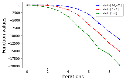
First we show that our algorithm indeed escapes saddle point with a toy example. We choose a dimensional example: where and (Here denotes the -th coordinate of . This problem is the sum of two non-convex function and has a saddle point at . In Figure 1 (left most) we observe that our algorithm escapes the saddle point , with random initialization.
Next, we validate our algorithm on benchmark LIBSVM ([Chang and Lin(2011)]) data-set in both convex and non-convex problems. We choose the following loss functions: (a) Logistic loss:, and (b) Non-convex robust linear regression: , where is the parameter, are the feature vectors and are the corresponding labels. We choose ‘a9a’(, we split the data into and use as training/testing purpose) and ‘w8a’(training data and testing data ) classification datasets and partition the data in 20 different worker machines.
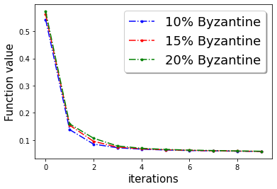
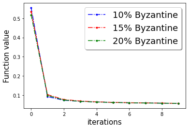
First, we demonstrate Algorithm 1 in the presence of Byzantine machines and compressed update. For compression, each worker applies compression operator of QSGD [Alistarh et al.(2017a)Alistarh, Grubic, Li, Tomioka, and Vojnovic]. For a given vector for all . In this work, we consider the following four Byzantine attacks: (1) ‘Gaussian Noise attack’: where the Byzantine worker machines add Gaussian noise to the update. (2) ‘Random label attack’: where the Byzantine worker machines train and learn based on random labels instead of the proper labels. (3) ‘Flipped label attack’: where (for Binary classification) the Byzantine worker machines flip the labels of the data and learn based on wrong labels. (4) ‘Negative update attack’: where the Byzantine workers computes the update (here solves the sub-problem in Eq. (1)) and communicates with making the direction of the update opposite of the actual one. In Figure 2, we plot the function value of the robust linear regression problem for ’flipped labels‘ and ’negative update‘ attacks with compressed update for both ‘w8a’ and ‘a9a’ dataset. We choose the parameters , learning rate , and , where number of worker machines . The results with Gaussian and random labels attacks are shown in Appendix.
[] \subfigure[]
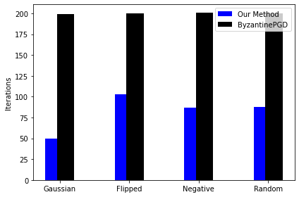 \subfigure[]
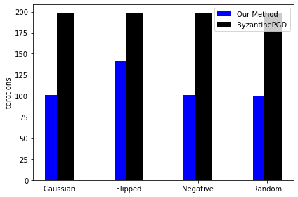 \subfigure[]
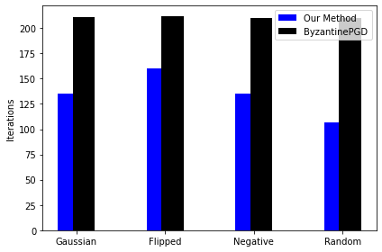
[] \subfigure[]
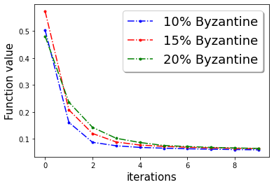 \subfigure[]
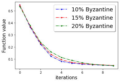 \subfigure[]
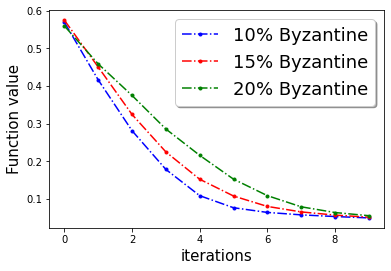
Comparison with [Yin et al.(2019)Yin, Chen, Kannan, and Bartlett]
: We compare our uncompressed version of the algorithm with ByzantinePGD of [Yin et al.(2019)Yin, Chen, Kannan, and Bartlett]. We take the total number of iterations as a comparison metric. One outer iteration of Algorithm 1 corresponds to one round of communication between the center and the worker machines (and hence one parameter update). Note that in our algorithm the worker machines use 10 steps of gradient solver (see [Tripuraneni et al.(2018)Tripuraneni, Stern, Jin, Regier, and Jordan]) for the local sub problem per iteration. So, the total number of iterations is given by times the number of outer iterations.For both the algorithms, we choose norm of the gradient as a stopping criteria. For ByzantinePGD, we choose and ‘co-ordinate wise Trimmed mean. In the Figure 1, we plot the total number of iterations in all four types of attacks with different fraction of Byzantine machines. It is evident from the plot that our method requires less number of over all iterations (at least , and less for , and of Byzantine machines respectively). We provide the results for the non-Byzantine case in the Appendix.
References
- [Agarwal et al.(2017)Agarwal, Allen-Zhu, Bullins, Hazan, and Ma] Naman Agarwal, Zeyuan Allen-Zhu, Brian Bullins, Elad Hazan, and Tengyu Ma. Finding approximate local minima faster than gradient descent. In Proceedings of the 49th Annual ACM SIGACT Symposium on Theory of Computing, pages 1195–1199, 2017.
- [Alistarh et al.(2017a)Alistarh, Grubic, Li, Tomioka, and Vojnovic] Dan Alistarh, Demjan Grubic, Jerry Li, Ryota Tomioka, and Milan Vojnovic. Qsgd: Communication-efficient sgd via gradient quantization and encoding. In Advances in Neural Information Processing Systems, pages 1709–1720, 2017a.
- [Alistarh et al.(2017b)Alistarh, Grubic, Liu, Tomioka, and Vojnovic] Dan Alistarh, Demjan Grubic, Jerry Liu, Ryota Tomioka, and Milan Vojnovic. Communication-efficient stochastic gradient descent, with applications to neural networks. 2017b.
- [Alistarh et al.(2018a)Alistarh, Allen-Zhu, and Li] Dan Alistarh, Zeyuan Allen-Zhu, and Jerry Li. Byzantine stochastic gradient descent. In Advances in Neural Information Processing Systems, volume 31, pages 4613–4623, 2018a.
- [Alistarh et al.(2018b)Alistarh, Hoefler, Johansson, Konstantinov, Khirirat, and Renggli] Dan Alistarh, Torsten Hoefler, Mikael Johansson, Nikola Konstantinov, Sarit Khirirat, and Cédric Renggli. The convergence of sparsified gradient methods. In Advances in Neural Information Processing Systems, pages 5973–5983, 2018b.
- [Allen-Zhu and Li(2017)] Zeyuan Allen-Zhu and Yuanzhi Li. Neon2: Finding local minima via first-order oracles. arXiv preprint arXiv:1711.06673, 2017.
- [Bernstein et al.(2018)Bernstein, Zhao, Azizzadenesheli, and Anandkumar] Jeremy Bernstein, Jiawei Zhao, Kamyar Azizzadenesheli, and Anima Anandkumar. signsgd with majority vote is communication efficient and byzantine fault tolerant. arXiv preprint arXiv:1810.05291, 2018.
- [Bhojanapalli et al.(2016)Bhojanapalli, Neyshabur, and Srebro] Srinadh Bhojanapalli, Behnam Neyshabur, and Nathan Srebro. Global optimality of local search for low rank matrix recovery, 2016.
- [Blanchard et al.(2017)Blanchard, Mhamdi, Guerraoui, and Stainer] Peva Blanchard, El Mahdi El Mhamdi, Rachid Guerraoui, and Julien Stainer. Byzantine-tolerant machine learning. arXiv preprint arXiv:1703.02757, 2017.
- [Carmon and Duchi(2016)] Yair Carmon and John C Duchi. Gradient descent efficiently finds the cubic-regularized non-convex newton step. arXiv preprint arXiv:1612.00547, 2016.
- [Cartis et al.(2011a)Cartis, Gould, and Toint] Coralia Cartis, Nicholas IM Gould, and Philippe L Toint. Adaptive cubic regularisation methods for unconstrained optimization. part i: motivation, convergence and numerical results. Mathematical Programming, 127(2):245–295, 2011a.
- [Cartis et al.(2011b)Cartis, Gould, and Toint] Coralia Cartis, Nicholas IM Gould, and Philippe L Toint. Adaptive cubic regularisation methods for unconstrained optimization. part ii: worst-case function-and derivative-evaluation complexity. Mathematical programming, 130(2):295–319, 2011b.
- [Chang and Lin(2011)] Chih-Chung Chang and Chih-Jen Lin. Libsvm: A library for support vector machines. ACM transactions on intelligent systems and technology (TIST), 2(3):27, 2011.
- [Chen et al.(2017)Chen, Su, and Xu] Yudong Chen, Lili Su, and Jiaming Xu. Distributed statistical machine learning in adversarial settings: Byzantine gradient descent. Proceedings of the ACM on Measurement and Analysis of Computing Systems, 1(2):44, 2017.
- [Choromanska et al.(2015)Choromanska, Henaff, Mathieu, Arous, and LeCun] Anna Choromanska, Mikael Henaff, Michael Mathieu, Gérard Ben Arous, and Yann LeCun. The loss surfaces of multilayer networks, 2015.
- [Damaskinos et al.(2019)Damaskinos, El Mhamdi, Guerraoui, Guirguis, and Rouault] Georgios Damaskinos, El Mahdi El Mhamdi, Rachid Guerraoui, Arsany Hany Abdelmessih Guirguis, and Sébastien Louis Alexandre Rouault. Aggregathor: Byzantine machine learning via robust gradient aggregation. page 19, 2019. URL http://infoscience.epfl.ch/record/265684. Published in the Conference on Systems and Machine Learning (SysML) 2019, Stanford, CA, USA.
- [Dauphin et al.(2014)Dauphin, Pascanu, Gulcehre, Cho, Ganguli, and Bengio] Yann N Dauphin, Razvan Pascanu, Caglar Gulcehre, Kyunghyun Cho, Surya Ganguli, and Yoshua Bengio. Identifying and attacking the saddle point problem in high-dimensional non-convex optimization. In Advances in Neural Information Processing Systems, volume 27, pages 2933–2941, 2014.
- [Du et al.(2017)Du, Jin, Lee, Jordan, Poczos, and Singh] Simon S Du, Chi Jin, Jason D Lee, Michael I Jordan, Barnabas Poczos, and Aarti Singh. Gradient descent can take exponential time to escape saddle points. arXiv preprint arXiv:1705.10412, 2017.
- [Fallah et al.(2020)Fallah, Mokhtari, and Ozdaglar] Alireza Fallah, Aryan Mokhtari, and Asuman Ozdaglar. Personalized federated learning: A meta-learning approach. arXiv preprint arXiv:2002.07948, 2020.
- [Feng et al.(2014)Feng, Xu, and Mannor] Jiashi Feng, Huan Xu, and Shie Mannor. Distributed robust learning. arXiv preprint arXiv:1409.5937, 2014.
- [Gandikota et al.(2019)Gandikota, Maity, and Mazumdar] Venkata Gandikota, Raj Kumar Maity, and Arya Mazumdar. vqsgd: Vector quantized stochastic gradient descent. arXiv preprint arXiv:1911.07971, 2019.
- [Ge et al.(2017)Ge, Jin, and Zheng] Rong Ge, Chi Jin, and Yi Zheng. No spurious local minima in nonconvex low rank problems: A unified geometric analysis. In Proceedings of the 34th International Conference on Machine Learning, volume 70 of Proceedings of Machine Learning Research, pages 1233–1242, International Convention Centre, Sydney, Australia, 06–11 Aug 2017. PMLR.
- [Ghosh et al.(2020a)Ghosh, Maity, Kadhe, Mazumdar, and Ramchandran] Avishek Ghosh, Raj Kumar Maity, Swanand Kadhe, Arya Mazumdar, and Kannan Ramchandran. Communication-efficient and byzantine-robust distributed learning. In 2020 Information Theory and Applications Workshop (ITA), pages 1–28. IEEE, 2020a.
- [Ghosh et al.(2020b)Ghosh, Maity, and Mazumdar] Avishek Ghosh, Raj Kumar Maity, and Arya Mazumdar. Distributed newton can communicate less and resist byzantine workers. In Advances in Neural Information Processing Systems 33: Annual Conference on Neural Information Processing Systems 2020, NeurIPS 2020, December 6-12, 2020, virtual, 2020b.
- [Ghosh et al.(2020c)Ghosh, Maity, Mazumdar, and Ramchandran] Avishek Ghosh, Raj Kumar Maity, Arya Mazumdar, and Kannan Ramchandran. Communication efficient distributed approximate newton method. In 2020 IEEE International Symposium on Information Theory (ISIT), pages 2539–2544. IEEE, 2020c.
- [Ivkin et al.(2019)Ivkin, Rothchild, Ullah, Braverman, Stoica, and Arora] Nikita Ivkin, Daniel Rothchild, Enayat Ullah, Vladimir Braverman, Ion Stoica, and Raman Arora. Communication-efficient distributed sgd with sketching. arXiv preprint arXiv:1903.04488, 2019.
- [Jain et al.(2017)Jain, Jin, Kakade, and Netrapalli] Prateek Jain, Chi Jin, Sham M. Kakade, and Praneeth Netrapalli. Global convergence of non-convex gradient descent for computing matrix squareroot, 2017.
- [Jin et al.(2017)Jin, Ge, Netrapalli, Kakade, and Jordan] Chi Jin, Rong Ge, Praneeth Netrapalli, Sham M Kakade, and Michael I Jordan. How to escape saddle points efficiently. In International Conference on Machine Learning, pages 1724–1732. PMLR, 2017.
- [Karimireddy et al.(2019)Karimireddy, Rebjock, Stich, and Jaggi] Sai Praneeth Karimireddy, Quentin Rebjock, Sebastian Stich, and Martin Jaggi. Error feedback fixes signsgd and other gradient compression schemes. In International Conference on Machine Learning, pages 3252–3261. PMLR, 2019.
- [Karimireddy et al.(2020)Karimireddy, Kale, Mohri, Reddi, Stich, and Suresh] Sai Praneeth Karimireddy, Satyen Kale, Mehryar Mohri, Sashank Reddi, Sebastian Stich, and Ananda Theertha Suresh. Scaffold: Stochastic controlled averaging for federated learning. In International Conference on Machine Learning, pages 5132–5143. PMLR, 2020.
- [Kawaguchi(2016)] Kenji Kawaguchi. Deep learning without poor local minima. In D. Lee, M. Sugiyama, U. Luxburg, I. Guyon, and R. Garnett, editors, Advances in Neural Information Processing Systems, volume 29, pages 586–594. Curran Associates, Inc., 2016. URL https://proceedings.neurips.cc/paper/2016/file/f2fc990265c712c49d51a18a32b39f0c-Paper.pdf.
- [Kohler and Lucchi(2017)] Jonas Moritz Kohler and Aurelien Lucchi. Sub-sampled cubic regularization for non-convex optimization. In International Conference on Machine Learning, pages 1895–1904. PMLR, 2017.
- [Konečnỳ et al.(2016)Konečnỳ, McMahan, Ramage, and Richtárik] Jakub Konečnỳ, H Brendan McMahan, Daniel Ramage, and Peter Richtárik. Federated optimization: Distributed machine learning for on-device intelligence. arXiv preprint arXiv:1610.02527, 2016.
- [Lamport et al.(1982)Lamport, Shostak, and Pease] Leslie Lamport, Robert Shostak, and Marshall Pease. The byzantine generals problem. ACM Trans. Program. Lang. Syst., 4(3):382–401, July 1982. ISSN 0164-0925. 10.1145/357172.357176. URL http://doi.acm.org/10.1145/357172.357176.
- [Lee et al.(2016)Lee, Simchowitz, Jordan, and Recht] Jason D Lee, Max Simchowitz, Michael I Jordan, and Benjamin Recht. Gradient descent converges to minimizers. arXiv preprint arXiv:1602.04915, 2016.
- [Lee et al.(2017)Lee, Panageas, Piliouras, Simchowitz, Jordan, and Recht] Jason D Lee, Ioannis Panageas, Georgios Piliouras, Max Simchowitz, Michael I Jordan, and Benjamin Recht. First-order methods almost always avoid saddle points. arXiv preprint arXiv:1710.07406, 2017.
- [Mhamdi et al.(2018)Mhamdi, Guerraoui, and Rouault] El Mahdi El Mhamdi, Rachid Guerraoui, and Sébastien Rouault. The hidden vulnerability of distributed learning in byzantium. arXiv preprint arXiv:1802.07927, 2018.
- [Nesterov and Polyak(2006)] Yurii Nesterov and Boris T Polyak. Cubic regularization of newton method and its global performance. Mathematical Programming, 108(1):177–205, 2006.
- [Soudry and Carmon(2016)] Daniel Soudry and Yair Carmon. No bad local minima: Data independent training error guarantees for multilayer neural networks, 2016.
- [Sun et al.(2016)Sun, Qu, and Wright] Ju Sun, Qing Qu, and John Wright. A geometric analysis of phase retrieval. CoRR, abs/1602.06664, 2016. URL http://arxiv.org/abs/1602.06664.
- [Sun et al.(2017)Sun, Qu, and Wright] Ju Sun, Qing Qu, and John Wright. Complete dictionary recovery over the sphere i: Overview and the geometric picture. IEEE Transactions on Information Theory, 63(2):853–884, Feb 2017. ISSN 1557-9654. 10.1109/tit.2016.2632162. URL http://dx.doi.org/10.1109/TIT.2016.2632162.
- [Tripuraneni et al.(2018)Tripuraneni, Stern, Jin, Regier, and Jordan] N Tripuraneni, M Stern, C Jin, J Regier, and MI Jordan. Stochastic cubic regularization for fast nonconvex optimization. In Advances in Neural Information Processing Systems, pages 2899–2908, 2018.
- [Wang et al.(2018)Wang, Sievert, Liu, Charles, Papailiopoulos, and Wright] Hongyi Wang, Scott Sievert, Shengchao Liu, Zachary Charles, Dimitris Papailiopoulos, and Stephen Wright. Atomo: Communication-efficient learning via atomic sparsification. In Advances in Neural Information Processing Systems, pages 9850–9861, 2018.
- [Wang et al.(2019)Wang, Zhou, Liang, and Lan] Zhe Wang, Yi Zhou, Yingbin Liang, and Guanghui Lan. Stochastic variance-reduced cubic regularization for nonconvex optimization. In The 22nd International Conference on Artificial Intelligence and Statistics, pages 2731–2740. PMLR, 2019.
- [Wang et al.(2020)Wang, Zhou, Liang, and Lan] Zhe Wang, Yi Zhou, Yingbin Liang, and Guanghui Lan. Cubic regularization with momentum for nonconvex optimization. In Uncertainty in Artificial Intelligence, pages 313–322. PMLR, 2020.
- [Wen et al.(2017)Wen, Xu, Yan, Wu, Wang, Chen, and Li] Wei Wen, Cong Xu, Feng Yan, Chunpeng Wu, Yandan Wang, Yiran Chen, and Hai Li. Terngrad: Ternary gradients to reduce communication in distributed deep learning. In Advances in neural information processing systems, pages 1509–1519, 2017.
- [Xu et al.(2017)Xu, Jin, and Yang] Yi Xu, Rong Jin, and Tianbao Yang. First-order stochastic algorithms for escaping from saddle points in almost linear time. arXiv preprint arXiv:1711.01944, 2017.
- [Yin et al.(2018)Yin, Chen, Kannan, and Bartlett] Dong Yin, Yudong Chen, Ramchandran Kannan, and Peter Bartlett. Byzantine-robust distributed learning: Towards optimal statistical rates. In Proceedings of the 35th International Conference on Machine Learning, volume 80 of Proceedings of Machine Learning Research, pages 5650–5659, Stockholm, Sweden, 10–15 Jul 2018. PMLR.
- [Yin et al.(2019)Yin, Chen, Kannan, and Bartlett] Dong Yin, Yudong Chen, Ramchandran Kannan, and Peter Bartlett. Defending against saddle point attack in byzantine-robust distributed learning. In International Conference on Machine Learning, pages 7074–7084. PMLR, 2019.
- [Zhou et al.(2018)Zhou, Xu, and Gu] Dongruo Zhou, Pan Xu, and Quanquan Gu. Stochastic variance-reduced cubic regularized newton methods. In International Conference on Machine Learning, pages 5990–5999. PMLR, 2018.
5 Appendix
In this part, we establish some useful facts and lemmas. Next, we provide analysis of Theorems 3.3.
5.1 Some useful facts
For the purpose of analysis we use the following sets of inequalities.
Fact 1.
For we have the following inequality
| (5) | ||||
| (6) |
Fact 2.
For and
| (7) |
Lemma 5.1 ([Nesterov and Polyak(2006)]).
Under Assumption 2, i.e., the Hessian of the function is -Lipschitz continuous, for any , we have
| (8) | |||
| (9) |
Next, we establish the following Lemma that provides some nice properties of the cubic sub-problem.
Lemma 5.2.
Let , and
| (10) |
The following holds
| (11) | ||||
| (12) | ||||
| (13) |
5.2 Proof of Theorem 3.3
First we state the results of Lemma 5.2 for each worker machine in iteration ,
| (16) | ||||
| (17) | ||||
| (18) |
We also use the following fact form the setup and trimming set
| (19) | ||||
| (20) |
Combining both the equations (19) and (20), we have
| (21) |
Now we state the following fact from the trimming set
| Combining both we get | ||||
| (22) | ||||
For the rest of the calculation, we use the following notation
If the optimization sub-problem domain is bounded, can be upper-bounded by the diameter of the parameter space. Note that in the definition of , the maximum is taken over good machines only.
From the definition of the -approximate compressor in Definition 1.1, we use the following simple fact
| (23) |
At any iteration , we have
| (24) |
In the above calculation we use the fact gradients are bounded and the bound of gradient dissimilarity.
We use the result (22), we get
| (25) |
Now we use the fact in equation (22) and the definition of the -approximate compressor, we get
| (26) |
Now we consider the Term 2 in (24)
| (27) |
| (30) |
Now we combine all the upper bound of the Term 1, Term 2 and Term 3
Also we assume that and use the fact .
Now we have,
where
and
To ensure , we need
| (31) |
Now for the choice of and for some constant . We have . Thus we have and .
Now we have
Now we consider the step , where .
With the choice of we have the terms and are upper bounded by constant.
We have
where
And
where
So, we have both the term are of the order .
The gradient condition is
| (32) |
Now consider the term in (32)
Next we consider the term
| (33) |
So finally we have
Now we choose .
At step ,
where and as , we have .
The Hessian bound is
| (34) |
At we have
| (35) | ||||
| (36) |
where and we have .
We have the following parameters
| (37) |
6 Additional Experiments
In this section we provide additional experiments. We choose the parameters , learning rate , fraction of the Byzantine machines and .
Compressed and Byzantine:
In Figure 3, we plot the function value of the robust linear regression problem for ’Gaussian attack‘ and ’random label‘ attacks with compressed update for both ‘w8a’ and ‘a9a’ dataset.
[] \subfigure[]
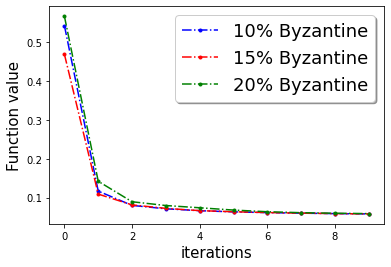 \subfigure[]
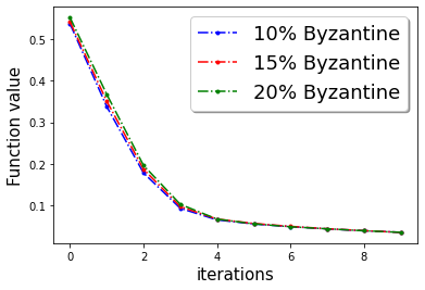 \subfigure[]
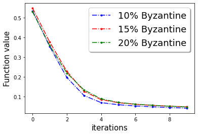
[] \subfigure[]
 \subfigure[]
 \subfigure[]
\subfigure[] \subfigure[]
 \subfigure[]
 \subfigure[]
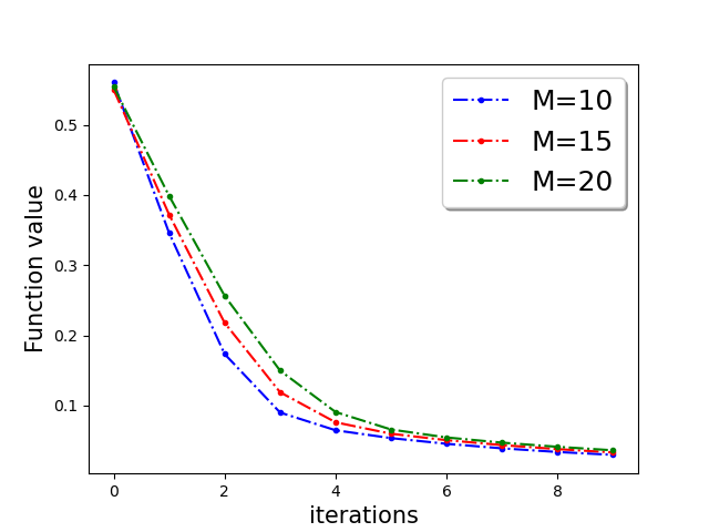
[] \subfigure[]
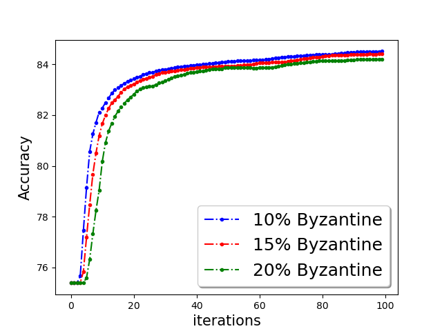 \subfigure[]
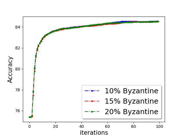 \subfigure[]
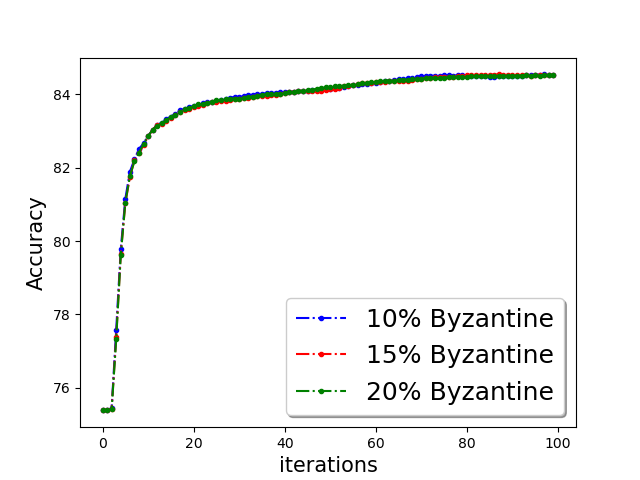
\subfigure[]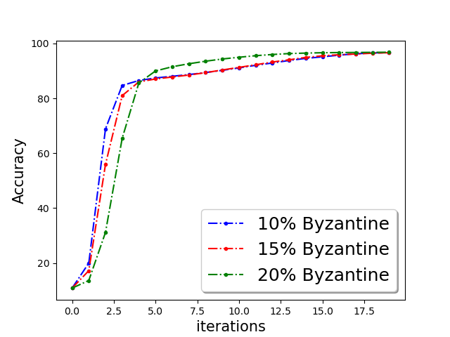 \subfigure[]
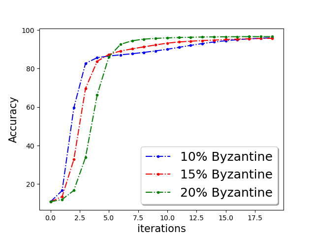 \subfigure[]
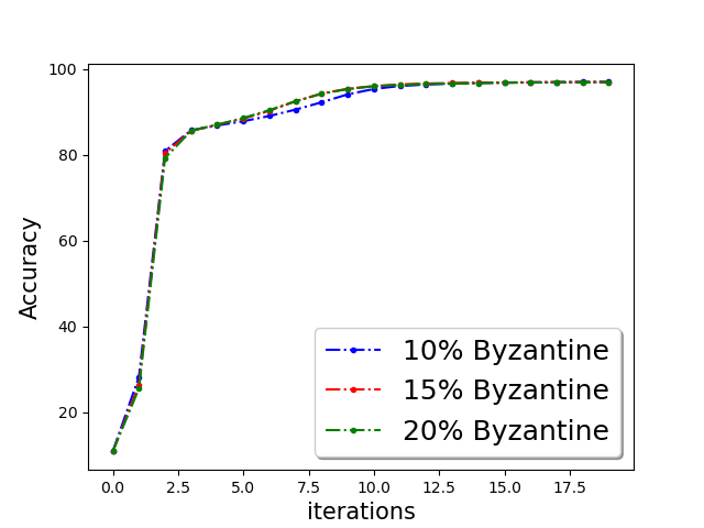 \subfigure[]
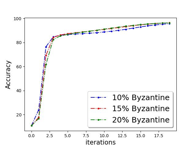
Training loss for uncompressed update:
In Figure 4, we plot the function value of the robust linear regression problem for all four attacks update for both ‘w8a’ and ‘a9a’ dataset with uncompressed update .
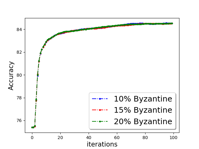
Classification accuracy:
We show the classification accuracy on testing data of ‘a9a’ and ‘w8a’ dataset for logistic regression problem in Figure 5 and training function loss of ‘a9a’ and ‘w8a’ dataset for robust linear regression problem in the Figure 5. It is evident from the plots that a simple norm based thresholding makes the learning algorithm robust.