Estimation of conditional average treatment effects on distributed confidential data
Abstract
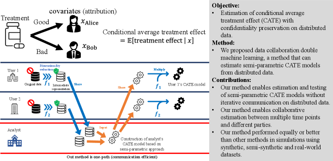
Estimation of conditional average treatment effects (CATEs) is an important topic in sciences. CATEs can be estimated with high accuracy if distributed data across multiple parties can be centralized. However, it is difficult to aggregate such data owing to confidential or privacy concerns. To address this issue, we proposed data collaboration double machine learning, a method that can estimate CATE models from privacy-preserving fusion data constructed from distributed data, and evaluated our method through simulations. Our contributions are summarized in the following three points. First, our method enables estimation and testing of semi-parametric CATE models without iterative communication on distributed data. Our semi-parametric CATE method enable estimation and testing that is more robust to model mis-specification than parametric methods. Second, our method enables collaborative estimation between multiple time points and different parties through the accumulation of a knowledge base. Third, our method performed equally or better than other methods in simulations using synthetic, semi-synthetic and real-world datasets.
Keywords— Statistical causal inference; Conditional average treatment effect; Privacy-preserving; Distributed data; Double machine learning
1 Introduction
The Neyman–Rubin model (Imbens and Rubin, 2015) or potential outcomes framework is one of the main causal inference methods for estimating average treatment (intervention) effects and has been developed and applied in many studies since its establishment by Rubin. In recent years, there have been innovations that enable the estimation of individual or conditional average treatment effects (CATEs) by adapting not only statistical but also machine learning methods (e.g., Künzel et al. (2019); Athey et al. (2019)). Most methods for estimating CATEs assume that the data can be centralized in one place. However, if the distributed data contains confidential or private information, it is difficult to centralized them in one place.
Conversely, in the field of machine learning, a privacy-preserving analysis method called federated learning has been developed in recent years (Konečnỳ et al., 2016; McMahan et al., 2017; Rodríguez-Barroso et al., 2020; Criado et al., 2022; Rodríguez-Barroso et al., 2023; Rafi et al., 2024). Data collaboration (DC) analysis (Imakura and Sakurai, 2020; Bogdanova et al., 2020; Imakura et al., 2021b, 2023b, 2023a), one of federated learning systems, is a method that enables collaborative analysis from privacy-preserving fusion data. The privacy-preserving fusion data are constructed by sharing dimensionality-reduced intermediate representations instead of raw data. DC analysis was originally proposed to address regression and classification problems in distributed data. Recently, Kawamata et al. (Kawamata et al., 2024) proposed data collaboration quasi-experiment (DC-QE), that extends DC analysis to allow estimation of average treatment effect (ATE). It is important to note that although those studies often focus their discussions on privacy data (personal information), the technologies can also be used to preserve the management information held by companies. Therefore, in this paper, we collectively refer to such data that are difficult to disclose to the outside as confidential information. Below we discuss techniques for preserving confidential information.
In this paper, we propose data collaboration double machine learning (DC-DML) as a method to estimate CATEs while preserving the confidentiality of distributed data by incorporating double machine learning (DML) (Chernozhukov et al., 2018), a machine learning-based treatment effect estimation method, into DC-QE. Moreover, through numerical simulations, we evaluate the performance of our method compared to existing methods.
This paper relates partially linear models, one of the semi-parametric models. Since Engle et al. (Engle et al., 1986), partially linear models have been used in empirical studies where assuming a linear model between the covariates and the outcome is not appropriate, i.e., to avoid model mis-specification owing to linear assumptions. A significant advance about partially linear models in recent years is DML (Chernozhukov et al., 2018), which brought an least square estimator that can adapt common machine learning models. Various causal inference methods have been developed by developing DML (Fan et al., 2022; Bia et al., 2023). In this paper, we develop DML into a method that enables CATE estimation through distributed data with privacy-preserving.
The effects of policy interventions by governments or medical treatments by hospitals are likely to differ across people. It is possible to improve the overall performance of the treatment if one knows which subjects should be treated. For example, by concentrating scholarship support on those whose future income increases will be higher owing to the treatment, the limited budget can be used more efficiently. In addition, by concentrating medication on those who are more likely to improved or have fewer side effects from the treatment, medication can be more effective and safer to use. One approach to estimating CATEs for these situations with a high accuracy is to centralize data from many parties, but this is difficult owing to confidential or privacy concerns. Our method enables to estimate CATEs with high accuracy while maintaining the confidentiality of distributed data across many parties.
Our contributions are summarized in the following three points. First, our method enables estimation and testing of semi-parametric CATE models without iterative communication on distributed data. Semi-parametric (or non-parametric) CATE models enable estimation and testing that is more robust to model mis-specification than parametric models. However, to our knowledge, no communication-efficient method has been proposed for estimating and testing semi-parametric (or non-parametric) CATE models on distributed data. Second, our method enables collaborative estimation between different parties as well as multiple time points because the dimensionality-reduced intermediate representations can be accumulated as a knowledge base. Third, our method performed as well or better than other methods in evaluation simulations using synthetic, semi-synthetic and real-world datasets. Fig. 1 shows the summary of our study.
The remainder of this paper is organized as follows. In Section 2, we present related works on causal inference and machine learning. We describe the basics of causal inference and distributed data in Section 3. We describe our method in Section 4. In Section 5, we report the numerical simulations. In Section 6, we discuss the results. Finally, we conclude in Section 7. Acronyms and their definitions used in this paper are summarized in A.
2 Related works
The field of treatment effect estimation has advanced significantly in recent years through the incorporation of machine learning methods as well as statistics. However, studies that take into account confidentiality preservation, which is our aim, are limited. Here, we briefly review existing methods.
DML is an innovative method proposed by Chernozhukov et al. Chernozhukov et al. (2018) that allows estimation of ATE using any machine learning methods. DML is a semi-parametric method that uses machine learning to estimate nuisance parameters for estimating target parameters. More specifically, DML first estimates nuisance parameters using machine learning, and then estimates the target parameters using the estimated nuisance parameters. DML resolves influences of regularization bias and over-fitting on estimates of target parameters through Neyman–orthogonal scores and cross-fitting, respectively. As shown in Section 3, DML can be extended easily to allow estimation of CATE. DML is a useful method for estimating treatment effects, but using centralized data. To achieve our goal, we need to develop DML to address distributed data. In Section 3, we describe DML in detail.
As representative methods that utilize machine learning for CATE estimation, generalized random forest (GRF) (Athey et al., 2019) and X-Learner (Künzel et al., 2019) have been proposed, but these methods cannot be applied to distributed data. 111 Many other methods for estimating CATEs have been proposed so far, such as non-parametric Bayesian (Hill, 2011; Taddy et al., 2016) and model averaging (Rolling et al., 2019; Shi et al., 2024). However, these methods also cannot be applied to distributed data. GRF is a non-parametric method for estimating treatment effects by solving local moment equations using random forests. GRF first constructs a random forest, then calculates weights for each sample from the random forest, and finally derives the treatment effect by solving a moment equations using the calculated weights. X-Learner is a non-parametric method that can estimate treatment effects from any machine learning model. X-Learner uses propensity scores (Rosenbaum and Rubin, 1983) to resolve performance degradation that occurs when controlled or treated group is much larger than the other group.
Conversely, Secure regression (SR) (Karr et al., 2005) and FedCI (Vo et al., 2022) are methods that can estimate CATEs from distributed data. SR is a parametric method for estimating linear regression models. In SR, statistics necessary to compute least squares estimates are calculated in each local party, and these statistics are shared. SR is communication-efficient because it enables estimation of a linear model by sharing statistics only once. However, in SR, bias owing to mis-specification can occur if the assumptions of the linear model are incorrect. FedCI is a non-parametric method that constructs a potential outcome model based on Gaussian processes through federated learning approach. In FedCI, the communication between the clients and the server is iterated: each client sends the model gradient calculated from its local data to the server, then the server averages the aggregated gradients, updates its own model parameters, and returns those parameters to the clients. In the case where local data is stored in a location isolated from the Internet or synchronization of communications is not possible, FedCI is difficult to execute.
While the purpose of our method is to estimate CATEs, ifedtree (Tan et al., 2022), Federated MLE, IPW-MLE and AIPW (Xiong et al., 2023), and DC-QE (Kawamata et al., 2024) are methods that have been proposed for different estimation targets. Those methods can address distributed data. ifedtree is a tree-based model averaging approach to improve the CATE estimation at a specific party by sharing models derived from other parties instead of raw data. Our method aims to estimate CATEs on aggregated whole data, rather than on specific party data. Federated MLE, IPW-MLE and AIPW are a parametric methods that aggregates individually estimated gradients for estimating propensity scores and treatment effects. Federated MLE, IPW-MLE and AIPW estimate the ATE not conditioned on covariates.
DC-QE is a semi-parametric method for estimating ATE based on a DC analysis framework. DC-QE first construct collaborative representations based on dimensionality-reduced intermediate representations collected from all parties instead of raw data, second estimates propensity scores, finally estimates ATE using the estimated propensity scores (see B for the pseudo-code of DC-QE). Our method extends DC-QE to address DML for CATE estimation.
Table 1 summarizes five of those described in this section that are particularly relevant to our method. In Section 4, we propose a method for estimating CATEs in a semi-parametric model while preserving confidentiality of distributed data. Although DML, GRF and X-Learner are methods for centralized data, our method address distributed data. Moreover, our method is more robust than SR for model misspecification and more communication-efficient than FedCI.
| Methods |
|
|
|
||||||
|---|---|---|---|---|---|---|---|---|---|
| DML (Chernozhukov et al., 2018) | No | Semi-parametric | - | ||||||
| GRF (Athey et al., 2019) | No | Non-parametric | - | ||||||
| X-Learner (Künzel et al., 2019) | No | Non-parametric | - | ||||||
| SR (Karr et al., 2005) | Yes | Parametric | No | ||||||
| FedCI (Vo et al., 2022) | Yes | Non-parametric | Yes | ||||||
| DC-DML (our method) | Yes | Semi-parametric | No |
3 DML with the linear CATE model
In this section, we describe the DML method with the linear CATE model. Under the Neyman–Rubin causal model, let variables for subject as , , and , where is the -dimensional covariates vector, is the treatment, is the outcome that subject would have if they were treated (), and is that if not (controlled; ). Moreover, we denote . With this definition, the CATE is defined as
In DML, we make the following structural equation assumptions on the data generating process as
| (1) | ||||
| (2) |
is the function that represents the effect of the treatment conditional on the covariate . The covariates affect the treatment via the function and the outcome via the function , where and are defined as functions belong to convex subsets and with some normed vector space. and are disturbances such that , and . In this data generating process, the function of our interest is because obviously , while and are not functions of our interest. Note that, Chernozhukov et al. (Chernozhukov et al., 2018) assumed that is constant, i.e., independent of . However, as we discuss below, we can estimate similarly to Chernozhukov et al. (Chernozhukov et al., 2018) even when that linearly depends on .
In this paper, we derive by a partialling-out approach as follows: subtracting the conditional expectation of (1) from (1), we can re-write the structural equations as
Here, define , where belongs a convex subset with some normed vector space. Then, the residuals for and are
So we can obtain
| (3) |
Note that because and .
To derive , consider the following score vector:
| (4) |
Define the moment condition
| (5) |
and Neyman–orthogonality (Chernozhukov et al., 2018)
| (6) |
where , and . The Neyman–orthogonality implies first-order insensitivity to perturbations of the nuisance functions and . Then, we have Theorem 1, whose proof is in C.
Theorem 1.
Given and , can be obtained by solving (5) empirically from dataset as:
| (7) |
(7) indicates that is the solution of the regression problem from to . That is
The DML uses machine learning models to estimate and , and cross-fitting to reduce the effect of over-fitting on the estimation of parameter . In this paper, the data is split into two folds in cross-fitting. To derive the variance of , re-write (4) as
where
From Theorem 3.2 in Chernozhukov et al. (Chernozhukov et al., 2018), the asymptotic variance of is
| (8) |
Here, and are the functions, and is the set of subjects for fold . Moreover,
| (9) |
Then, the variance of is
| (10) |
In summary, the DML procedure can be expressed as the following two steps. First, and are estimated from the two folds using machine learning models to obtain the estimated residuals: and . Second, is estimated by regressing to .
4 Method
We describe our method in this section. Prior to that, we explain the data distribution that our method focuses on. Let be the number of subjects (sample size) in a dataset. Moreover, let , and be the datasets of covariates, treatments, and outcomes, respectively. We consider that subjects are partitioned horizontally into parties, as follows:
The th party has a partial dataset and corresponding treatments and outcomes, which are , where is the number of subjects for each party in the th row ().
This section proceeds as: we describe our method in Section 4.1, analyze the correctness of our method in Section 4.2, propose a dimension reduction method for DC-DML in Section 4.3, discuss the confidentiality preservation of our method in Section 4.4, and finally discuss the advantages and disadvantages in Section 4.5.
4.1 DC-DML
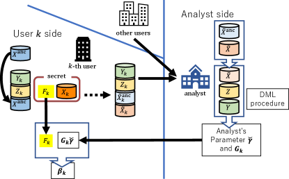
Our method DC-DML is based on DC-QE (Kawamata et al., 2024) and DML (Chernozhukov et al., 2018), and enables to estimate CATE with confidentiality preservation of distributed data. As in Kawamata et al. (Kawamata et al., 2024), DC-QE operates in two roles: user and analyst roles. Each user have confidential covariates , treatments and outcomes . DC-QE is conducted in three stages: construction of collaborative representations, estimation by the analyst, and estimation by the users. In the first stage, each user individually constructs intermediate representations and shares them with the analyst instead of the confidential dataset, then the analyst constructs the collaborative representations. In the second stage, the analyst estimates its own coefficients and variance using DML, and shares them with all users. In the final stage, each user calculates its own coefficients and variance. Each stage is described in turn from Section 4.1.1 to 4.1.3. Fig. 2 shows an overall illustration of DC-DML. Algorithm 1 is the pseudo-code of DC-DML.
4.1.1 Construction of collaborative representations
In the first stage, construction of collaborative representations, we use the aggregation method proposed in Imakura and Sakurai (Imakura and Sakurai, 2020). First, users generate and share an anchor dataset , which is a shareable dataset consisting of public or randomly constructed dummy data, where is the number of subjects in the anchor data. The anchor dataset is used to compute the transformation matrices (described below as ) required to construct the collaborative representations. Second, each user constructs intermediate representations using a linear row-wise dimensionality reduction function such as principal component analysis (PCA) (Pearson, 1901), locality preserving projection (LPP) (He and Niyogi, 2003) and factor analysis (FA) (Spearman, 1904). is consisting of a transformation matrix and a shift vector . is the reduced dimension of user . is a mean vector in with centering such as PCA and FA, or a zero vector in without centering such as LPP. Moreover, is private Note that, is a private function of user and should not be shared with other users. As will be described later in Section 4.4, the requirement that be a dimensionality reduction function and not shared with other users is important to preserve the confidentiality of the covariates. The dimensionality reduction function is applied as
where . Moreover, is private and can differ from other users. To consider the constant term in the linear CATE model, we combine to and . Formally, we can represent those as
where
Finally, each user shares the intermediate representations and , treatments and outcomes to the analyst.
Next, the analyst transforms the shared intermediate representations into an common form called collaborative representations. To do this, the analyst computes the transformation functions for all such that
where and is the dimension of collaborative representations. Then, we have the collaborative representation for as
Let
be a low-rank approximation based on singular value decomposition of the matrix combining , where is a diagonal matrix whose diagonal entries are the larger parts of the singular values and and are column orthogonal matrices whose columns are the corresponding left and right singular vectors, respectively. Matrix is then computed as
where denotes the Moore–Penrose inverse. Then, the collaborative representations are given by
4.1.2 Estimation by the analyst
In the second stage, estimation by the analyst, the analyst estimates their own CATE model based on the DML procedure that we described in Section 3. The analyst considers the data generation process as
and the linear CATE model as
where and is the collaborative representation of . The score vectors for the analyst are defined as
where and are the analyst’s functions, and is the analyst’s estimates.
The analyst’s purpose in the second stage is to obtain . To accomplish this, first, the analyst constructs and from , and using machine learning models to estimate residuals and . The estimated residuals are expressed as
Second, the analyst calculates and . is the least squares solution of the following regression equation:
That is
The analyst can calculate the variance of in (8), (9) and (10), replacing , and with , and , respectively.
4.1.3 Estimation by the users
In the final stage, estimation by the users, the users estimates their own CATE model based on parameters that the analyst returns. The analysts’s CATE model is written as
Then, for user , subject ’s estimated CATE is written as
| (11) | ||||
where
and
| (12) |
For user , is a constant term and are coefficients for in their CATE model. Thus, user ’s coefficients are expressed as .
The variance of is
Then, the variance of is
| (13) |
User can statistically test their CATE model if they obtains , and . To accomplish this, the following procedure is conducted in the final stage. First, the analyst returns and to user . Then, user calculates and as
Moreover, user calculates and using (12) and (13), respectively. Then, user obtained , and , and can test statistically .
4.2 Correctness of DC-DML
In this section, through a similar approach to Imakura et al. (Imakura et al., 2023b), we discuss the correctness of DC-DML. Now, we consider the following subspace depending on ,
where denotes the range of a matrix. Define centralized analysis (CA) as collecting and analyzing the raw data, i.e., , and , in one place. This is an ideal analysis, but not possible if the raw data contains confidential information. Then, we have Theorem 2, whose proof is in D.
Theorem 2.
Let be the coefficients, and and be functions computed in CA. Moreover, consider such that
If , , for all , and for all , then .
4.3 A dimension reduction method for DC-DML
In this section, we propose a dimensionality reduction method for DC-DML with reference to Theorem 2. The dimensionality reduction method strongly affects the performance of DC-DML. In DC-DML, the coefficients is obtained from the subspace . If we could obtain close to , we can achieve close to . To accomplish this, the subspace should contain .
Using an approach similar to Imakura et al. (Imakura et al., 2023b), we consider a dimensionality reduction method for DC-DML. Algorithm 2 is the pseudo-code of that. The basic idea of the approach is that each user constructs based on estimates of obtained from their own local dataset. The estimate of obtained by each user could be a good approximation of . Thus, a bootstrap-based method can be a reasonable choice to achieve a good subspace. Let be a parameter for sampling rate. In the bootstrap-based method, first, through the DML procedure by a random samplings of size , user obtains estimates of as . Then, user constructs , where is a vector excluding the first element of . The reason of excluding the first element of is that should be a transformation matrix for -dimensional covariates. However, since the first column of is as in (4.1.1), the subspace contains the full range that the first element of can take.
In addition, as with Imakura et al. (Imakura et al., 2023b), the subspace can be constructed by combining multiple dimensionality reduction methods. Let and be the transformation matrices of the bootstrap-based and other methods, respectively, where . Then, is
4.4 Discussion on confidentiality preservation
In this section, we discuss how DC-DML preserves the confidentiality of covariates. DC-DML prevents the original covariates from being recovered or inferred from the shared intermediate representations by the following two layers of confidentiality, inherited from DC technology (Imakura and Sakurai, 2020).
The first layer is to construct intermediate representations by dimensionality reduction of the covariates. Since the dimensionality reduction results in the loss of some of the original covariate information, it is impossible to recover the original covariates from the intermediate representations.
The second layer is that each user does not share the dimensionality reduction function with the other users. If is shared, the others can construct an approximate inverse function , and then infer the original covariates using for the shared intermediate representations of user . The construction of is possible for those who know both and , but as far as the algorithm of DC technology is followed, there is no such person except user .
Various attacks are possible to recover or infer the original covariates from the shared intermediate representations. For example, it is a collusion by users and analysts. Depending on the way of collusion, the confidentiality of the covariates may be violated, as discussed by Imakura et al. (2021a), for more details, see. However, we believe that future research could create a robust DC technology against a variety of attacks.
4.5 Advantage and disadvantage
In this section, we describe the advantages and disadvantages of DC-DML. Those are attributed to DC-QE or DML with the linear CATE model described in Section 3.
There are four advantages. First, as mentiond in Section 4.4, dimensionality reduction preserves the confidentiality of covariates. Second, since DC-DML enables to collect a larger number of subjects from distributed data, and accumulate a knowledge base, it is possible to obtain better performance than in individual analysis. Third, DC-DML does not require repetitive communication (communication-efficient). Finally, DC-DML is less susceptible to model mis-specification because it assumes a semi-parametric model.
Conversely, there are three disadvantages. First, DC-DML cannot be used directly if confidential information is included in the treatments or outcomes. Solutions to this issue include, for example, transforming treatments or outcomes into a format that preserves confidentiality through encryption and so on. Second, the performance of the resulting model may deteriorate because the dimensionality reduction reduces the information in the raw data. However, obtaining more subjects from the distributed data can improve performance more than the deterioration caused by dimensionality reduction. Finally, if the linear CATE model is not valid, i.e. non-linear, DC-DML may obtain incorrect conclusions.
5 Simulations
In this section we describe three simulations we conducted to demonstrate the effectiveness of DC-DML. 222We performed the simulations using Python codes, which are available from the corresponding author by reasonable request. In Simulation I, that uses synthetic data, we show that DC-DML is useful in the setting of data distributions that would be incorrectly estimated by individual analysis (IA), the analysis performed by the user using only their own dataset. In Simulation II, that uses semi-synthetic data generated from the infant dataset, we compare the performances between DC-DML and other existing methods. In Simulation III, that uses real-world data from the financial assets and jobs datasets, we investigate the robustness of DC-DML performance in the presence of heterogeneous numbers of subjects or treatment group proportions per party.
In Simulation II, the methods to be compared to DC-DML are as follows. First are the DMLs in IA and CA, that we denote for convenience as IA-DML and CA-DML, respectively. As described above, IA-DML and CA-DML are, respectively, targets that DC-DML should perform better and closer to. Second, GRF and X-Learner in IA and CA, denoted for convenience with the prefixes IA- and CA-: IA-GRF, CA-GRF, IA-XL, and CA-XL. Finally, the distributed data analysis methods SR and FedCI.
In the simulations, we set up the machine learning models used in DML and X-learner as follows. First, both machine learning models used to estimate and in the DML methods (IA-DML, CA-DML and DC-DML) in the Simulation I are random forests. Second, the settings of the machine learning models used in Simulations II and III are as follows. We selected the machine learning models used to estimate in the DML methods by our preliminary simulations from among five regression methods: multiple regression, random forests, K-nearest neighbor, light gradient boosting machine (LGBM) and support vector machine (SVM) with standardization. In the preliminary simulations for , we repeated the regression of the outcomes on the covariates for the candidate methods in CA setting 50 times and set the criterion of selecting the one with the smallest root mean squared errors (RMSE) average. For , similarly, we selected by preliminary simulations among five classification methods: logistic regression, random forests, K-nearest neighbor, LGBM and SVR. In our preliminary simulations for , we followed the similar procedure as for , where we set the criterion of selecting the one with the smallest average Brier score. Here, Brier Score is a mean squared error measure of probability forecasting (Brier, 1950). The hyperparameters for the candidate methods were the default values shown in E. As a result of our preliminary simulations, we chose SVM as the machine learning models to be used in the estimation of and , both in Simulation II. For the financial data set in Simulation III, we set and to multiple regression and logistic regression, respectively. For the jobs dataset, we set and to multiple regression and random forest, respectively. We use the same models for the outcome and propensity score in X-Learner (IA-XL and CA-XL) as in DML in all simulations. The results of the preliminary simulations are in F.
The settings used in DC-DML are as follows. As the intermediate representation construction methods, we used six: PCA, LPP, FA, PCA+B, LPP+B, and FA+B. Here, +B represents the combination with the bootstrap-based dimensionality reduction method. The intermediate representation dimension and collaborative representation dimension were set as for all and , respectively. In combination with the bootstrap-based dimensionality reduction method, the BS dimension was set to three in Simulation I and in Simulation II and III. Here, is the ceiling function. Anchor data were generated from uniform random numbers of maximum and minimum values for each covariate and thier subject number was the same of the original dataset .
As described below, in Simulation II, we used the five methods described in Section 2 as comparison methods: DML, GRF, X-Learner, SR and FedCI. Also, in Simulation III, we used DML and SR as comparison methods. See G for the detailed settings of those methods.
In Simulations II and III, the evaluation measures used were how close the estimates were to the benchmarks. The benchmarks in Simulations II and III were the true values and the average values of 50 trials of CA-DML, respectively. In this study, we consider four evaluation measures: the RMSE of CATE, the consistency rate of significance of CATE, the RMSE of coefficients, and the consistency rate of significance of coefficients. Note that, for simplicity of explanation, results other than the RMSE of CATE in Simulation III were shown in H.
The RMSE of CATE
The RMSE of CATE is a measure of how much the predicted CATE matched the benchmark CATE as
where is the benchmark CATE and is the estimated CATE. The lower this measure, the better.
The consistency rate of significance of CATE
The consistency rate of significance of CATE is the rate where the estimated CATE obtained a statistical test result of “significantly positive,” “significantly negative,” or “not significant” in 5% level when the benchmark CATE is positive, negative, or zero, respectively. For Simulation III, we set the benchmark CATE is positive, negative, or zero when the estimate in CA-DML is significantly positive, significantly negative or not significant, respectively, in 5% level. The higher this measure, the better. This measure was not calculated in X-Learner and FedCI, because statistical testing methods for CATE are not provided in those methods.
The RMSE of coefficients
The RMSE of coefficients is a measure of how much the estimated coefficients matched that of the benchmark as
where is the benchmark coefficient. The lower this measure, the better. Since GRF, X-Learner and FedCI are not models that estimate linear CATE, this measure was not calculated in those models.
The consistency rate of significance of coefficients
The consistency rate of significance of coefficients is the rate where the estimated coefficient obtained a statistical test result of “significantly positive,” “significantly negative,” or “not significant” in 5% level when the benchmark coefficient is positive, negative, or zero, respectively. For Simulation III, we set the benchmark coefficient is positive, negative, or zero when the estimate in CA-DML is significantly positive, significantly negative or not significant, respectively, in 5% level. The higher this measure, the better. As with the RMSE of coefficients, this measure was not calculated in GRF, X-Learner and FedCI.
5.1 Simulation I: Proof of concepts in synthetic data
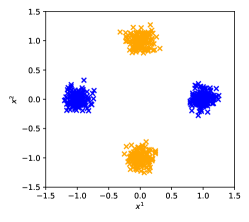
In Simulation I, we considered the situation where two parties () each had a dataset consisting of 300 subjects () and 10 covariates (). The covariates and were distributed as in Fig. 3, where blue and orange markers represent that of party 1 and 2, respectively. The other covariates were drawn from a normal distribution .
The setting of the data generation process in Simulation I was
whre w.p. is “with probability”. In this setting, the constant term and the coefficients of and should be estimated to be significantly one.
Party 1 has the dataset with the broad distribution for covariate 1 and the narrow distribution for covariate 2. Thus, party 1 would be able to estimate the coefficient of covariate 1 relatively correctly in IA-DML, but would have difficulty estimating the coefficient of covariate 2. For party 2, the opposite of party 1 can be said.
The result of Simulation I is shown in Table 2. In CA-DML, the constant term and the coefficients of and are significant and close to their true values, and the coefficients of the other covariates are not significant. Thus, CA-DML obtained reasonable estimation results. Conversely, IA-DML obtained some wrong estimation results in both parties.
| Covariates | CA-DML | IA-DML | DC-DML(PCA+B) | |||||||
|---|---|---|---|---|---|---|---|---|---|---|
| Party 1 | Party 2 | Party 1 | Party 2 | |||||||
| const. | 1.0283 | ** | 0.6300 | ** | 1.0068 | ** | 0.9563 | ** | 1.0207 | ** |
| 1.0610 | ** | 0.9952 | ** | 0.6950 | 1.0578 | ** | 1.0119 | ** | ||
| 1.1290 | ** | 2.0799 | 1.0359 | ** | 0.9042 | ** | 0.9761 | ** | ||
| -0.1628 | -0.1161 | -0.3211 | * | -0.0961 | -0.1269 | |||||
| -0.1595 | -0.0220 | -0.0021 | -0.1489 | -0.1264 | ||||||
| 0.0566 | -0.0924 | 0.1679 | 0.0147 | 0.0190 | ||||||
| 0.0905 | 0.3367 | * | -0.2482 | 0.1608 | 0.1354 | |||||
| -0.0434 | 0.0771 | -0.1849 | -0.0317 | -0.0960 | ||||||
| -0.0494 | -0.0397 | -0.1370 | -0.0336 | -0.0065 | ||||||
| 0.0607 | -0.0955 | 0.1867 | 0.0418 | 0.0536 | ||||||
| -0.1773 | -0.2022 | -0.0543 | -0.1270 | -0.1391 | ||||||
| ** , * | ||||||||||
DC-DML conducted by the PCA+B dimensionality reduction method obtained estimation results similar to CA-DML. This result suggests that even in situations where it is difficult to make valid estimates using IA-DML, DC-DML can produce more valid estimates than that.
5.2 Simulation II: Comparison with other methods in semi-synthetic data
In Simulation II, we evaluate the performance of DC-DML on semi-synthetic data generated from the infant health and development program (IHDP) dataset. The IHDP dataset is “a randomized simulation that began in 1985, targeted low-birth-weight, premature infants, and provided the treatment group with both intensive high-quality child care and home visits from a trained provider.” (Hill, 2011) 333The IHDP dataset is published as the supplementary file (https://www.tandfonline.com/doi/abs/10.1198/jcgs.2010.08162). The IHDP dataset is consisting of 25 covariates and a treatment variable and does not include an outcome variable. Thus, the outcomes needs to be synthetically set up for the simulation. Hill Hill (2011) removed data on all children with nonwhite mothers from the treatment group to imbalance the covariates in the treatment and control groups. We followed this as well, and as a result, the dataset in Simulation II consisted of 139 subjects in the treatment group and 608 subjects in the control group.
In Simulation II, we considered the situation where three parties () each had a dataset consisting of 249 subjects () and 25 covariates (). The ratios of treatment groups were equal in all parties. The outcome variable in Simulation II we set as
| const. | |||
where and are the average of and standard deviation of covariate , respectively, in the dataset. Note that, and were not defined because the treatments were included in the dataset.
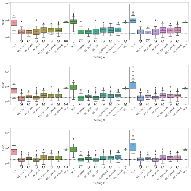
The results of the four evaluation measures in Simulation II is shown in Fig. 4-4. In this simulation, we conducted 50 simulations with different random seed values for data distributing and machine learning. The symbols and in parentheses in the figures represent significant positive and significant negative differences from the IA-DML results, respectively, in -test. There were no methods that were not significantly different from DC-DML.
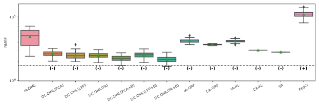
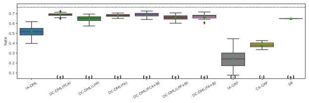
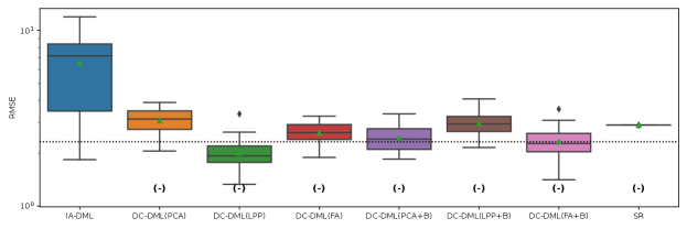
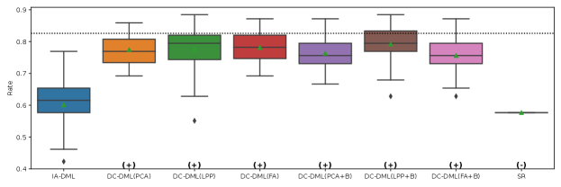
As described below, Fig. 4-4 show that DC-DML performs well for each of the evaluation measures in Simulation 2. First, as shown in Fig. 4, the result for the RMSE of CATE shows that DC-DML significantly outperformed IA-DML. Moreover, DC-DML obtained better result than the existing methods. Second, as shown in Fig. 4, the result for the consistency rate of significance of CATE shows that DC-DML significantly outperformed IA-DML. Moreover, DC-DML obtained better result than the existing methods. Third, as shown in Fig. 4, the result for the RMSE of coefficients shows that DC-DML significantly outperformed IA-DML and are comparable to CA-DML and SR. Finally, as shown in Fig. 4, the result for the consistency rate of significance of coefficients shows that DC-DML significantly outperformed IA-DML. Moreover, DC-DML obtained better result than SR. These results in Simulation II suggests that DC-DML can outperform IA-DML and obtain equal or better results than the existing methods.
5.3 Simulation III: Robustness to distribution settings in real-world data
Based on real-world datasets of financial assets and jobs, in Simulation III, we investigate the robustness of DC-DML performance in the case where the number of subjects or rate of treatment group across parties is imbalanced. As the financial assets dataset, we focused on the survey of income and program participation (SIPP) dataset, which was used in Chernozhukov et al. (Chernozhukov et al., 2018) to estimate the effect of 401(k) eligibility on accumulated assets. 444This is avaiable from the repository of Chernozhukov et al. (2018) (https://github.com/VC2015/DMLonGitHub/). The SIPP dataset consists of 9915 observations and includes nine subject information (age, inc, educ, fsize, marr, twoearn, db, pira, hown) as covariates, 401(k) offerings as treatments, and net financial assets as outcomes. As the jobs dataset, we focused on Dehejia and Wahba’s dataset (Dehejia and Wahba, 1999), which was used to estimate the treatment effects of work experience and counseling on incomes. 555This is avaiable from the author’s website (https://users.nber.org/~rdehejia/nswdata.html). The jobs dataset consists of 2675 observations and includes eight subject information (age, black, hispanic, married, no degree, re74) as covariates, trainings as treatments, and real earnings in 1978 as outcomes.
In Simulation III, we considered three parties () and three settings for data distribution where the rate of treatment group and the number of subjects are even or uneven, as shown in Table 3. In setting A, all parties have the same number of subjects and the same rate of treatment groups. In setting B, the number of subjects is even, but the rate of treatment groups differs across parties. In setting C, the number of subjects differs, but the rate of treatment groups is even across parties.
| setting A | setting B | setting C | ||||||||
| subjects | even | even | uneven | |||||||
| treatment rate | even | uneven | even | |||||||
| dataset | party | all | treated | controlled | all | treated | controlled | all | treated | controlled |
| financial assets | 1 | 3304 | 1227 | 2077 | 3304 | 2549 | 755 | 6864 | 2549 | 4315 |
| 2 | 3304 | 1227 | 2077 | 3304 | 849 | 2455 | 2287 | 849 | 1438 | |
| 3 | 3304 | 1227 | 2077 | 3304 | 283 | 3021 | 762 | 283 | 479 | |
| jobs | 1 | 891 | 61 | 830 | 891 | 92 | 799 | 1337 | 92 | 1245 |
| 2 | 891 | 61 | 830 | 891 | 61 | 830 | 891 | 61 | 830 | |
| 3 | 891 | 61 | 830 | 891 | 30 | 861 | 445 | 30 | 415 | |
In Simulation III, the result of CA-DML is used as the benchmark. Table 4 shows the average results of 50 trials of CA-DML. Note that, comparisons with GRF, X-Learner, and FedCI do not make sense because those assume the non-linear CATE model. Thus, only CA-DML, IA-DML and SR were considered as comparison with DC-DML.
| financial assets | jobs | ||||
|---|---|---|---|---|---|
| covariate | coefficient | covariate | coefficient | ||
| const. | -9705.1794 | const. | -7533.7519 | ||
| age | 172.0307 | age | 226.4912 | * | |
| inc | -0.1297 | black | 2493.7939 | ||
| educ | 642.9040 | hispanic | 1519.3141 | ||
| fsize | -1003.0686 | married | -2215.7011 | ||
| marr | 1102.9090 | no_degree | -858.5624 | ||
| twoearn | 5607.3989 | re74 | -0.3354 | ||
| db | 5657.7264 | * | |||
| pira | -1032.3599 | ||||
| hown | 5324.2854 | * | |||
| * | |||||
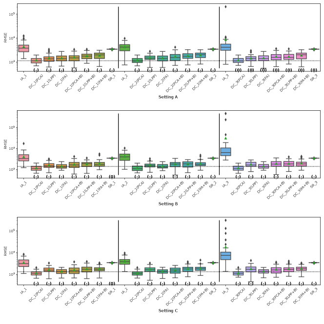
Fig. 5 represents the RMSE of CATE in Simulation III for the financial assets dataset. The symbols , and 0 in parentheses in the figures represent significant positive, significant negative and not significant differences from the IA-DML results, respectively, in -test. The results for parties 1, 2 and 3 are shown on the left, middle and right sides, respectively, in the figures. In all cases shown in Fig. 5, DC-DML results are better than IA-DML and SR. In addition, the dimensionality reduction method combined with bootstrapping shows robust results. However, DC-DML using LPP are relatively worse than for DC-DML using the other dimensionality reduction methods. No SR results are better than IA-DML.
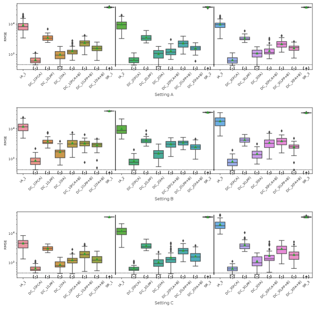
Fig. 6 represents the RMSE of CATE in Simulation III for the jobs dataset. Similar to the simulation for the financial assets, DC-DML results are better than IA-DML and SR in all cases in Fig. 6. Although, as shown in H, DC-DML does not always exhibits better performance than IA-DML in the other measures, DC-DML results are often better than IA-DML. As with the financial assets dataset, the dimensionality reduction method combined with bootstrapping shows robust results, and SR results are often worse than IA-DML.
The simulation results in both datasets suggest that the choice of dimensionality reduction method has a significant impact on the performance of DC-DML. What dimensionality reduction method provides good performance for DC-DML is likely to be data-dependent. How to select a dimensionality reduction method is a future issue.
On summary, in Simulation III with two datasets, DC-DML achieved better results than IA-DML, although not in all cases. Those results suggest that DC-DML can obtain comparable results to CA-DML in various data distribution settings than in IA-DML.
6 Discussion
Utilizing distributed data across multiple parties is a important topic in data science, but confidential or privacy concerns need to be addressed. Multi-source data fusion to construct models for the estimation of CATE can help to provide better policy or medical treatments for subjects. Our method provides statistical test results for treatment effects. This allows us to make decisions such as applying the treatment only to subjects with significantly better effects, or discontinuing the treatment for subjects with significantly worse effects. Giving procedures that take into account the subjects’s covariates is essential for safer and more efficient policy and health care implementation.
Our method enables the collaborative representation to be constructed again for each additional collaboration party. In addition, our method requires communication with the analyst only at the time of sharing intermediate representations or receiving estimation results, and does not require long time synchronization. This advantage enables intermediate representations to be accumulated over a longer time involving a larger number of parties, and then CATE can be estimated in refined models with large accumulated data, i.e. knowledge base.
Here, we briefly discuss the relationship between the readily identifiability, an important issue in privacy preservation literature, and our method. In the DC analysis literature, the readily identifiability indicates that the original data containing privacy information can be readily identified with the intermediate representation (Imakura et al., 2023a). Solving the readily identifiability issue could enhance the privacy preservation of our method. As shown in I, our method can be extended to use intermediate representations that are not readily identifiable with the original data. For more detailed discussion for the readily identifiability, see I.
Our study has some limitations. First, our method assumes the linear CATE model. As mentiond in Section 4.5, the linear CATE model may obtain incorrect conclusions in data where the assumption is not valid. Second, it is not clear how the dimensionality reduction method should be selected in DC-DML. Addressing these issues is a future study.
7 Conclusion
In this study, we proposed DC-DML, which estimates CATEs from privacy-preserving fusion data constructed from distributed data. Our method enables flexible estimation of CATE models from fusion data through a semi-parametric approach and does not require iterative communication. Moreover, our method enables collaborative estimation between multiple time points and different parties through the accumulation of a knowledge base. These are important characteristics with application to the practical use of our methods. Through the three simulations, we demonstrated the effectiveness of our method as follows. First, even in situations where it is difficult to make valid estimates using IA-DML, DC-DML can produce more valid estimates than that. Second, DC-DML can outperform IA-DML and obtain equal or better results than the existing methods. Third, DC-DML can obtain comparable results to CA-DML in various data distribution settings than in IA-DML.
In the future, we will develop our model to address nonlinear CATE models. Other directions include the development of our method to address vertically distributed data, and experiments in application to marketing datasets.
Acknowledgement
The authors gratefully acknowledge the New Energy and Industrial Technology Development Organization (NEDO) (No. JPNP18010), Japan Science and Technology Agency (JST) (No. JPMJPF2017), Japan Society for the Promotion of Science (JSPS), and Grants-in-Aid for Scientific Research (Nos. JP19KK0255, JP21H03451, JP23K22166, JP22K19767).
Appendix A Acronym table
A list of acronyms and definitions used in this paper is shown in Table 5.
| Acronym | Definition |
|---|---|
| AIPW | Augmented inverse propensity weighted |
| ATE | Average treatment effect |
| CA | Centralized analysis |
| CATE | Conditional average treatment effect |
| DC | Data collaboration |
| DC-DML | Data collaboration double machine learning |
| DC-QE | Data collaboration quasi-experiment |
| DML | Double machine learning |
| FA | Factor analysis |
| FedCI | Federated causal inference |
| GRF | Generalized random forest |
| IA | Individual analysis |
| IHDP | Infant health and development program |
| IPW | Inverse propensity-weighted |
| LGBM | Light gradient boosting machine |
| LPP | Locality preserving projection |
| MLE | Maximum likelihood estimator |
| PCA | Principal component analysis |
| RMSE | Root mean squared error |
| SIPP | Survey of income and program participation |
| SR | Secure regression |
| SVM | Support vector machine |
Appendix B Algorithm of data collaboration quasi-experiment
Algorithm 3 is the pseudo-code of data collaboration quasi-experiment (DC-QE).
Appendix C The proof of Theorem 1
Proof.
Denote . First, we can prove the moment condition as
Second, for the Neyman–orthogonality, consider
where and . Then,
Here,
The first term is
and the second term is
Thus,
∎
Appendix D The proof of Theorem 2
Proof.
From Theorem 1 in Imakura et al. (2021a), if
then we have
where . Denote as the th row of . Here, consider
then, we can express . Since ,
Thus, is equal to the solution of the following least squares problem:
From the assumption ,
We used the assumptions and to transform the equation from line 2 to 3. It is obvious that and are equal in all but the first element. However,
where is the first element of . Then, . ∎
Appendix E Hyperparameters for candidate methods
Most hyperparameters of candidate methods for and are default parameters in scikit-learn (V1.2.2) and LightGBM (V3.3.5). The hyperparameters for estimation are as follows.
- LinearRegression (scikit-learn)
-
fit_intercept: True, positive: False
- RandomForestRegressor (scikit-learn)
-
bootstrap: True, ccp_alpha: 0.0, criterion: squared_error, max_depth: None, max_features: 1.0, max_leaf_nodes: None, max_samples: None, min_impurity_decrease: 0.0, min_samples_leaf: 1, min_samples_split: 2, min_weight_fraction_leaf: 0.0, n_estimators: 100, oob_score: False, warm_start: False
- KNeighborsRegressor (scikit-learn)
-
algorithm: auto, leaf_size: 30, metric: minkowski, metric_params: None, n_neighbors: 5, p: 2, weights: uniform
- LGBMRegressor (LightGBM)
-
boosting_type: gbdt, class_weight: None, colsample_bytree: 1.0, importance_type: split, learning_rate: 0.1, max_depth: -1, min_child_samples: 20, min_child_weight: 0.001, min_split_gain: 0.0, n_estimators: 100, num_leaves: 31, objective: None, reg_alpha: 0.0, reg_lambda: 0.0, subsample: 1.0, subsample_for_bin: 200000, subsample_freq: 0
- SVR (scikit-learn)
-
C: 1.0, cache_size: 200, coef0: 0.0, degree: 3, epsilon: 0.1, gamma: scale, kernel: rbf, max_iter: -1, shrinking: True, tol: 0.001
The hyperparameters for estimation are as follows.
- LogisticRegression (scikit-learn)
-
C: 1.0, class_weight: None, dual: False, fit_intercept: False, intercept_scaling: 1, l1_ratio: None, max_iter: 100, multi_class: auto, n_jobs: None, penalty: none, solver: lbfgs, tol: 0.0001, warm_start: False
- RandomForestClassifier (scikit-learn)
-
bootstrap: True, ccp_alpha: 0.0, class_weight: None, criterion: gini, max_depth: None, max_features: sqrt, max_leaf_nodes: None, max_samples: None, min_impurity_decrease: 0.0, min_samples_leaf: 1, min_samples_split: 2, min_weight_fraction_leaf: 0.0, n_estimators: 100, oob_score: False, warm_start: False
- KNeighborsClassifier (scikit-learn)
-
algorithm: auto, leaf_size: 30, metric: minkowski, metric_params: None, n_neighbors: 5, p: 2, weights: uniform
- LGBMClassifier (LightGBM)
-
boosting_type: gbdt, class_weight: None, colsample_bytree: 1.0, importance_type: split, learning_rate: 0.1, max_depth: -1, min_child_samples: 20, min_child_weight: 0.001, min_split_gain: 0.0, n_estimators: 100, num_leaves: 31, objective: None, reg_alpha: 0.0, reg_lambda: 0.0, subsample: 1.0, subsample_for_bin: 200000, subsample_freq: 0
- SVC (scikit-learn)
-
C: 1.0, break_ties: False, cache_size: 200, class_weight: None, coef0: 0.0, decision_function_shape: ovr, degree: 3, gamma: scale, kernel: rbf, max_iter: -1, probability: True, shrinking: True, tol: 0.001
Appendix F The results of the preliminary simulations
In the preliminary simulations, RMSE was calculated for the estimation of and Brier score for the estimation of using a two folds cross-validation with raw data. Table 6 shows the averages of 50 trials.
| Simulation II | |||
|---|---|---|---|
| RMSE | Brier score | ||
| Multiple regression | 2.5613 | Logistic regression | 0.2579 |
| Random forests | 2.5308 | Random forests | 0.1532 |
| K-nearest neighbor | 2.8690 | K-nearest neighbor | 0.1665 |
| LGBM | 2.5734 | LGBM | 0.1733 |
| SVM | 2.2333 | SVM | 0.1488 |
| Simulation III for the financial assets dataset | |||
| RMSE | Brier score | ||
| Multiple regression | 55827.4190 | Logistic regression | 0.2014 |
| Random forests | 58048.7840 | Random forests | 0.2151 |
| K-nearest neighbor | 57861.6099 | K-nearest neighbor | 0.2339 |
| LGBM | 56665.7031 | LGBM | 0.2047 |
| SVM | 65450.8516 | SVM | 0.2080 |
| Simulation III for the jobs dataset | |||
| RMSE | Brier score | ||
| Multiple regression | 10963.5250 | Logistic regression | 0.1699 |
| Random forests | 12058.0681 | Random forests | 0.1628 |
| K-nearest neighbor | 11981.2699 | K-nearest neighbor | 0.1751 |
| LGBM | 11503.7386 | LGBM | 0.1719 |
| SVM | 15613.6765 | SVM | 0.1912 |
Appendix G Settings for the existing methods
To conduct the exsting method, we used EconML (V0.14.1) and FedCI (https://github.com/vothanhvinh/FedCI). All hyperparameters of GRF (CausalForest) and FedCI are default values as follows.
- CausalForest (EconML)
-
criterion: mse, fit_intercept: True, honest: True, inference: True, max_depth: None, max_features: auto, max_samples: 0.45, min_balancedness_tol: 0.45, min_impurity_decrease: 0.0, min_samples_leaf: 5, min_samples_split: 10, min_var_fraction_leaf: None, min_var_leaf_on_val: False, min_weight_fraction_leaf: 0.0, n_estimators: 100, subforest_size: 4, warm_start: False
- FedCI
-
n_iterations:2000, learning_rate:1e-3
For X-Learner, candidate methods for estimation of the outcome and propensity score have the hyperparameters described in E. For SR, we considered the regression model to consist of a constant term and a cross term between the covariates and the treatment as
Appendix H The all results of Simulation III
In this section, we include all results of Simulation III.
Fig. 5, 7, 8 and 9 represent the results of Simulation III for the financial assets dataset. In the RMSE of coefficients and the consistency rate of significance of coefficients shown in Fig. 8 and 9, DC-DML results for party1 using LPP are worse than for IA-DML in some cases. However, in most other cases shown in Fig. 5, 7, 8 and 9, DC-DML results are better than IA-DML. In addition, the dimensionality reduction method combined with bootstrapping shows robust results. No SR results are better than IA-DML.
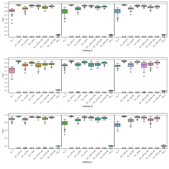
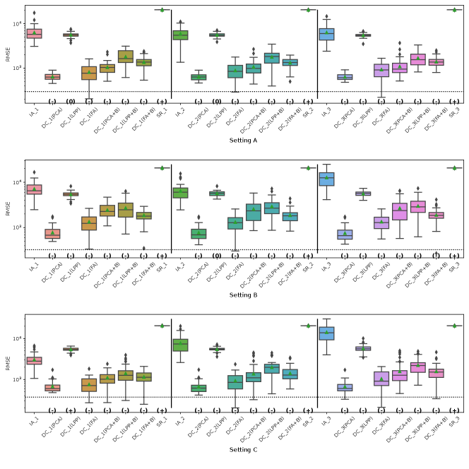
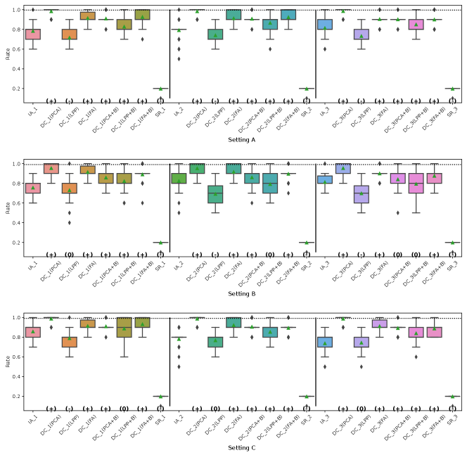
Fig. 6, 10, 11 and 12 represent the results of Simulation III for the jobs dataset. DC-DML results are worse than IA-DML when using LPP for the consistency rate of significance of CATE, and using LPP, LPP+B or FA+B for the consistency rate of significance of coefficients. However, DC-DML results are often better than IA-DML. DC-DML performs better than IA-DML particularly in the RMSEs of CATE and coefficients in most cases. Moreover, as with the financial assets dataset, the dimensionality reduction method combined with bootstrapping shows robust results. SR results are often worse than IA-DML.
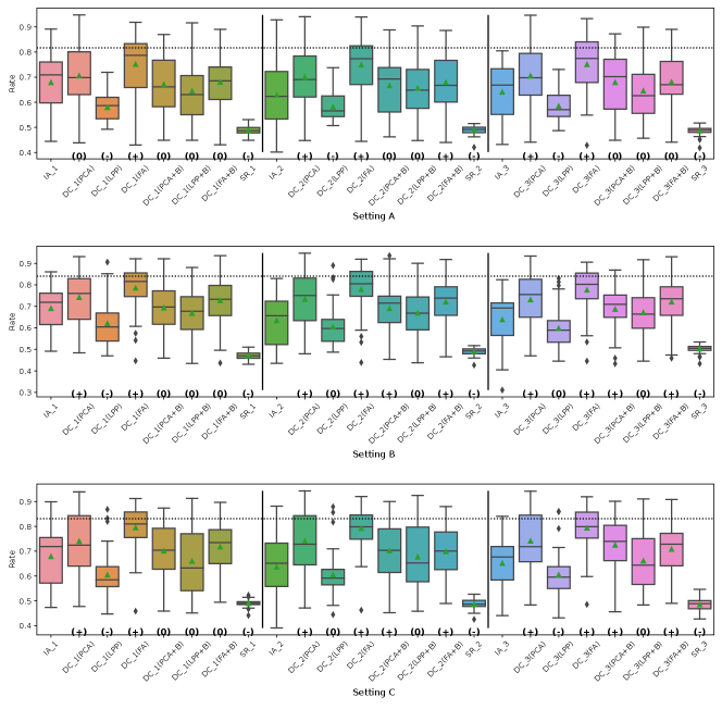
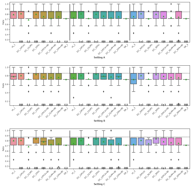
On both datasets, there were cases where better performance was not achieved with DC-DML using LPP, especially. This suggests that the choice of dimensionality reduction method has a significant impact on the performance of DC-DML.
Appendix I Non-readily identifiable method
The definition of the readily identifiability (Imakura et al., 2023a) is the following.
Definition 1.
Let and be a pair of the data including and not including personal information that can directly identify a specific subject for the th person, respectively. We let and be personal information and non-personal information datasets for the same persons, respectively.
For non-personal information , if and only if someone else holds a key to correctly collate the corresponding personal information or can generate the key by their own, then the non-personal dataset is defined as “readily identifiable” to personal dataset .
Imakura et al. (Imakura et al., 2023a) showed that the intermediate representation is readily identifiable to the original dataset in DC analysis. This is also true for DC-DML, i.e., is readily identifiable to .
To solve readily identifiable issue in DC analysis, Imakura et al. (Imakura et al., 2023a) proposed strategies in which the intermediate representations are non-readily identifiable to the original dataset. To develop DC-DML not to be readily identifiable, the following strategies are needed.
-
•
The sample indices in each user are permuted randomly.
-
•
Dimensionality reduction functions are erasable and cannot be reconstructed.
According to the above strategies, we develop DC-DML as a non-readily identifiable DC-DML (NI-DC-DML) as follows. In the second stage, construction of collaborative representations, there are three different procedures between DC-DML and NI-DC-DML. First, in NI-DC-DML, user constructs instead of as dimensionality reduction function, where is a random matrix. Second, user constructs a permutation matrix . Thus, the intermediate representations are constructed as
Note that, is not applied for construction of . Then, user erases and . and cannot be reconstructed if random number generator with different random seed for each user is used. Third, user shares permutated treatments and outcomes , instead of and , respectively, to the analyst. Then, user erases , , and .
In the final stage, estimation of the users, there are two different procedures between DC-DML and NI-DC-DML. First, the analyst returns and instead of and , respectively, where
Second, user calculates and as
The above calculation is correct because
The other procedures in NI-DC-DML are the same as in DC-DML. Algorithm 4 is the pseudo-code of NI-DC-DML.
The estimation result obtained in NI-DC-DML when is the identity matrix is equal to that obtained in DC-DML. Conversely, if is not the identity matrix, the NI-DC-DML and DC-DML estimation results differ. However, we think the difference is not large. As an example, we show in Table 7 the estimation results of NI-DC-DML in the situation of Simulation I. The results are correct except that the coefficient of for party 2 is significant.
Strictly, if or are continuous values, NI-DC-DML cannot satisfy the non-readily identifiability. The solution to this issue could be the use of other privacy preservation technologies such as -anonymization, differential privacy or cryptography. That is one of the important future issues. Further investigation of the relationship between the readily identifiability and DC-DML deviates significantly from the purpose of this paper, thus we end our discussion here.
| Covariates | DC-DML(PCA+B) | |||
|---|---|---|---|---|
| Party 1 | Party 2 | |||
| const. | 0.9133 | ** | 0.9772 | ** |
| 1.0451 | ** | 0.9593 | ** | |
| 0.8847 | ** | 1.0420 | ** | |
| -0.1566 | -0.2426 | * | ||
| -0.0559 | 0.0028 | |||
| 0.0189 | 0.0158 | |||
| 0.1160 | 0.0359 | |||
| 0.0598 | -0.1224 | |||
| -0.0413 | 0.0371 | |||
| 0.0492 | 0.0802 | |||
| -0.1166 | -0.1608 | |||
| ** , * | ||||
References
- Athey et al. (2019) S. Athey, J. Tibshirani, and S. Wager. Generalized random forests. The Annals of Statistics, 47(2):1148, 2019.
- Bia et al. (2023) M. Bia, M. Huber, and L. Lafférs. Double machine learning for sample selection models. Journal of Business & Economic Statistics, pages 1–12, 2023.
- Bogdanova et al. (2020) A. Bogdanova, A. Nakai, Y. Okada, A. Imakura, and T. Sakurai. Federated learning system without model sharing through integration of dimensional reduced data representations. In Proceedings of IJCAI 2020 International Workshop on Federated Learning for User Privacy and Data Confidentiality, 2020.
- Brier (1950) G. W. Brier. Verification of forecasts expressed in terms of probability. Monthly weather review, 78(1):1–3, 1950.
- Chernozhukov et al. (2018) V. Chernozhukov, D. Chetverikov, M. Demirer, E. Duflo, C. Hansen, W. Newey, and J. Robins. Double/debiased machine learning for treatment and structural parameters. The Econometrics Journal, 21(1):C1–C68, 01 2018. ISSN 1368-4221. doi: 10.1111/ectj.12097. URL https://doi.org/10.1111/ectj.12097.
- Criado et al. (2022) M. F. Criado, F. E. Casado, R. Iglesias, C. V. Regueiro, and S. Barro. Non-iid data and continual learning processes in federated learning: A long road ahead. Information Fusion, 88:263–280, 2022.
- Dehejia and Wahba (1999) R. H. Dehejia and S. Wahba. Causal effects in nonexperimental studies: Reevaluating the evaluation of training programs. Journal of the American statistical Association, 94(448):1053–1062, 1999.
- Engle et al. (1986) R. F. Engle, C. W. J. Granger, J. Rice, and A. Weiss. Semiparametric estimates of the relation between weather and electricity sales. Journal of the American statistical Association, 81(394):310–320, 1986.
- Fan et al. (2022) Q. Fan, Y. Hsu, R. P. Lieli, and Y. Zhang. Estimation of conditional average treatment effects with high-dimensional data. Journal of Business & Economic Statistics, 40(1):313–327, 2022.
- He and Niyogi (2003) X. He and P. Niyogi. Locality preserving projections. Advances in neural information processing systems, 16, 2003.
- Hill (2011) J. L. Hill. Bayesian nonparametric modeling for causal inference. Journal of Computational and Graphical Statistics, 20(1):217–240, 2011.
- Imakura and Sakurai (2020) A. Imakura and T. Sakurai. Data collaboration analysis framework using centralization of individual intermediate representations for distributed data sets. ASCE-ASME Journal of Risk and Uncertainty in Engineering Systems, Part A: Civil Engineering, 6(2):04020018, 2020.
- Imakura et al. (2021a) A. Imakura, A. Bogdanova, T. Yamazoe, K. Omote, and T. Sakurai. Accuracy and privacy evaluations of collaborative data analysis. In The Second AAAI Workshop on Privacy-Preserving Artificial Intelligence (PPAI-21), 2021a.
- Imakura et al. (2021b) A. Imakura, H. Inaba, Y. Okada, and T. Sakurai. Interpretable collaborative data analysis on distributed data. Expert Systems with Applications, 177:114891, 2021b.
- Imakura et al. (2023a) A. Imakura, T. Sakurai, Y. Okada, T. Fujii, T. Sakamoto, and H. Abe. Non-readily identifiable data collaboration analysis for multiple datasets including personal information. Information Fusion, 98:101826, 2023a.
- Imakura et al. (2023b) A. Imakura, R. Tsunoda, R. Kagawa, K. Yamagata, and T. Sakurai. DC-COX: Data collaboration cox proportional hazards model for privacy-preserving survival analysis on multiple parties. Journal of Biomedical Informatics, 137:104264, 2023b.
- Imbens and Rubin (2015) G. W. Imbens and D. B. Rubin. Causal inference in statistics, social, and biomedical sciences. Cambridge University Press, 2015.
- Karr et al. (2005) A. F. Karr, X. Lin, A. P. Sanil, and J. P. Reiter. Secure regression on distributed databases. Journal of Computational and Graphical Statistics, 14(2):263–279, 2005.
- Kawamata et al. (2024) Y. Kawamata, R. Motai, Y. Okada, A. Imakura, and T. Sakurai. Collaborative causal inference on distributed data. Expert Systems with Applications, 244:123024, 2024.
- Konečnỳ et al. (2016) J. Konečnỳ, H. B. McMahan, F. X. Yu, P. Richtárik, A. T. Suresh, and D. Bacon. Federated learning: Strategies for improving communication efficiency. In NIPS Workshop on Private Multi-Party Machine Learning, 2016. URL https://arxiv.org/abs/1610.05492.
- Künzel et al. (2019) S. R. Künzel, J. S. Sekhon, P. J. Bickel, and B. Yu. Metalearners for estimating heterogeneous treatment effects using machine learning. Proceedings of the national academy of sciences, 116(10):4156–4165, 2019.
- McMahan et al. (2017) B. McMahan, E. Moore, D. Ramage, S. Hampson, and B. A. y Arcas. Communication-efficient learning of deep networks from decentralized data. In Artificial intelligence and statistics, pages 1273–1282. PMLR, 2017.
- Pearson (1901) K. Pearson. LIII. on lines and planes of closest fit to systems of points in space. The London, Edinburgh, and Dublin philosophical magazine and journal of science, 2(11):559–572, 1901.
- Rafi et al. (2024) T. H. Rafi, F. A. Noor, T. Hussain, and D. Chae. Fairness and privacy preserving in federated learning: A survey. Information Fusion, 105:102198, 2024.
- Rodríguez-Barroso et al. (2020) N. Rodríguez-Barroso, G. Stipcich, D. Jiménez-López, J. A. Ruiz-Millán, E. Martínez-Cámara, G. González-Seco, M. V. Luzón, M. A. Veganzones, and F. Herrera. Federated learning and differential privacy: Software tools analysis, the sherpa. ai fl framework and methodological guidelines for preserving data privacy. Information Fusion, 64:270–292, 2020.
- Rodríguez-Barroso et al. (2023) N. Rodríguez-Barroso, D. Jiménez-López, M. V. Luzón, F. Herrera, and E. Martínez-Cámara. Survey on federated learning threats: Concepts, taxonomy on attacks and defences, experimental study and challenges. Information Fusion, 90:148–173, 2023.
- Rolling et al. (2019) C. A. Rolling, Y. Yang, and D. Velez. Combining estimates of conditional treatment effects. Econometric Theory, 35(6):1089–1110, 2019.
- Rosenbaum and Rubin (1983) P. R. Rosenbaum and D. B. Rubin. The central role of the propensity score in observational studies for causal effects. Biometrika, 70(1):41–55, 1983.
- Shi et al. (2024) P. Shi, X. Zhang, and W. Zhong. Estimating conditional average treatment effects with heteroscedasticity by model averaging and matching. Economics Letters, 238:111679, 2024.
- Spearman (1904) C. Spearman. “general intelligence,” objectively determined and measured. The American Journal of Psychology, 15(2):201–292, 1904.
- Taddy et al. (2016) M. Taddy, M. Gardner, L. Chen, and D. Draper. A nonparametric bayesian analysis of heterogenous treatment effects in digital experimentation. Journal of Business & Economic Statistics, 34(4):661–672, 2016.
- Tan et al. (2022) X. Tan, C. H. Chang, L. Zhou, and L. Tang. A tree-based model averaging approach for personalized treatment effect estimation from heterogeneous data sources. In International Conference on Machine Learning, pages 21013–21036. PMLR, 2022.
- Vo et al. (2022) T. V. Vo, Y. Lee, T. N. Hoang, and T.-Y. Leong. Bayesian federated estimation of causal effects from observational data. In The 38th Conference on Uncertainty in Artificial Intelligence, 2022. URL https://openreview.net/forum?id=BEl3vP8sqlc.
- Xiong et al. (2023) R. Xiong, A. Koenecke, M. Powell, Z. Shen, J. T. Vogelstein, and S. Athey. Federated causal inference in heterogeneous observational data. Statistics in Medicine, 42(24):4418–4439, 2023.