Estimation of the size and structure of the broad line region using Bayesian approach

Amit Kumar Mandal^1,2, Suvendu Rakshit^3,4, C. S. Stalin², R. G. Petrov⁵, Blesson Mathew¹, Ram Sagar²

¹Department of Physics, CHRIST (Deemed to be University), Hosur Road, Bangalore 560 029, India
²Indian Institute of Astrophysics, Block II, Koramangala, Bangalore, 560 034, India
³Aryabhatta Research Institute of Observational Sciences, Manora Peak, Nainital 263002, India
⁴Finnish Centre for Astronomy with ESO (FINCA), University of Turku, Quantum, Vesilinnantie 5, 20014 University of Turku, Finland
⁵Observatoire de la C

\hat{o}

te d’Azur, CNRS, Laboratoire Lagrange, Universit

\acute{e}

\hat{o}

te d’Azur, Parc Valrose, B

\hat{a}

t. H. Fizeau, F-06108 Nice, France

E-mail: amitkumar@iiap.res.in

(Accepted 2020 December 30. Received 2020 December 28; in original form 2019 November 20)

Abstract

Understanding the geometry and kinematics of the broad line region (BLR) of active galactic nuclei (AGN) is important to estimate black hole masses in AGN and study the accretion process. The technique of reverberation mapping (RM) has provided estimates of BLR size for more than 100 AGN now, however, the structure of the BLR has been studied for only a handful number of objects. Towards this, we investigated the geometry of the BLR for a large sample of 57 AGN using archival RM data. We performed systematic modeling of the continuum and emission line light curves using a Markov Chain Monte Carlo method based on Bayesian statistics implemented in PBMAP (Parallel Bayesian code for reverberation $-$ MAPping data) code to constrain BLR geometrical parameters and recover velocity integrated transfer function. We found that the recovered transfer functions have various shapes such as single-peaked, double-peaked and top-hat suggesting that AGN have very different BLR geometries. Our model lags are in general consistent with that estimated using the conventional cross-correlation methods. The BLR sizes obtained from our modeling approach is related to the luminosity with a slope of $0.583\pm 0.026$ and $0.471\pm 0.084$ based on H $\beta$ and H $\alpha$ lines, respectively. We found a non-linear response of emission line fluxes to the ionizing optical continuum for 93 $\%$ objects. The estimated virial factors for the AGN studied in this work range from 0.79 to 4.94 having a mean at $1.78\pm 1.77$ consistent with the values found in the literature.

keywords:

galaxies: active

-

galaxies: Seyfert

-

(galaxies:) model: Bayesian

^†^†pubyear: 2020^†^†pagerange: Estimation of the size and structure of the broad line region using Bayesian approach–B

1 Introduction

Active Galactic Nuclei (AGN) are believed to be powered by the accretion of matter on to super massive black hole (SMBH; 10⁶ $-$ 10¹⁰ M_⊙) located at the center of galaxies (Lynden-Bell, 1969; Salpeter, 1964). This extreme physical process is responsible for the radiation we receive from AGN over a wide range of energies predominantly emitted in X-ray, UV and optical wavelengths. The SMBH is surrounded by the accretion disk and the optical/UV emission seen in the spectral energy distribution of an AGN is attributed to the thermal emission from the accretion disk. Farther from the accretion disk on scales of about $\sim$ 0.01 parsec (typical for the Seyfert galaxies category of AGN) lies the broad line region (BLR) that produces the line emission. The UV/optical continuum from the accretion disk photoionizes the gas clouds in the BLR, and as these gas clouds are situated deep within the potential well of the black hole, the emission lines from them are broadened by few thousands of km/sec. The BLR is surrounded by the dusty torus which is responsible for the different manifestations of the AGN when viewed at different orientations (Antonucci, 1993; Urry & Padovani, 1995). According to Barvainis (1987), the bump or excess in the near infrared (NIR) continuum is thermally produced by the hot dust grains heated by the UV/optical radiation from the central region. For a typical UV luminosity of $10^{42}-10^{44}$ $\mathrm{erg~{}s^{-1}}$ , the inner extent of the torus is around $0.01-0.1$ pc or $10-100$ light-days (Suganuma et al., 2006). Thus, the central region of AGN is highly compact, and difficult to probe using any current imaging techniques. However, recently, from interferometric observations carried out in IR using the GRAVITY instrument on the European Very Large Telescope (VLT), Gravity Collaboration et al. (2018) were able to resolve the central region in 3C 273 on scales of about 0.12 parsec. On much larger scales in AGN are the clouds in the narrow line region that are responsible for the narrow emission lines we see in the spectrum of AGN with widths of few hundreds of km/sec.

One of the defining characteristics of AGN is that they show flux variations (Wagner & Witzel, 1995; Ulrich et al., 1997). This is known since their discovery, though, the causes of flux variations are not yet understood. In spite of that, the flux variability characteristic of AGN provides a very useful way to probe the spatially unresolved inner regions in them. A technique that uses the variability of AGN to probe their central regions is known as reverberation mapping (RM; Blandford & McKee, 1982; Peterson, 1993). This method is based on the variation of the line-fluxes from the BLR in response to the the continuum UV-optical flux variations from the accretion disk. The time delay ( $\tau$ ) measured using the traditional cross-correlation techniques (Edelson & Krolik 1988; Peterson 1993) between the continuum flux and line flux variations is the average light travel time from the accretion disk to the BLR, which in principle gives the average radius of the BLR. Having the BLR size ( $R_{\mathrm{BLR}}=\tau/c$ , where c is the velocity of light) and the width of the broad emission line ( $\Delta V$ ), measurable from the spectrum, the mass of the black hole (M_BH) in an AGN can be estimated using the virial relation,

\displaystyle M_{\mathrm{BH}}=f_{\mathrm{BLR}}\left(\frac{\Delta V^{2}R_{\mathrm{BLR}}}{G}\right)

(1)

where $G$ represents the gravitational constant and $f_{\mathrm{BLR}}$ is the virial factor that depends on the geometry and kinematics of BLR. The method of RM has been used to measure M_BH in more than 100 AGN with most of the measurements coming from the compilation¹¹1http://www.astro.gsu.edu/AGNmass/ of Bentz & Katz (2015), the Sloan Digital Sky Survey Reveberation Measurement project; SDSS $-$ RM (Grier et al., 2017b) and the Super-Eddington Accretion in Massive Black Holes project (Du et al., 2014, 2016, 2018; Wang et al., 2014). The $f_{\mathrm{BLR}}$ in Equation 1 is calibrated considering both AGN and local quiescent galaxies follow the same $M-\sigma_{*}$ relation (e.g., Onken et al., 2004; Woo et al., 2015), where $\sigma_{*}$ is the stellar velocity dispersion. However, it is not clear whether a constant $f_{\mathrm{BLR}}$ can be used to estimate M_BH for all AGN considering the complex geometry and kinematics of individual AGN. Ho & Kim (2014) performed a recalibration of the virial factor and found that it depends on the bulge type of the host galaxy, the $f_{\mathrm{BLR}}$ for classical bulges and elliptical bulge objects are twice larger than pseudo bulge objects. Pancoast et al. (2014) performed dynamical modeling of BLR and found that $f_{\mathrm{BLR}}$ correlates with the inclination of the objects and has different values for different objects. In addition to getting M_BH values, RM observations involving optical and IR photometric observatios as well as IR spectroscopic monitoring observations can be used to constrain the inner edge of the dusty torus in AGN(Suganuma et al., 2006; Koshida et al., 2014; Pozo Nuñez et al., 2014; Mandal et al., 2018; Landt et al., 2019; Mandal et al., 2020). Recently, from high resolution radio observations using the Very Large Array, Carilli et al. (2019) have imaged the torus in Cygnus A. GRAVITY Collaboration et al. (2019) partially resolved the size and structure of hot dust using VLTI/GRAVITY and reported the increase of the physical radius with bolometric luminosity in 8 Type 1 AGN.

Most of the RM studies available in literature are mainly focused on estimating BLR sizes and M_BH which are solely driven by the quality of the available RM data both in terms of time resolution and signal-to-noise ratio (SNR). This approach makes the geometry and kinematics of the central engine of BLR remain unknown. However, for sources with densely sampled and good SNR spectra, it is in principle possible to calculate time delays as a function of velocity across the emission line profile and better constrain the geometry and kinematics of the gas in the BLR (e.g., Ulrich & Horne, 1996; Bentz et al., 2010; Grier et al., 2013; Xiao et al., 2018). Also, modeling of RM data using Bayesian approach has led to constrain the geometry and dynamics of the BLR, estimate AGN parameters, as well as, $f_{\mathrm{BLR}}$ for individual objects (Pancoast et al., 2011; Brewer et al., 2011; Pancoast et al., 2012; Pancoast et al., 2014; Li et al., 2018). A geometrical modeling code, PBMAP (Parallel Bayesian code for reverberation $-$ MAPping data) developed by Li et al. (2013) in addition to providing several parameters, e.g., BLR size, inclination angle ( $\theta_{\mathrm{inc}}$ ), opening angle ( $\theta_{\mathrm{opn}}$ ), also includes non-linear response of the line emission to the continuum and allow for detrending the light curves (Welsh, 1999; Denney et al., 2010; Li et al., 2013; Li et al., 2019). This technique was applied to a sample of 40 objects using archival H $\beta$ line and continuum light curves by Li et al. (2013) and they were able to recover velocity integrated transfer function. They found that the BLR structure for H $\beta$ line is mainly disk-like. Such a flattened disk like BLR is also seen in the high resolution observations of 3C 273 with the VLT (Gravity Collaboration et al., 2018). Also, in Li et al. (2013) the observed line fluxes were better reproduced using the non-linear response of the line to the continuum that has not been considered in previous RM studies. It is therefore important to extend this approach to a large number of AGN to examine differences if any in the geometry of the BLR between different AGN. Towards this, we carried out a systematic modeling of the RM data available in the literature to investigate the geometry of the BLR. For this we used the PBMAP code to model the emission line and continuum light curves by constraining several BLR parameters such as (a) the BLR size, (b) $\theta_{\mathrm{inc}}$ , (c) $\theta_{\mathrm{opn}}$ and the non-linear response index. We also calculated $f_{\mathrm{BLR}}$ for a number of sources by constraining the geometry of the BLR. The paper is structured as follows. In Section 2, we describe the sample selection. We present our analysis in Section 3. Our results are given in Section 4 followed by the summary in Section 5. For the cosmological parameters we assumed $H_{0}=73~{}\mathrm{km~{}s^{-1}~{}Mpc^{-1}}$ , $\Omega_{\mathrm{m}}=0.27$ and $\Omega_{\Lambda}=0.73$ .

2 The Sample

The objective of this work is to constrain the geometry of the BLR as well as other characteristic properties of AGN by modeling the continuum and line light curves. This requires spectrophotometric monitoring observations of AGN. We therefore, collected data for all objects that are in the black hole mass database by Bentz & Katz (2015) and the SDSS-RM program (Shen et al., 2016; Grier et al., 2017b) from the literature with the following two additional constraints (i) the objects must have continuum and line light curves. The line light curves can be either of Mg II, $\mathrm{H\beta}$ or $\mathrm{H\alpha}$ and (ii) BLR structure of the objects was not investigated previously. With the above constraints we arrived at a sample of 57 objects. Of the 57 objects, 22 have data for both $\mathrm{H\beta}$ and H $\alpha$ lines, 3 have data for both $\mathrm{H\beta}$ and MgII lines, 25 have only $\mathrm{H\beta}$ , 4 have only $\mathrm{H\alpha}$ and 3 have data for only MgII line with a total of 82 independent measurements. The data for these objects were from Shen et al. (2016), Grier et al. (2017b), Wang et al. (2014), Grier et al. (2012), Bentz et al. (2014), Peterson et al. (2014), Rafter et al. (2013), Du et al. (2014) and Shapovalova et al. (2013). For the objects taken from Shen et al. (2016), the continuum light curves pertain to the measurements at 5100 Å, while for the objects taken from Grier et al. (2017b), the continuum light curves belong to the photometric monitoring observations done in $g$ and $i$ bands. The details of the objects selected for this study are given in Table 1.

For this work, we directly downloaded the continuum and line light curves from the literature in their original form i.e. magnitude or flux versus time, without any further special treatment. Note that different authors followed different methods for their data analysis. In some cases the presence of constant flux component in the continuum light curves from the host-galaxy were removed by the respective authors (Bentz et al., 2014; Wang et al., 2014; Shen et al., 2016) by difference imaging analysis of the images. However, in some cases the removal of the host galaxy was not done e.g., the $\mathrm{f_{5100}}$ light curves from Grier et al. (2012); Rafter et al. (2013); Du et al. (2014); Grier et al. (2017b) are not host galaxy subtracted. We note that host galaxies contribute a constant flux to the continuum light curves, however, this can vary depending on the seeing variations between different epochs of observations (Peterson, 2001). Though this can have some effect on the deduced amplitude of variations (Peterson, 2001), it does not affect the estimation of the model parameters and the main conclusions of the paper. Similarly, as our sample comes from different sources, not all broad emission line light curves have their narrow component subtracted. For example, Shen et al. (2016); Grier et al. (2017b) subtracted the narrow component while Du et al. (2014) used the total H $\beta$ profile to generate the H $\beta$ light curves.

Table 1: Details of the objects used in this study. Here

\tau_{\mathrm{cent}}

is in days, FWHM and

\sigma

are in km

s^{-1}

and log

L_{5100\AA}

is in erg

s^{-1}

No.	$\alpha_{2000}$	$\delta_{2000}$	Type	z	line	$\tau_{\mathrm{cent}}$	FWHM	$\sigma$	log $L_{5100\AA}$	Reference
1	00:10:31.01	+10:58:29.5	Sy1	0.090	H ${\beta}$	$12.6^{+3.9}_{-3.9}$	$5054\pm 145$	$3321\pm 107$	$44.320\pm 0.050$	D
2	02:30:05.52	-08:59:53.2	Sy1	0.016	H ${\beta}$	$4.8^{+7.4}_{-3.7}$	-	-	$42.950\pm 0.050$	C
3	06:52:12.32	+74:25:37.2	Sy1	0.019	H ${\beta}$	$10.1^{+1.1}_{-1.1}$	$9744\pm 3700$	$3714\pm 68$	$43.75\pm 0.060$	D
4	11:39:13.92	+33:55:51.1	Sy1	0.033	H ${\beta}$	$12.5^{+0.5}_{-11.5}$ , $23.3^{+7.5}_{-5.8}$	-	-	$42.670\pm 0.090$	G, C
5	12:42:10.61	+33:17:02.7	Sy1	0.044	H ${\beta}$	$11.4^{+2.9}_{-1.9}$	-	-	$43.590\pm 0.040$	H
6	13:42:08.39	+35:39:15.3	Sy1	0.003	H ${\beta}$	$2.22^{+1.19}_{-1.61}$	$4615\pm 330$	$1544\pm 98$	$41.534\pm 0.144$	E
					H ${\alpha}$	$2.06^{+1.42}_{-1.31}$	-	-	$41.534\pm 0.144$	E
7	14:05:18.02	+53:15:30.0	QSO	0.467	H ${\beta}$	$41.6^{+14.8}_{-8.3}$	$3131\pm 44$	$1232\pm 16$	$44.300\pm 0.001$	B
					H ${\alpha}$	-	-	-	$44.300\pm 0.001$	B
8	14:05:51.99	+53:38:52.1	QSO	0.455	H ${\alpha}$	$53.0^{+8.7}_{-5.7}$	$3489\pm 84$	$1590\pm 24$	$43.900\pm 0.002$	B
9	14:07:59.07	+53:47:59.8	Sy1	0.173	H ${\beta}$	$19.2^{+4.3}_{-12.8}$	$5115\pm 59$	$1790\pm 10$	$43.541\pm 0.001$	A
10	14:08:12.09	+53:53:03.3	Sy1	0.116	H ${\beta}$	$10.5^{+1.0}_{-2.2}$	$3111\pm 36$	$1409\pm 11$	$43.120\pm 0.001$	B
					H ${\alpha}$	$8.3^{+4.9}_{-6.3}$	$2794\pm 15$	$1185\pm 7$	$43.120\pm 0.001$	B
11	14:09:04.43	+54:03:44.2	QSO	0.658	H ${\beta}$	$11.6^{+8.6}_{-4.6}$	$12673\pm 455$	$5284\pm 54$	$44.120\pm 0.003$	B
12	14:09:15.70	+53:27:21.8	Sy1	0.258	H ${\alpha}$	$42.1^{+2.7}_{-2.1}$	$6279\pm 20$	$3232\pm 40$	$43.300\pm 0.002$	B
13	14:10:04.27	+52:31:41.0	QSO	0.527	H ${\beta}$	$53.5^{+4.2}_{-4.0}$	$3172\pm 85$	$2126\pm 35$	$44.190\pm 0.001$	B
					H ${\alpha}$	-	-	-	$44.190\pm 0.001$	B
14	14:10:18.04	+53:29:37.5	QSO	0.470	Mg II	$32.3^{+12.9}_{-5.3}$	-	-		A
					H ${\beta}$	$16.2^{+2.9}_{-4.5}$	$2377\pm 288$	$1781\pm 38$	$43.550\pm 0.003$	B
					H ${\alpha}$	$22.1^{+7.7}_{-7.3}$	$2103\pm 365$	$1738\pm 31$	$43.550\pm 0.003$	B
15	14:10:31.33	+52:15:33.8	Sy2	0.608	H ${\beta}$	$35.8^{+1.1}_{-10.3}$	$2578\pm 112$	$1619\pm 38$	$43.990\pm 0.002$	B
16	14:10:41.25	+53:18:49.0	QSO	0.359	H ${\beta}$	$21.9^{+4.2}_{-2.4}$	$4183\pm 51$	$1909\pm 12$	$43.790\pm 0.001$	B
					H ${\alpha}$	$21.0^{+1.4}_{-2.8}$	$3642\pm 26$	$1318\pm 11$	$43.790\pm 0.001$	B
17	14:11:12.72	+53:45:07.1	QSO	0.587	H ${\beta}$	$18.6^{+7.1}_{-3.8}$	$2089\pm 77$	$1221\pm 36$	$44.092\pm 0.002$	A
18	14:11:15.19	+51:52:09.0	QSO	0.572	H ${\beta}$	$49.1^{+11.1}_{-2.0}$	$3234\pm 164$	$1423\pm 32$	$44.280\pm 0.001$	B
					H ${\alpha}$	-	-	-	$44.280\pm 0.001$	B
19	14:11:23.42	+52:13:31.7	Sy1	0.472	H ${\beta}$	$13.0^{+1.4}_{-0.8}$	$4123\pm 40$	$1443\pm 11$	$44.100\pm 0.001$	B
					H ${\alpha}$	$22.6^{+0.6}_{-1.5}$	$3483\pm 44$	$1346\pm 13$	$44.100\pm 0.001$	B
20	14:11:35.89	+51:50:04.5	QSO	0.650	H ${\beta}$	$17.6^{+8.6}_{-7.4}$	$3422\pm 491$	$1527\pm 22$	$44.010\pm 0.003$	B
21	14:12:14.20	+53:25:46.7	QSO	0.458	Mg II	$36.7^{+10.4}_{-4.8}$	-	-		A
22	14:12:53.92	+54:00:14.4	Sy1	0.187	H ${\beta}$	$21.5^{+5.8}_{-7.7}$	$5120\pm 130$	$1758\pm 22$	$42.972\pm 0.003$	A
23	14:13:14.97	+53:01:39.4	QSO	1.026	H ${\beta}$	$43.9^{+4.9}_{-4.3}$	$11002\pm 1743$	$6543\pm 34$	$44.500\pm 0.038$	B
24	14:13:18.96	+54:32:02.4	QSO	0.362	H ${\beta}$	$20.0^{+1.1}_{-3.0}$	$2730\pm 137$	$1353\pm 23$	$43.910\pm 0.001$	B
25	14:13:24.28	+53:05:27.0	QSO	0.456	H ${\beta}$	$25.5^{+10.9}_{-5.8}$	$7758\pm 77$	$6101\pm 48$	$43.910\pm 0.002$	B
					H ${\alpha}$	$56.6^{+7.3}_{-15.1}$	$5604\pm 31$	$4569\pm 51$	$43.910\pm 0.002$	B
26	14:14:17.13	+51:57:22.6	QSO	0.604	Mg II	$29.1^{+3.6}_{-8.8}$	-	-		A
					H ${\beta}$	$15.6^{+3.2}_{-5.1}$	$7451\pm 221$	$2788\pm 48$	$43.370\pm 0.012$	B
27	14:15:32.36	+52:49:05.9	Sy1	0.715	H ${\beta}$	$26.5^{+9.9}_{-8.8}$	$1626\pm 243$	$857\pm 32$	$44.110\pm 0.003$	B
28	14:16:25.71	+53:54:38.5	Sy1	0.263	H ${\beta}$	$21.9^{+7.9}_{-10.4}$	$3752\pm 93$	$1636\pm 11$	$43.929\pm 0.018$	A
					H ${\alpha}$	$32.2^{+15.6}_{-12.6}$	$2632\pm 28$	$1298\pm 8$	$43.929\pm 0.018$	"
29	14:16:44.17	+53:25:56.1	QSO	0.425	Mg II	$17.2^{+2.7}_{-2.7}$	-	-		A
30	14:16:45.15	+54:25:40.8	QSO	0.244	H ${\beta}$	$10.9^{+20.9}_{-6.6}$	$4981\pm 97$	$1902\pm 20$	$43.178\pm 0.002$	A
					H ${\alpha}$	$10.6^{+2.3}_{-2.4}$	$6027\pm 19$	$3927\pm 30$	$43.178\pm 0.002$	B
31	14:16:45.58	+53:44:46.8	Sy1	0.442	H ${\beta}$	$23.3^{+2.7}_{-11.2}$	$1854\pm 70$	$990\pm 19$	$43.646\pm 0.008$	A
					H ${\alpha}$	$16.7^{+4.1}_{-5.5}$	$1575\pm 60$	$796\pm 23$	$43.646\pm 0.008$	B
32	14:16:50.93	+53:51:57.0	QSO	0.527	Mg II	$25.1^{+2.0}_{-2.6}$	-	-		A
33	14:17:06.68	+51:43:40.1	Sy1	0.532	H ${\beta}$	$14.1^{+12.9}_{-9.5}$	$1661\pm 104$	$743\pm 24$	$44.155\pm 0.001$	A
34	14:17:12.30	+51:56:45.5	Sy1	0.554	H ${\beta}$	$12.5^{+1.8}_{-2.6}$	$17614\pm 153$	$9475\pm 33$	$43.180\pm 0.012$	B
					H ${\alpha}$	-	-	-	$43.180\pm 0.012$	B
35	14:17:24.59	+52:30:24.9	Sy1	0.482	H ${\beta}$	$10.1^{+12.5}_{-2.7}$	$4930\pm 163$	$2036\pm 39$	$43.960\pm 0.002$	B
					H ${\alpha}$	-	-	-	$43.960\pm 0.002$	B
36	14:17:29.27	+53:18:26.5	QSO	0.237	H ${\beta}$	$5.5^{+5.7}_{-2.1}$	$9448\pm 367$	$6318\pm 38$	$43.260\pm 0.002$	B
					H ${\alpha}$	$45.0^{+23.7}_{-3.9}$	$8898\pm 66$	$5157\pm 40$	$43.260\pm 0.002$	B
37	14:17:51.14	+52:23:11.1	QSO	0.281	H ${\alpha}$	$10.1^{+2.4}_{-1.9}$	$7868\pm 66$	$3384\pm 71$	$42.700\pm 0.007$	B
38	14:18:56.19	+53:58:45.0	QSO	0.976	H ${\beta}$	$15.8^{+6.0}_{-1.9}$	$7156\pm 61$	$7568\pm 70$	$45.350\pm 0.002$	B
39	14:19:23.37	+54:22:01.7	Sy1	0.152	H ${\beta}$	$11.8^{+0.7}_{-1.5}$	$2709\pm 55$	$1205\pm 9$	$43.090\pm 0.001$	B
					H ${\alpha}$	$80.2^{+4.9}_{-6.3}$	$2643\pm 23$	$1018\pm 7$	$43.090\pm 0.001$	B
40	14:19:41.11	+53:36:49.6	QSO	0.646	H ${\beta}$	$30.4^{+3.9}_{-8.3}$	$2553\pm 136$	$1232\pm 30$	$44.490\pm 0.017$	B
41	14:19:52.23	+53:13:40.9	QSO	0.884	H ${\beta}$	$32.9^{+5.6}_{-5.1}$	$21468\pm 2120$	$7681\pm 64$	$44.220\pm 0.006$	B

Table 2: continued

No.	$\alpha_{2000}$	$\delta_{2000}$	Type	z	line	$\tau_{\mathrm{cent}}$	FWHM	$\sigma$	$L_{5100\AA}$	Reference
42	14:19:55.62	+53:40:07.2	QSO	0.418	H ${\beta}$	$10.7^{+5.6}_{-4.4}$	$5136\pm 226$	$2291\pm 33$	$43.360\pm 0.003$	B
					H ${\alpha}$	-	-	-	$43.360\pm 0.003$	B
43	14:20:10.25	+52:40:29.6	QSO	0.548	H ${\beta}$	$12.8^{+5.7}_{-4.5}$	$10477\pm 114$	$6259\pm 23$	$44.060\pm 0.001$	B
					H ${\alpha}$	$32.22^{+7.75}_{-11.55}$ *	-	-	$44.060\pm 0.001$	B
44	14:20:23.88	+53:16:05.1	QSO	0.734	H ${\beta}$	$8.5^{+3.2}_{-3.9}$	$11017\pm 109$	$7165\pm 36$	$44.190\pm 0.005$	B
45	14:20:38.52	+53:24:16.5	QSO	0.265	H ${\beta}$	$29.6^{+2.5}_{-15.7}$	$2975\pm 64$	$1362\pm 33$	$43.424\pm 0.001$	A
					H ${\alpha}$	$20.2^{+10.5}_{-9.3}$	$2808\pm 41$	$1320\pm 17$	$43.424\pm 0.001$	B
46	14:20:39.80	+52:03:59.7	QSO	0.474	H ${\beta}$	$14.2^{+6.5}_{-8.1}$ , $20.7^{+0.9}_{-3.0}$	$3696\pm 55$	$1360\pm 20$	$44.109\pm 0.001$	A, B
					H ${\alpha}$	$24.2^{+10.2}_{-5.3}$	$3118\pm 80$	$1352\pm 24$	$44.109\pm 0.001$	B
47	14:20:43.53	+52:36:11.4	QSO	0.337	H ${\alpha}$	$5.7^{+0.5}_{-0.5}$	$2971\pm 114$	$1372\pm 40$	$43.370\pm 0.002$	B
48	14:20:49.28	+52:10:53.3	QSO	0.751	Mg II	$34.0^{+6.7}_{-12.0}$	-	-		A
					H ${\beta}$	$46.0^{+9.5}_{-9.5}$	$7625\pm 136$	$5013\pm 49$	$44.420\pm 0.002$	B
49	14:20:52.44	+52:56:22.4	QSO	0.676	H ${\beta}$	$11.9^{+1.3}_{-1.0}$	$13483\pm 141$	$7195\pm 40$	$45.030\pm 0.001$	B
50	14:21:03.53	+51:58:19.5	Sy1	0.263	H ${\beta}$	$75.2^{+3.2}_{-3.3}$	$3340\pm 82$	$1089\pm 22$	$43.600\pm 0.018$	B
					H ${\alpha}$	-	-	-	$43.600\pm 0.018$	B
51	14:21:12.29	+52:41:47.3	QSO	0.843	H ${\beta}$	$14.2^{+3.7}_{-3.0}$	$10839\pm 153$	$3658\pm 56$	$44.290\pm 0.008$	B
52	14:21:35.90	+52:31:38.9	Sy1	0.249	H ${\beta}$	$3.9^{+0.9}_{-0.9}$	$2078\pm 35$	$1026\pm 14$	$43.440\pm 0.001$	B
					H ${\alpha}$	$5.9^{+1.6}_{-1.0}$	$2142\pm 11$	$907\pm 6$	$43.440\pm 0.001$	B
53	14:24:17.22	+53:02:08.9	QSO	0.890	H ${\beta}$	$36.3^{+4.5}_{-5.5}$	$2752\pm 90$	$1252\pm 11$	$44.060\pm 0.060$	B
54	15:36:38.40	+54:33:33.2	Sy1	0.039	H ${\beta}$	$20.0^{+8.7}_{-3.2}$	-	-	$43.59\pm 0.030$	C
55	15:59:09.62	+35:01:47.6	Sy1	0.031	H ${\beta}$	$12.2^{+3.5}_{-16.7}$	-	-	$43.000\pm 0.060$	C
56	17:19:14.49	+48:58:49.4	Sy1	0.024	H ${\beta}$	$20.61^{+54.33}_{-18.71}$	-	-	$42.460\pm 0.140$	I
57	23:03:15.67	+08:52:25.3	Sy1	0.016	H ${\beta}$	$10.8^{+3.4}_{-1.3}$	-	-	$43.330\pm 0.030$	F

A:Shen et al. (2016), B:Grier et al. (2017b), C:Wang et al. (2014), D:Grier et al. (2012), E:Bentz et al. (2014), F:Peterson et al. (2014), G:Rafter et al. (2013), H:Du et al. (2014), I: Shapovalova et al. (2013). *lag derived from ICCF analysis (see Appendix A).
Note: Col. (1): Number. Col. (2): RA. Col. (3): Dec. Col. (4): Type of the object. Col. (5): Redshift. Col. (6): Emission line. Col. (7): Centroid lag obtained from CCF analysis retrieved from literature. Col. (8): FWHM. Col. (9): Line dispersion. Col. (10): Optical host-galaxy corrected luminosity at 5100 Å. Col. (11): Reference.

3 Analysis

3.1 Variability

We characterized the line and continuum variability of our sample of sources using the $F_{var}$ parameter (Vaughan et al., 2003) and it is defined as

F_{var}=\sqrt{\frac{(\sigma^{2}-\bar{\epsilon_{err}^{2})}}{\bar{x}^{2}}}

(2)

where $\bar{x}$ is the average flux in the light curve. The sample variance $\sigma^{2}$ and the mean error $\bar{\epsilon^{2}_{err}}$ are given as

\sigma^{2}=\frac{1}{N-1}\sum_{i=1}^{N}(x_{i}-\bar{x})^{2}

(3)

\bar{\epsilon^{2}_{err}}=\frac{1}{N}\sum_{i=1}^{N}{\epsilon^{2}_{i}}

(4)

where $\epsilon_{i}$ is the uncertainty in each flux measurement. The uncertainty in $F_{var}$ is calculated as (Rani et al., 2017)

err(F_{var})=\sqrt{\Bigg{(}\sqrt{\frac{1}{2N}}\frac{\bar{\epsilon_{err}^{2}}}{\bar{x}^{2}F_{var}}\Bigg{)}^{2}+\Bigg{(}\sqrt{\frac{\bar{\epsilon_{err}^{2}}}{N}}\frac{1}{\bar{x}}\Bigg{)}^{2}}

(5)

The results of our variability analysis are given in Table LABEL:tab:table-2 where we also mention the values of $R$ , which is the ratio between the maximum and minimum fluxes in the light curves.

3.2 Reconstruction of Light Curve

We used the PBMAP code developed by Li et al. (2013) to perform the light curve modeling. A detailed description of this code can be found in Li et al. (2013). However, we describe briefly the methodology here. The data that are needed for the code are the observed continuum and line light curves. Using the irregularly sampled continuum light curve, the code reconstructs the continuum light curve using the damped random walk model (DRW; Kelly et al. 2009) following a Bayesian approach. Many investigations in the literature suggest that the optical flux variations in AGN can be well explained by DRW (e.g., Kozłowski et al., 2010; MacLeod et al., 2010; Zu et al., 2011).

The AGN continuum variability is modeled as a random process in which the co-variance matrix S of the signal can be expressed as

S(t_{i}-t_{j})=\sigma_{d}^{2}exp\left[-\left(\frac{|t_{i}-t_{j}|}{\tau_{d}}\right)^{\alpha}\right]

(6)

Here, $t_{i}$ and $t_{j}$ are the two epochs and the co-variance function depends on the time difference $t_{i}-t_{j}$ , $\tau_{d}$ is the damping timescale, $\sigma_{d}$ is the standard deviation of variation and $\alpha$ is the smoothening parameter which is fixed to unity in the model calculation as it is shown to be sufficient for variability (Kelly et al., 2009). Then using a model of BLR and the reconstructed continuum light curve, the code reconstructs the line light curve. In the code (a) the BLR is modeled as an axisymmetric disk consisting of a large number of point-like, discrete clouds of equal density, which re-radiate the UV/optical continuum as emission lines, (b) the BLR clouds subtend a solid angle denoted by the opening angle ( $\theta_{opn}$ ), and the BLR is viewed at an inclination angle ( $\theta_{inc}$ ) and (c) the central source that ionizes the BLR is point like, thereby emitting isotropically. The model regenerates the velocity integrated line light curve represented as below

\displaystyle f_{l}(t)=A\int\Psi(\tau)f_{c}^{(1+\gamma)}(t-\tau)d\tau

(7)

with the transfer function

\displaystyle\psi(\tau)=\sum_{i}\delta(\tau-\tau_{i})w_{i}\left(\frac{I_{i}}{R_{i}^{2}}\right)^{1+\gamma}

(8)

where $\tau_{i}$ represents the time lag from the $i^{th}$ cloud at a distance $R_{i}$ to the central source, $A$ denotes the response coefficient, $w_{i}$ is the weight of the cloud to the response of the continuum, $I_{i}$ depicts any possible anisotropic effects and deviations from the continuum, and $\gamma$ presents the non-linearity of the response. The weight $w_{i}$ is fixed to unity and $I_{i}$ is neglected in all calculations. A value of $\gamma$ =0 points to the linear response of BLR to the continuum variations. The reduced $\chi^{2}$ value ( $\chi^{2}/dof$ ) which is defined in Li et al. (2013) is used to determine the quality of the generated light curves. When the value of $\chi^{2}/dof$ was large ( $>$ 1.5), we applied detrending to the light curves before subjecting them to model fits. The detrending was done by removing a first-order polynomial fit to the light curve as mentioned in Li et al. (2013). This led to improvement in the results which has also been noticed by Li et al. (2013). We found that for 6 objects, namely J0652+744, J1242+332, J1416+539,J1418+539, J1421+525 and J2303+088 though the $\chi^{2}/dof$ is slightly larger after detrending, we obtained better estimates of BLR size with smaller uncertainty. The final fitting results are given in Table 5 for H $\beta$ and in Table 7 for H $\alpha$ and MgII.

Table 3: Result of the analysis of variability. The median SNR of the light curves are mentioned.

No			continuum	line	continuum	line	continuum	line	continuum	line	continuum	line
	$\alpha_{2000}$	$\delta_{2000}$	$F_{var}$		R		span ( $\Delta t$ )(days)		$\delta t_{mean}$ (days)		SNR	SNR
1	00:10:31.01	+10:58:29.5	0.109	0.102	1.482	1.442	137.79	127.28	0.67	1.61	64	36
2	02:30:05.52	-08:59:53.2	0.062	0.042	1.438	1.283	116.75	116.75	1.54	1.54	169	266
3	06:52:12.32	+74:25:37.2	0.130	0.097	1.667	1.399	138.85	117.86	0.68	1.25	128	65
4	11:39:13.92	+33:55:51.1	0.085	0.093	1.510	1.500	146.79	146.79	4.45	4.45	68	72
5	12:42:10.61	+33:17:02.7	0.058	0.048	1.260	1.284	146.71	146.71	2.93	2.93	131	98
6	13:42:08.39	+35:39:15.3	0.071	0.171	1.337	1.841	47.01	47.01	1.62	1.62	164	290
7				0.164		1.909	47.01	47.01	1.62	1.62	164	983
8	14:05:18.02	+53:15:30.0	0.021	0.059	1.171	1.586	206.74	176.98	0.64	5.71	139	17
9				0.049		1.490	206.74	173.00	0.64	5.77	139	18
10	14:05:51.99	+53:38:52.1	0.024	0.046	1.421	1.449	206.75	173.00	0.66	5.77	53	21
11	14:07:59.07	+53:47:59.8	0.049	0.126	1.217	1.713	176.98	176.98	5.71	5.71	987	70
12	14:08:12.09	+53:53:03.3	0.026	0.103	1.359	1.639	195.03	176.98	0.94	5.71	158	28
13			0.022	0.056	1.144	1.363	206.75	173.00	0.79	5.77	90	22
14	14:09:04.43	+54:03:44.2	0.114	0.130	1.696	2.135	206.74	176.98	0.92	5.71	37	15
15	14:09:15.70	+53:27:21.8	0.030	0.059	1.180	1.337	206.75	173.00	0.50	5.77	148	26
16	14:10:04.27	+52:31:41.0	0.012	0.032	1.142	1.197	206.74	176.98	0.63	5.71	143	35
17			0.012	0.019	1.142	1.313	206.74	173.00	0.63	5.77	143	20
18	14:10:18.04	+53:29:37.5	0.064	0.170	1.482	2.097	176.98	176.98	5.71	5.71	211	21
19			0.023	0.039	1.222	1.384	206.75	176.98	0.42	5.71	63	15
20			0.023	0.037	1.222	1.381	206.75	173.00	0.42	5.77	63	19
21	14:10:31.33	+52:15:33.8	0.037	0.164	1.391	2.449	206.74	176.98	0.90	5.71	57	16
22	14:10:41.25	+53:18:49.0	0.070	0.121	2.014	1.645	195.02	176.98	0.77	5.71	23	51
23			0.070	0.050	2.014	1.241	195.02	173.00	0.77	5.77	23	75
24	14:11:12.72	+53:45:07.1	0.030	0.044	1.128	1.261	176.98	176.98	6.32	6.32	386	60
25	14:11:15.19	+51:52:09.0	0.035	0.046	1.434	1.226	195.01	176.98	0.77	5.71	31	43
26			0.030	0.079	1.253	4.246	206.74	173.00	0.63	5.77	49	7
27	14:11:23.42	+52:13:31.7	0.072	0.125	1.356	1.561	195.01	176.98	0.95	5.71	40	33
28			0.071	0.065	1.515	1.286	206.79	173.00	0.66	5.77	41	49
29	14:11:35.89	+51:50:04.5	0.055	0.067	2.003	3.174	195.07	176.98	0.51	5.71	14	6
30	14:12:14.20	+53:25:46.7	0.028	0.112	1.130	1.753	176.98	176.98	5.71	5.71	852	69
31	14:12:53.92	+54:00:14.4	0.055	0.136	1.232	1.912	176.98	176.98	5.90	5.90	446	22
32	14:13:14.97	+53:01:39.4	0.045	0.149	4.060	2.769	195.06	176.98	0.59	5.71	6	7
33	14:13:18.96	+54:32:02.4	0.048	0.041	1.408	1.294	191.86	176.98	0.66	5.71	64	29
34	14:13:24.28	+53:05:27.0	0.029	0.055	1.250	1.298	195.06	176.98	0.79	5.71	60	29
35			0.029	0.098	1.203	1.440	206.75	173.00	0.69	5.77	134	38
36	14:14:17.13	+51:57:22.6	0.094	0.120	1.414	1.553	176.98	176.98	6.10	6.10	79	25
37			0.032	0.406	3.880	8.170	195.07	176.98	0.82	5.71	8	4
38	14:15:32.36	+52:49:05.9	0.114	0.091	3.890	1.769	195.06	176.98	0.71	5.71	13	20
39	14:16:25.71	+53:54:38.5	0.068	0.037	1.270	1.173	176.98	176.98	5.90	5.90	792	152
40			0.053	0.010	1.290	1.104	206.75	173.00	1.02	5.77	84	54
41	14:16:44.17	+53:25:56.1	0.044	0.095	1.165	1.550	176.98	176.98	5.90	5.90	301	30
42	14:16:45.15	+54:25:40.8	0.072	0.282	1.308	3.842	176.98	176.98	5.71	5.71	440	21
43			0.041	0.138	1.281	1.751	206.82	173.00	0.54	5.77	93	16
44	14:16:45.58	+53:44:46.8	0.076	0.141	1.628	1.944	176.98	176.98	5.71	5.71	270	21
45			0.025	0.031	1.198	1.434	206.82	173.00	0.53	5.77	76	15
46	14:16:50.93	+53:51:57.0	0.037	0.106	1.160	1.566	176.98	176.98	5.90	5.90	181	37
47	14:17:06.68	+51:43:40.1	0.038	0.045	1.142	1.217	176.98	176.98	5.71	5.71	473	57
48	14:17:12.30	+51:56:45.5	0.115	0.348	12.431	5.887	206.78	176.98	0.42	5.90	9	4
49			0.115	0.602	12.431	9.087	206.78	173.00	0.42	5.97	9	3
50	14:17:24.59	+52:30:24.9	0.064	0.044	1.359	1.305	206.78	176.98	0.48	5.71	65	40
51			0.064	0.018	1.359	1.287	206.78	173.00	0.48	5.77	65	29
52	14:17:29.27	+53:18:26.5	0.014	0.050	1.147	1.426	195.06	176.98	0.67	5.71	118	33
53			0.015	0.022	1.077	1.197	206.75	173.00	0.63	5.77	294	29
54	14:17:51.14	+52:23:11.1	0.029	0.043	1.399	1.188	195.09	173.00	0.44	5.77	33	36
55	14:18:56.19	+53:58:45.0	0.014	0.058	1.644	1.435	206.78	176.98	0.69	5.71	112	35
56	14:19:23.37	+54:22:01.7	0.062	0.109	1.308	1.479	206.78	176.98	0.69	5.71	87	26
57			0.062	0.061	1.308	1.305	206.78	173.00	0.69	5.77	87	24
58	14:19:41.11	+53:36:49.6	0.056	0.041	3.212	1.443	195.11	176.98	0.56	5.71	32	20
59	14:19:52.23	+53:13:40.9	0.088	0.035	1.859	1.516	206.78	176.98	0.67	5.71	24	12
60	14:19:55.62	+53:40:07.2	0.047	0.131	1.253	2.014	206.78	153.02	0.84	5.67	50	11

Table 4: continued

No.			continuum	line	continuum	line	continuum	line	continuum	line	continuum	line
	$\alpha_{2000}$	$\delta_{2000}$	$F_{var}$		R		span ( $\Delta t$ ) (days)		$\delta t_{mean}$ (days)		SNR	SNR
61	14:19:55.62	+53:40:07.2	0.047	0.038	1.253	1.617	206.78	148.05	0.84	5.92	50	14
62	14:20:10.25	+52:40:29.6	0.109	0.201	2.217	2.753	195.10	176.98	0.55	5.71	25	26
63			0.106	0.107	1.758	1.738	206.78	143.98	0.53	5.76	40	14
64	14:20:23.88	+53:16:05.1	0.116	0.088	1.850	1.914	206.78	176.98	0.68	5.71	23	10
65	14:20:38.52	+53:24:16.5	0.057	0.085	1.302	1.426	176.98	176.98	5.71	5.71	516	49
66			0.022	0.029	1.368	1.218	206.79	173.00	0.46	5.77	84	26
67	14:20:39.80	+52:03:59.7	0.070	0.105	1.245	1.601	176.98	176.98	5.90	5.90	415	57
68			0.075	0.045	1.440	1.272	206.77	173.00	0.80	5.77	55	45
69	14:20:43.53	+52:36:11.4	0.013	0.049	1.161	1.268	195.10	173.00	0.41	5.77	68	32
70	14:20:49.28	+52:10:53.3	0.074	0.116	1.326	1.532	176.98	176.98	6.10	6.10	249	44
71			0.113	0.148	1.684	2.295	195.09	176.98	0.70	5.71	24	14
72	14:20:52.44	+52:56:22.4	0.018	0.029	1.128	1.142	206.78	176.98	0.68	5.71	71	72
73	14:21:03.53	+51:58:19.5	0.010	0.069	1.160	1.699	206.77	176.98	0.80	5.71	149	34
74			0.010	0.024	1.160	1.187	206.77	173.00	0.80	5.77	149	44
75	14:21:12.29	+52:41:47.3	0.037	0.110	1.375	2.033	195.10	176.98	0.54	5.90	33	8
76	14:21:35.90	+52:31:38.9	0.021	0.293	1.184	3.738	206.77	176.98	0.66	5.71	89	12
77			0.021	0.123	1.184	1.604	206.77	173.00	0.66	5.77	89	33
78	14:24:17.22	+53:02:08.9	0.148	0.710	2.665	1.017	206.78	176.98	1.04	5.90	15	5
79	15:36:38.40	+54:33:33.2	0.045	0.047	1.184	1.249	109.65	109.65	2.49	2.49	185	284
80	15:59:09.62	+35:01:47.6	0.053	0.035	1.284	1.147	55.86	55.86	2.15	2.15	124	128
81	17:19:14.49	+48:58:49.4	0.309	0.099	3.964	1.731	8138.42	8392.42	71.39	71.73	11	33
82	23:03:15.67	+08:52:25.3	0.035	0.062	1.204	1.381	137.80	108.86	0.50	1.51	140	51

Note: Col. (1): Number. Col. (2): RA. Col. (3): Dec. Col. (4): Excess variance for continuum. Col. (5): Excess variance for line. Col. (6): Maximum to minimum flux ratio for continuum. Col. (7): Maximum to minimum flux ratio for line. Col. (8): Total duration of observation for continuum. Col. (9): Total duration of observation for line. Col. (10): Mean cadence of observation for continuum. Col. (11): Mean cadence of observation for line. Col. (12): Median signal to noise ratio for continuum. Col. (13): Median signal to noise ratio for line.

Table 5: Results of BLR modeling. The line light curves are from H

\beta

. For objects with *, detrending was done, while for others detrending was not done. For the objects with

\bullet

the BLR model fits are shown in Fig. 2 and Fig. 16.

$\alpha_{2000}$	$\delta_{2000}$	continuum	$\log(\tau_{d})$ (days)	$\tau_{\mathrm{model}}$ (days)	$\theta_{\mathrm{inc}}$ (degree)	$\theta_{\mathrm{opn}}(degree)$	$\gamma$	$f_{\mathrm{BLR}}$	$\chi^{2}/dof$
00:10:31.01	+10:58:29.5	—	$2.78\pm 2.88$	$11.18\pm 5.7$	$46.10\pm 25.43$	$46.87\pm 25.88$	$-0.55\pm 0.10$	—	1.13
02:30:05.52	-08:59:53.2	—	$0.61\pm 0.58$	$50.61\pm 25.30$	$67.61\pm 21.52$	$36.24\pm 26.93$	$0.07\pm 0.08$	$0.83\pm 0.36$	1.20
02:30:05.52	-08:59:53.2*	—	—	$54.28\pm 19.54$	$75.22\pm 17.54$	$28.96\pm 23.49$	—	—	1.20
06:52:12.32	+74:25:37.2	—	—	$43.0\pm 18.49$	$44.72\pm 24.61$	$44.17\pm 26.18$	—	—	1.47
06:52:12.32	+74:25:37.2*	—	$2.81\pm 2.32$	$11.96\pm 4.54$	$32.96\pm 23.22$	$38.73\pm 24.87$	$-0.31\pm 0.09$	$1.45\pm 1.19$	1.62
11:39:13.92	+33:55:51.1	—	$0.72\pm 0.80$	$10.37\pm 5.7$	$52.09\pm 24.59$	$47.74\pm 25.90$	$0.12\pm 0.15$	—	0.90
11:39:13.92	+33:55:51.1	—	$0.09\pm 0.20$	$5.63\pm 3.66$	$56.40\pm 24.31$	$47.40\pm 26.27$	$0.41\pm 0.19$	—	0.85
11:39:13.92	+33:55:51.1*	—	—	$5.35\pm 3.96$	$54.51\pm 24.86$	$47.32\pm 26.31$	—	—	0.90
12:42:10.61	+33:17:02.7	—	—	$52.3\pm 16.74$	$73.75\pm 12.91$	$35.61\pm 22.71$	—	—	0.89
12:42:10.61	+33:17:02.7*	—	$1.32\pm 1.32$	$51.26\pm 17.43$	$77.33\pm 12.85$	$25.20\pm 22.81$	$-0.02\pm 0.12$	$0.88\pm 0.25$	1.60
13:42:08.39	+35:39:15.3	—	$0.10\pm 0.10$	$2.20\pm 1.76$	$51.1\pm 24.92$	$48.5\pm 25.82$	$1.67\pm 0.28$	—	1.08
14:05:18.02	+53:15:30.0	g	$1.05\pm 1.26$	$23.73\pm 19.46$	$47.88\pm 24.79$	$48.19\pm 25.6$	$1.70\pm 0.82$	—	1.06
14:05:18.02	+53:15:30.0	i	—	$24.70\pm 28.90$	$45.76\pm 25.24$	$47.05\pm 25.98$	—	—	1.08
14:07:59.07	+53:47:59.8 $\bullet$	—	$0.99\pm 1.08$	$18.74\pm 7.50$	$65.02\pm 22.13$	$36.95\pm 26.54$	$1.76\pm 0.29$	$0.85\pm 0.38$	1.24
14:08:12.09	+53:53:03.3	g	—	$11.83\pm 6.50$	$39.30\pm 25.34$	$43.51\pm 26.13$	—	—	1.51
14:08:12.09	+53:53:03.3	i	$2.93\pm 2.82$	$11.25\pm 6.86$	$40.91\pm 25.47$	$44.23\pm 25.76$	$2.77\pm 0.18$	—	1.17
14:09:04.43	+54:03:44.2	g	$2.68\pm 2.82$	$15.56\pm 8.40$	$44.16\pm 25.21$	$46.39\pm 25.96$	$0.20\pm 0.14$	—	1.01
14:09:04.43	+54:03:44.2	i	—	$19.77\pm 9.29$	$49.62\pm 24.77$	$48.59\pm 25.84$	—	—	0.86
14:10:04.27	+52:31:41.0	g	$0.91\pm 1.36$	$44.11\pm 11.03$	$51.84\pm 24.39$	$50.25\pm 25.49$	$2.36\pm 0.47$	—	1.13
14:10:18.04	+53:29:37.5	g	$1.33\pm 1.62$	$15.56\pm 7.00$	$48.48\pm 24.93$	$47.89\pm 25.78$	$2.43\pm 0.41$	—	0.89
14:10:31.33	+52:15:33.8*	g	$1.09\pm 1.46$	$30.72\pm 13.52$	$29.99\pm 22.58$	$34.88\pm 25.56$	$2.46\pm 0.53$	$1.73\pm 1.62$	2.98
14:10:41.25	+53:18:49.0	i	$2.65\pm 2.58$	$27.75\pm 11.66$	$32.66\pm 22.51$	$41.74\pm 24.78$	$0.96\pm 0.19$	—	1.02
14:11:12.72	+53:45:07.1 $\bullet$	—	$0.62\pm 0.84$	$21.72\pm 7.60$	$26.37\pm 22.59$	$32.47\pm 23.17$	$0.90\pm 0.29$	$2.06\pm 2.05$	0.97
14:11:15.19	+51:52:09.0	i	$1.78\pm 2.20$	$42.00\pm 13.86$	$62.27\pm 22.28$	$45.13\pm 26.42$	$0.83\pm 0.26$	—	0.98
14:11:23.42	+52:13:31.7	i	$2.69\pm 2.64$	$15.70\pm 7.53$	$38.03\pm 24.10$	$45.02\pm 24.90$	$1.20\pm 0.15$	—	0.75
14:11:35.89	+51:50:04.5	g	—	$17.45\pm 19.72$	$45.30\pm 25.66$	$45.74\pm 25.90$	—	—	1.15
14:11:35.89	+51:50:04.5	i	$1.60\pm 2.26$	$17.10\pm 15.39$	$45.66\pm 25.68$	$45.53\pm 26.04$	$1.31\pm 0.73$	—	1.06
14:12:53.92	+54:00:14.4	—	$0.62\pm 0.66$	$24.74\pm 10.14$	$42.23\pm 26.23$	$44.35\pm 26.0$	$2.18\pm 0.39$	—	1.01
14:13:14.97	+53:01:39.4	g	—	$33.58\pm 17.13$	$49.58\pm 28.67$	$35.84\pm 27.01$	—	—	1.65
14:13:14.97	+53:01:39.4	i	$1.31\pm 1.90$	$33.25\pm 14.30$	$52.24\pm 26.20$	$42.56\pm 26.84$	$1.83\pm 0.71$	—	1.42
14:13:18.96	+54:32:02.4	g	$1.72\pm 2.06$	$20.93\pm 7.32$	$30.25\pm 26.58$	$31.74\pm 25.12$	$1.14\pm 0.48$	$1.88\pm 2.00$	1.32
14:13:18.96	+54:32:02.4	i	—	$19.13\pm 7.08$	$47.07\pm 24.97$	$44.13\pm 25.80$	—	—	1.53
14:13:24.28	+53:05:27.0	g	—	$29.79\pm 12.51$	$53.74\pm 25.36$	$45.69\pm 26.19$	—	—	1.02
14:13:24.28	+53:05:27.0	i	$1.18\pm 1.62$	$21.85\pm 9.83$	$53.83\pm 24.75$	$47.42\pm 26.18$	$0.48\pm 0.24$	—	0.86
14:14:17.13	+51:57:22.6	i	$2.01\pm 1.84$	$11.68\pm 12.14$	$41.83\pm 25.69$	$43.98\pm 26.08$	$1.97\pm 0.66$	—	2.00
14:14:17.13	+51:57:22.6*	i	—	$11.11\pm 12.66$	$43.80\pm 25.71$	$44.96\pm 26.01$	—		1.97
14:15:32.36	+52:49:05.9	i	$-0.01\pm 0.14$	$7.32\pm 8.64$	$44.56\pm 25.95$	$44.63\pm 26.17$	$0.07\pm 0.27$	—	1.18
14:16:25.71	+53:54:38.5	—	—	$37.21\pm 12.28$	$41.60\pm 22.29$	$52.74\pm 24.13$	—	—	1.02
14:16:25.71	+53:54:38.5*	—	$1.80\pm 2.12$	$26.49\pm 9.8$	$68.47\pm 18.79$	$39.71\pm 25.38$	$0.03\pm 0.11$	$0.79\pm 0.30$	1.61
14:16:45.15	+54:25:40.8	—	—	$22.02\pm 11.89$	$58.06\pm 22.50$	$46.67\pm 26.53$	—	—	1.75
14:16:45.15	+54:25:40.8*	—	$0.77\pm 0.90$	$19.14\pm 10.34$	$53.12\pm 23.09$	$49.88\pm 25.75$	$2.71\pm 0.21$	—	1.65
14:16:45.58	+53:44:46.8	—	$0.62\pm 0.74$	$17.53\pm 10.87$	$41.63\pm 23.84$	$48.32\pm 24.78$	$2.26\pm 0.38$	—	1.10
14:17:06.68	+51:43:40.1	—	—	$25.11\pm 9.29$	$50.71\pm 22.7$	$54.20\pm 25.50$	—	—	2.36
14:17:06.68	+51:43:40.1* $\bullet$	—	$1.20\pm 1.32$	$22.95\pm 8.95$	$57.91\pm 21.62$	$51.79\pm 25.78$	$1.44\pm 0.41$	—	1.50
14:17:12.30	+51:56:45.5	g	$2.67\pm 2.56$	$17.10\pm 8.55$	$42.17\pm 26.37$	$44.16\pm 25.0$	$1.89\pm 0.40$	—	1.24
14:17:24.59	+52:30:24.9	g	$2.69\pm 2.42$	$19.04\pm 10.28$	$39.66\pm 23.99$	$43.85\pm 26.19$	$0.37\pm 0.46$	—	1.39
14:17:29.27	+53:18:26.5	g	—	$13.29\pm 13.96$	$48.16\pm 25.21$	$46.32\pm 26.17$	—	—	1.43
14:17:29.27	+53:18:26.5	i	$1.09\pm 1.30$	$13.03\pm 15.38$	$45.75\pm 26.07$	$45.24\pm 26.06$	$1.90\pm 0.53$	—	1.34
14:18:56.19	+53:58:45.0	g	—	$34.78\pm 13.56$	$39.74\pm 23.28$	$44.89\pm 25.30$	—	—	2.29
14:18:56.19	+53:58:45.0*	g	$0.60\pm 0.74$	$17.62\pm 9.89$	$40.6\pm 24.97$	$43.99\pm 25.66$	$2.33\pm 0.53$	—	2.32
14:19:23.37	+54:22:01.7	g	$2.88\pm 2.58$	$15.62\pm 10.93$	$48.03\pm 25.69$	$46.87\pm 25.82$	$0.93\pm 0.20$	—	1.35
14:19:41.11	+53:36:49.6	g	—	$26.35\pm 20.56$	$45.01\pm 25.78$	$45.11\pm 26.06$	—	—	1.51
14:19:41.11	+53:36:49.6	i	$2.36\pm 2.50$	$33.84\pm 21.66$	$40.19\pm 25.57$	$43.81\pm 25.54$	$0.30\pm 0.54$	—	1.33
14:19:52.23	+53:13:40.9	g	$2.63\pm 2.58$	$21.47\pm 30.70$	$36.61\pm 25.47$	$42.35\pm 25.07$	$0.12\pm 0.81$	—	1.73
14:19:55.62	+53:40:07.2	g	$2.59\pm 2.54$	$8.34\pm 10.76$	$42.57\pm 26.21$	$43.91\pm 26.02$	$2.70\pm 0.24$	—	1.43
14:20:10.25	+52:40:29.6*	i	$1.39\pm 1.66$	$5.28\pm 5.96$	$61.91\pm 23.02$	$39.83\pm 25.76$	$2.95\pm 0.04$	$0.84\pm 0.39$	7.09
14:20:23.88	+53:16:05.1	g	$2.62\pm 2.42$	$11.47\pm 15.60$	$53.48\pm 26.47$	$45.38\pm 25.72$	$0.59\pm 0.63$	—	1.47
14:20:23.88	+53:16:05.1	i	—	$14.01\pm 14.43$	$52.70\pm 25.91$	$44.96\pm 26.07$	—	—	1.37
14:20:38.52	+53:24:16.5	—	$1.00\pm 1.14$	$25.92\pm 9.33$	$50.10\pm 23.85$	$51.24\pm 25.20$	$0.70\pm 0.22$	—	1.05
14:20:39.80	+52:03:59.7	—	—	$29.14\pm 11.07$	$22.77\pm 22.81$	$27.69\pm 23.85$	—	—	1.56
14:20:39.80	+52:03:59.7*	—	$0.81\pm 1.00$	$27.17\pm 9.51$	$27.89\pm 24.09$	$33.61\pm 24.82$	$1.10\pm 0.36$	$1.90\pm 1.92$	1.02
14:20:49.28	+52:10:53.3	g	—	$47.93\pm 7.19$	$14.34\pm 14.98$	$19.19\pm 17.13$	—	—	2.01
14:20:49.28	+52:10:53.3	i	$2.30\pm 2.60$	$46.52\pm 7.44$	$17.42\pm 17.38$	$25.05\pm 19.50$	$-0.34\pm 0.12$	$3.72\pm 4.33$	1.85
14:20:49.28	+52:10:53.3*	i	—	$42.94\pm 8.59$	$26.97\pm 21.62$	$34.91\pm 23.34$	—	—	1.21
14:20:52.44	+52:56:22.4	g	$0.67\pm 0.94$	$16.84\pm 7.07$	$49.01\pm 24.60$	$48.93\pm 25.68$	$0.82\pm 0.24$	—	0.71
14:21:03.53	+51:58:19.5	g	$1.88\pm 2.20$	$20.63\pm 12.99$	$37.81\pm 26.62$	$38.66\pm 25.71$	$2.61\pm 0.32$	$1.31\pm 1.07$	2.83
14:21:12.29	+52:41:47.3	g	—	$18.33\pm 9.35$	$41.37\pm 25.47$	$44.44\pm 26.07$	—	—	1.13
14:21:12.29	+52:41:47.3	i	$1.88\pm 2.34$	$15.16\pm 9.25$	$42.83\pm 25.63$	$45.21\pm 26.13$	$2.09\pm 0.59$	—	1.15
14:21:35.90	+52:31:38.9	g	—	$7.6\pm 4.79$	$15.08\pm 16.91$	$20.51\pm 18.85$	—	—	8.06
14:21:35.90	+52:31:38.9* $\bullet$	g	$2.88\pm 2.42$	$6.54\pm 3.14$	$15.67\pm 18.49$	$21.10\pm 20.72$	$2.96\pm 0.04$	$4.94\pm 7.20$	8.14
14:24:17.22	+53:02:08.9	g	$2.70\pm 2.80$	$19.36\pm 22.46$	$47.18\pm 26.15$	$46.45\pm 26.20$	$2.01\pm 0.45$	—	2.38

Table 6: continued

$\alpha_{2000}$	$\delta_{2000}$	continuum	$\log(\tau_{d})$ (days)	$\tau_{\mathrm{model}}$ (days)	$\theta_{\mathrm{inc}}$ (degree)	$\theta_{\mathrm{opn}}$ (degree)	$\gamma$	$f_{\mathrm{BLR}}$	$\chi^{2}/dof$
15:36:38.40	+54:33:33.2	—	$1.16\pm 1.22$	$26.89\pm 5.92$	$63.46\pm 21.38$	$47.87\pm 26.73$	$0.33\pm 0.15$	—	1.29
15:59:09.62	+35:01:47.6	—	$1.12\pm 1.16$	$13.32\pm 3.46$	$57.50\pm 22.92$	$49.20\pm 25.99$	$0.12\pm 0.16$	—	1.42
17:19:14.49	+48:58:49.4	—	$1.53\pm 1.54$	$65.12\pm 16.93$	$64.18\pm 20.44$	$45.31\pm 26.54$	$-0.63\pm 0.03$	—	1.12
17:19:14.49	+48:58:49.4*	—	—	$65.78\pm 17.10$	$58.85\pm 22.23$	$49.24\pm 26.21$	—	—	1.21
23:03:15.67	+08:52:25.3	—	—	$52.67\pm 16.86$	$54.83\pm 10.46$	$10.76\pm 14.0$	—	—	1.07
23:03:15.67	+08:52:25.3*	—	$1.17\pm 1.22$	$7.06\pm 1.41$	$42.84\pm 25.72$	$44.15\pm 25.45$	$0.07\pm 0.08$	—	2.16

Table 7: Results for H

{\alpha}

and Mg II lines. For objects with *, detrending was done, while for others detrending was not done. For the objects with

\bullet

the BLR model fits are shown in Fig. 2 and Fig. 16

. $\alpha_{2000}$ $\delta_{2000}$ continuum $\log(\tau_{d})$ (days) $\tau_{\mathrm{model}}$ (days) $\theta_{\mathrm{inc}}$ (degree) $\theta_{\mathrm{opn}}$ (degree) $\gamma$ $\chi^{2}/dof$ 13:42:08.39 +35:39:15.3* — $0.02\pm 0.02$ $2.29\pm 2.24$ $42.20\pm 26.05$ $42.36\pm 25.29$ $1.13\pm 0.28$ 1.56 14:05:18.02 +53:15:30.0 g $1.09\pm 1.09$ $20.43\pm 30.03$ $43.42\pm 25.63$ $45.66\pm 25.51$ $0.58\pm 1.06$ 1.63 14:05:51.99 +53:38:52.1 g $1.46\pm 1.60$ $41.06\pm 27.92$ $40.04\pm 25.22$ $45.38\pm 25.43$ $0.82\pm 0.75$ 1.36 14:08:12.09 +53:53:03.3 g $2.21\pm 2.21$ $11.48\pm 6.54$ $40.70\pm 25.48$ $44.39\pm 26.00$ $1.98\pm 0.37$ 1.08 14:09:15.70 +53:27:21.8 g $1.44\pm 1.52$ $46.08\pm 12.90$ $32.25\pm 22.35$ $38.86\pm 24.43$ $2.24\pm 0.46$ 0.92 14:10:04.27 +52:31:41.0 g $1.04\pm 1.14$ $7.15\pm 13.72$ $47.96\pm 25.67$ $45.76\pm 26.02$ $0.68\pm 1.04$ 1.60 14:10:18.04 +53:29:37.5 g $1.37\pm 1.51$ $23.92\pm 10.05$ $39.83\pm 24.69$ $45.95\pm 25.30$ $1.01\pm 0.72$ 1.03 14:10:41.25 +53:18:49.0 g — $26.13\pm 10.19$ $32.70\pm 22.69$ $39.85\pm 24.91$ — 1.14 14:10:41.25 +53:18:49.0 i $2.53\pm 2.41$ $21.61\pm 8.21$ $37.80\pm 24.96$ $43.35\pm 25.42$ $-0.12\pm 0.08$ 0.94 14:11:15.19 +51:52:09.0 g $0.98\pm 1.10$ $1.07\pm 2.05$ $45.87\pm 25.93$ $45.06\pm 25.99$ $0.64\pm 0.93$ 1.39 14:11:23.42 +52:13:31.7 g $2.73\pm 2.35$ $39.38\pm 12.60$ $46.32\pm 24.38$ $48.79\pm 25.25$ $0.16\pm 0.10$ 0.94 14:13:24.28 +53:05:27.0 g $2.74\pm 2.26$ $47.20\pm 10.86$ $35.84\pm 22.00$ $43.54\pm 24.66$ $-0.64\pm 0.32$ 0.58 14:16:25.71 +53:54:38.5 g $2.04\pm 2.24$ $38.73\pm 18.20$ $38.66\pm 23.54$ $45.94\pm 25.59$ $-0.52\pm 0.19$ 0.95 14:16:45.15 +54:25:40.8 g $2.85\pm 2.51$ $17.49\pm 8.40$ $51.18\pm 24.10$ $49.99\pm 25.71$ $2.42\pm 0.32$ 1.16 14:16:45.58 +53:44:46.8 g $1.90\pm 2.14$ $18.62\pm 12.47$ $44.58\pm 25.35$ $45.83\pm 26.07$ $1.36\pm 0.84$ 1.32 14:17:12.30 +51:56:45.5 $\bullet$ g $2.71\pm 2.35$ $3.25\pm 7.12$ $43.8^{\pm}26.21$ $44.56\pm 26.02$ $-0.63\pm 0.48$ 1.51 14:17:24.59 +52:30:24.9 g $2.05\pm 2.21$ $6.94\pm 12.55$ $43.75\pm 25.72$ $44.91\pm 25.77$ $-0.69\pm 0.27$ 1.34 14:17:29.27 +53:18:26.5 g $1.17\pm 1.27$ $3.81\pm 7.92$ $45.95\pm 25.83$ $45.58\pm 25.93$ $0.23\pm 0.77$ 1.67 14:17:51.14 +52:23:11.1 g — $17.16\pm 9.44$ $48.20\pm 25.32$ $46.14\pm 26.07$ — 0.94 14:17:51.14 +52:23:11.1 i $1.87\pm 2.17$ $13.91\pm 6.68$ $47.23\pm 25.29$ $45.59\pm 25.99$ $0.75\pm 0.26$ 0.86 14:19:23.37 +54:22:01.7 g $2.88\pm 2.50$ $62.08\pm 14.74$ $40.01\pm 26.54$ $42.12\pm 26.31$ $0.53\pm 0.24$ 1.21 14:19:55.62 +53:40:07.2 g $2.48\pm 2.39$ $3.64\pm 7.67$ $46.31\pm 25.89$ $45.82\pm 25.41$ $0.61\pm 0.66$ 1.17 14:20:10.25 +52:40:29.6 g $2.63\pm 2.37$ $46.67\pm 9.8$ $39.52\pm 24.53$ $44.69\pm 25.25$ $0.70\pm 0.39$ 1.73 14:20:38.52 +53:24:16.5 g $1.68\pm 2.14$ $24.17\pm 13.53$ $49.87\pm 25.44$ $46.47\pm 25.83$ $0.39\pm 0.34$ 0.94 14:20:39.80 +52:03:59.7 g $2.81\pm 2.57$ $35.95\pm 14.38$ $37.17\pm 24.81$ $42.06\pm 25.36$ $-0.26\pm 0.09$ 1.26 14:20:43.53 +52:36:11.4 i $1.61\pm 1.73$ $3.78\pm 4.65$ $44.33\pm 26.20$ $43.91\pm 26.30$ $2.54\pm 0.35$ 1.52 14:21:03.53 +51:58:19.5 g $1.76\pm 2.12$ $5.57\pm 6.29$ $45.6\pm 25.76$ $44.97\pm 25.91$ $0.97\pm 0.58$ 1.23 14:21:35.90 +52:31:38.9 g — $14.84\pm 8.46$ $29.49\pm 20.67$ $37.35\pm 24.13$ — 2.30 14:21:35.90 +52:31:38.9* g $2.80\pm 2.24$ $13.98\pm 7.27$ $30.83\pm 21.3$ $39.16\pm 24.54$ $2.94\pm 0.06$ 2.14 14:10:18.04 +53:29:37.5 — $0.61\pm 0.61$ $32.62\pm 11.74$ $44.73\pm 27.21$ $43.98\pm 26.54$ $2.65\pm 0.26$ 1.30 14:12:14.20 +53:25:46.7* $\bullet$ — $0.86\pm 0.86$ $38.59\pm 6.95$ $4.00\pm 2.79$ $6.02\pm 3.97$ $2.96\pm 0.03$ 4.91 14:14:17.13 +51:57:22.6 — $0.37\pm 0.49$ $28.15\pm 10.42$ $46.02\pm 25.77$ $46.68\pm 25.84$ $0.52\pm 0.24$ 0.92 14:16:44.17 +53:25:56.1 — $-0.13\pm 0.10$ $19.80\pm 9.90$ $32.44\pm 25.46$ $36.60\pm 25.58$ $1.38\pm 0.36$ 1.13 14:16:50.93 +53:51:57.0 — $0.08\pm 0.04$ $17.41\pm 15.67$ $45.00\pm 27.06$ $44.00\pm 26.23$ $2.07\pm 0.39$ 1.07 14:20:49.28 +52:10:53.3 — $1.18\pm 1.20$ $34.12\pm 10.24$ $62.23\pm 22.69$ $47.69\pm 27.15$ $1.10\pm 0.26$ 1.23

Refer to caption — Figure 1: Distribution of excess variance, $\mathrm{F_{var}}$ , of the objects studied here.

4 Results and discussions

4.1 Flux variability

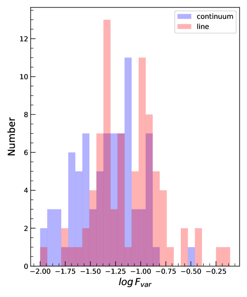
AGN have been extensively studied for their variability and it has been found that optical variability of AGN correlates with many of their physical properties. Most of these studies concentrate on photometric monitoring, however, in such studies, broad emission lines too can fall in the photometric pass band. The best way to study line and continuum variability separately is through spectroscopic monitoring observations, however, it is time consuming. A data set suitable for such a study is the one accumulated for RM studies. Though, the line and continuum light curves accumulated from RM observations and used in this work are primarily used to understand the BLR, they are also a good data set to investigate the variability of AGN. As we have both continuum and line light curves, we characterized the line and continuum variability of our sample using F_var (Edelson et al., 2002; Vaughan et al., 2003). The light curves for some objects analyzed here, were corrected for the constant host galaxy contamination to the continuum and the narrow-line contamination to the line fluxes. For few sources the host galaxy and the narrow line contribution to the continuum and line fluxes were not removed. This will have some effect on the derived F_var values reported here as the flux contribution from host galaxy could lead to low values of F_var (Peterson, 2001). However, this will not lead to biases on the comparative analysis of the F_var values between different emission lines and the continuum. The distribution of the amplitude of variability, F_var for both the continuum and line (that includes MgII, H $\beta$ and H $\alpha$ ) are given in Fig. 1. A two sample Kolmogorov-Smirnov (KS) test indicates that the two distributions are indeed different with a statistic of 0.317 and a $p$ value of 4.0 $\times$ 10^-4. We found mean F_var values of $0.057\pm 0.001$ and $0.106\pm 0.012$ for continuum and line, respectively. We have a total of 50 measurements for $\mathrm{H\beta}$ , 26 for $\mathrm{H\alpha}$ and 6 for MgII line. Separating the sample based on different lines, for $\mathrm{H\beta}$ sample, we found mean F_var values of $0.065\pm 0.002$ and $0.119\pm 0.012$ for continuum and line, respectively. For H $\alpha$ sample, the mean F_var values for continuum and line are $0.041\pm 0.001$ and $0.076\pm 0.018$ , while for MgII sample, we found mean F_var of $0.057\pm 0.001$ and $0.120\pm 0.002$ for continuum and line, respectively. The F_var in line is thus found to exceed than that of the continuum. Such increased variations in emission lines relative to the continuum support the deviation of BLR from the linear response to the ionizing continuum (Rashed et al., 2015; Li et al., 2013). Though photoionization models predict that MgII line should be less responsive to the continuum than Balmer lines (Korista & Goad, 2000, 2004), Woo (2008) found $\mathrm{F_{var}}$ in Mg II line higher than the continuum too, similar to what is found in this work. For intermediate-redshift quasars the MgII line may originate almost in the same region as $\mathrm{H\beta}$ , as can be seen in the cases of NGC 3783 and NGC 4151, for which similar time lags were obtained using $\mathrm{H\beta}$ and MgII lines (Reichert et al., 1994; Peterson et al., 2004; Metzroth et al., 2006; Woo, 2008). Therefore, it is possible to detect a similar kind of line variability in both the $\mathrm{H\beta}$ and MgII lines in these objects.

4.2 BLR characteristics

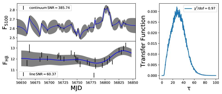
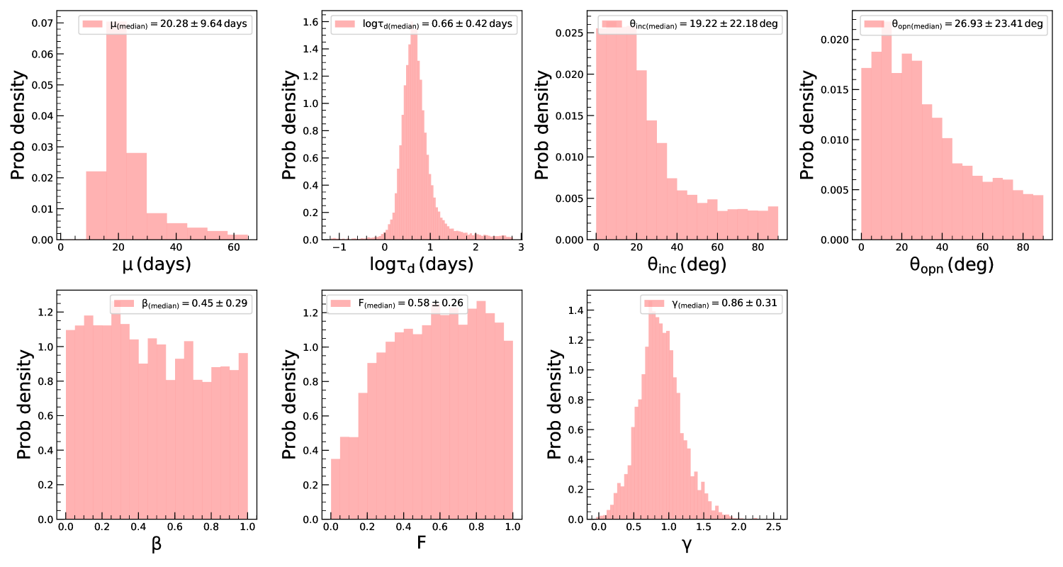
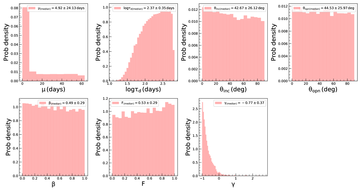
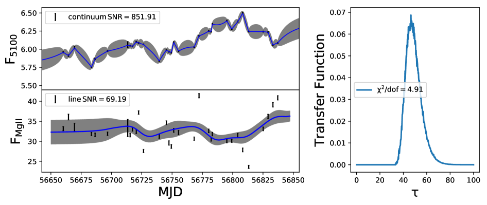
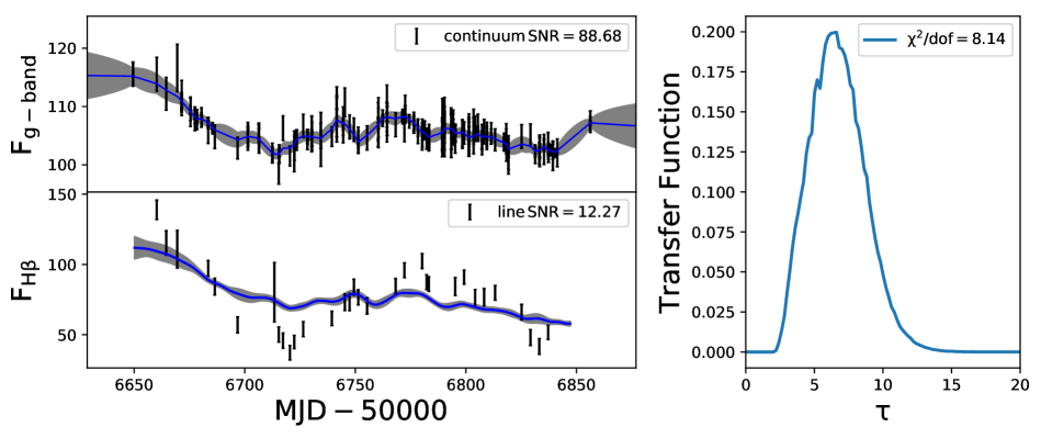
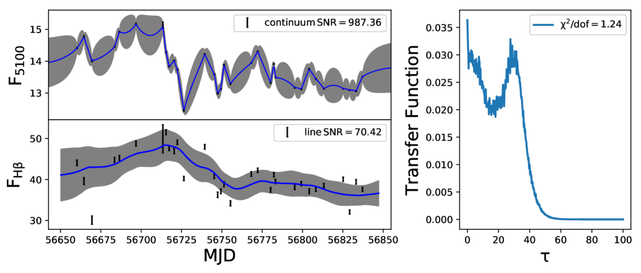
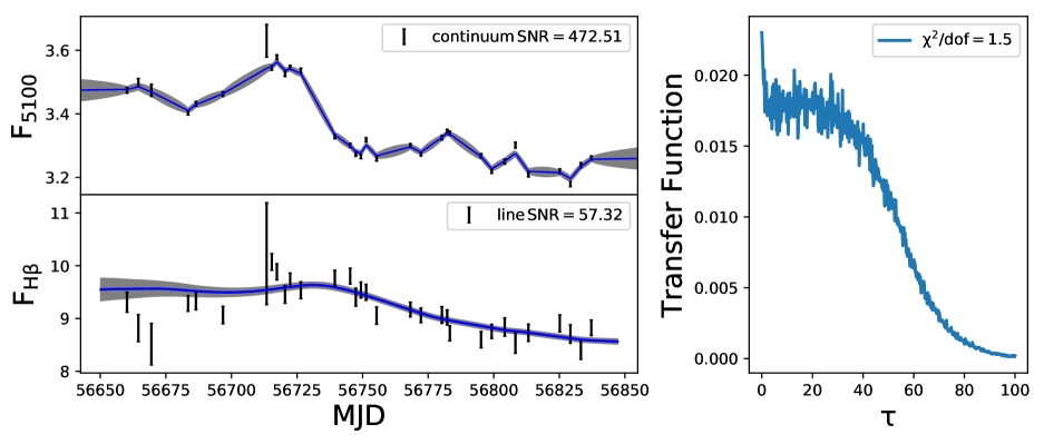
Modeling of the BLR using a Bayesian approach was developed by Pancoast et al. (2011) and subsequently applied to Arp 151 (Brewer et al., 2011) and Mrk 50 (Pancoast et al., 2012). In addition to Mrk 50 and Arp 151, more AGN were subjected to BLR modeling (Pancoast et al., 2014; Grier et al., 2017a; Williams et al., 2018; Li et al., 2013). The BLR modeling used in this work is based on Li et al. (2013), which is an independent implementation of the approach of Pancoast et al. (2011), however, with the additional inclusion of (a) non-linear response of emission lines to the continuum variations and (b) option to carry out a detrending of the light curves. Here, we analysed the data for 57 objects with 82 independent measurements for $\mathrm{H\beta}$ , $\mathrm{H\alpha}$ and MgII lines, which is twice the number of AGN studied earlier (Li et al., 2013) for uncovering the characteristics of BLR. We show in Fig. 2 few examples to illustrate our BLR model fits to their observed continuum and line reverberation data. The model reproduces the observed light curves for all the objects. In these plots the data points with error bars are the observed light curves and the thick solid lines are the reconstructed light curves by the model. For the object J1412+534, few points of the observed line light curve deviate from the reconstructed light curve. These points are also found to deviate from the general trend of the observed line light curve that results of larger $\chi^{2}/dof$ value of 4.91 pointing to poor fitting to the light curve. For the object J1421+525, there is a discrepancy between the observed and modeled line light curve. The $\chi^{2}/dof$ of 8.14 obtained here could be due to poor sampling and/or SNR of the emission line measurements. The corresponding transfer functions for those four objects are given in the right hand panel of Fig. 2. We found the transfer functions to have different shapes. For example in J1412+534 (top panel; $\alpha_{2000}$ = 14:12:14.20, $\delta_{2000}$ = 53:25:46.7), the transfer function is single peaked at $\tau$ = $\tau_{lag}$ . For this object the BLR modeling gives $\theta_{inc}$ = 4.0 $\pm$ 2.8 deg and $\theta_{opn}$ = 6.0 $\pm$ 3.9 deg. The transfer function for J1407+537 ( $\alpha_{2000}$ = 14:07:59.07, $\delta_{2000}$ = 53:47:59.8) is double peaked, for which we obtain $\theta_{inc}$ = 65.0 $\pm$ 22.1 deg and $\theta_{opn}$ = 37.0 $\pm$ 26.5 deg. For J1417+517 (bottom panel; $\alpha_{2000}$ = 14:17:06.68, $\delta_{2000}$ = 51:43:40.1), the transfer function has a top hat structure with derived $\theta_{inc}$ and $\theta_{opn}$ of 57.9 $\pm$ 21.6 deg and 51.8 $\pm$ 25.8 deg, respectively. We note that the peak of the transfer function is not always a reliable indicator for the size of the BLR. For example, peak can represent BLR size for a single peaked transfer function but it is not a reliable indicator for a double peaked transfer function or a transfer function with long tail. The first moment of transfer function, which represents the time lag in CCF analysis, gives a better estimate of the average size of the BLR (Gaskell & Sparke, 1986; Gaskell & Peterson, 1987; Kovačević et al., 2014). We found a) for a thick disk, larger $\theta_{\mathrm{inc}}$ tends to produce a double-peaked transfer function, as seen in the case of object J1407+537 (third panel of Fig. 2 from the top) with $\theta_{\mathrm{inc}}$ = 65.0 $\pm$ 22.1 deg. As $\theta_{\mathrm{inc}}$ increases, the object appears more edge on and the radiation coming both from the front and back surfaces makes a double peak transfer function where the stronger peak appears closer to the center. b) a larger opening angle $\theta_{\mathrm{opn}}$ tends to broaden the transfer functions toward top-hat as seen in case of J1417+517 (bottom panel of Fig. 2) which has a $\theta_{\mathrm{opn}}$ of 51.8 $\pm$ 25.8 degree. As $\theta_{\mathrm{opn}}$ increases the BLR tends to a spherical geometry and the virial motion of the clouds contributes to the transfer function making the transfer function broaden towards a top-hat structure.

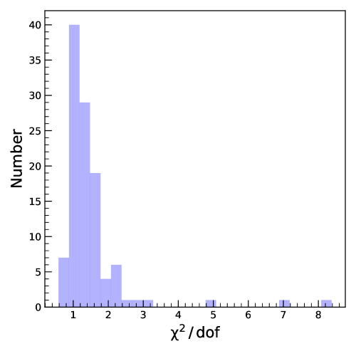
We show in Fig. 3 the distribution of $\chi^{2}/dof$ obtained for the best fit model returned by PBMAP. The fits are indeed bad (with $\chi^{2}/dof$ $>$ 4) for a few sources, namely J141214.20+532546.7, J141941.11+533649.6 and J142135.90+523138.9. These sources have poor quality (less number of points and sparsely sampled) data and is the likely cause for large $\chi^{2}$ /dof. Though the overall distribution of $\chi^{2}/dof$ seems skewed to values larger than 1.0, in majority of the sources, we obtained a low $\chi^{2}/dof$ close to 1.0. For about 60% of the light curves we obtained $\chi^{2}/dof\leq$ 1.2. The poorer $\chi^{2}/dof$ in some objects is due to them having continuum and line light curves with SNR $<$ 50. Also, systematic errors due to calibration which are usually not included in the reported uncertainties of the original data could affect the $\chi^{2}$ value. Overall, the continuum and emission line light curves generated by the model are in good agreement with the observed data.

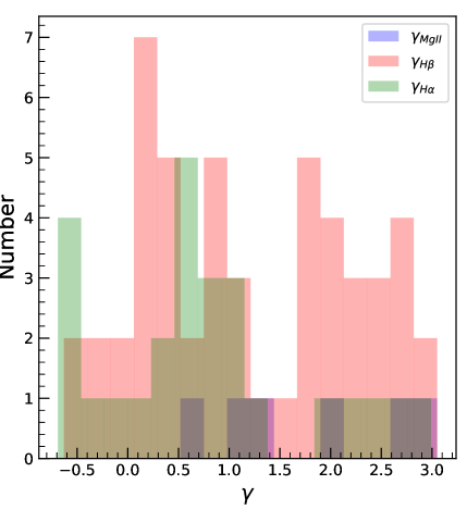
Fig. 4 shows the distribution of the non-linearity parameter $\gamma$ obtained from modeling, we found $<\gamma_{MgII}>=1.78\pm 0.86$ , $<\gamma_{H\beta}>=1.18\pm 1.03$ and $<\gamma_{H\alpha}>=0.76\pm 0.99$ for MgII, $\mathrm{H\beta}$ and $\mathrm{H\alpha}$ , respectively. This clearly indicates a non-linear response of emission-lines from BLR to the ionizing optical continuum. Such non-linear response of line flux to the ionizing continuum can be due to the anisotropic and non axis-symmetric emission coming from different spectral regions in AGN (Korista & Goad, 2000, 2004; Gaskell et al., 2019). Note that the shorter wavelength UV continuum usually vary larger compared to the longer wavelength optical continuum, therefore, depending on the continuum, the response of a given emission line could be different (O’Brien et al., 1995; Zhu et al., 2017).

4.3 Dependency of damping time scale on Luminosity at $5100\,$ Å for H ${\beta}$ line fitting

Kelly et al. (2009) modeled the light curves of 100 quasars using DRW and found the time scale of variability to correlate with luminosity. Recently, Lu et al. (2019) performed DRW modeling of 73 AGN including high-accreting sources, which are also studied here. They found that the damping time scale is strongly correlated with luminosity with a slope of $0.46\pm 0.09$ . However, MacLeod et al. (2010) using SDSS stripe 82 data, did not find any strong correlation with luminosity. In our fitting, emission line and continuum model parameters are fitted simultaneously allowing us to study this relation.

We show in Fig. 5 the dependence of the derived rest frame damping time scale on the observed host-galaxy corrected continuum luminosity at 5100 Å. We found that the damping time scale $\tau_{d}$ is positively correlated with the luminosity at 5100 Å. From linear least squares fitting to the data we found

\log\left(\frac{\tau_{d(H\beta)}}{\mathrm{1day}}\right)=\beta+\alpha\log(\lambda L_{\lambda})(5100$\r{A}$)

(9)

with $\alpha=0.54\pm 0.06$ and $\beta=-22.09\pm 2.67$ . The slope of the correlation is similar to the value of $\alpha=0.60\pm 0.06$ found by Li et al. (2013), who performed BLR modeling, in the same fashion like we did here, from an analysis of 50 AGN with H $\beta$ lags. We note that the scatter in the relation is much higher than Lu et al. (2019), mainly because they modeled continuum light curves with only two main parameters while we fitted both continuum and BLR model parameters simultaneously. Moreover, their sample does not include SDSS RM sample, which has relatively less time sampling and variability. A carefully analysis suggests that the more deviant points have lower variability and hence the model parameters are not well constrained.

To check the correlation between the damping time scale and luminosity at 5100 Å, we estimated the Spearman rank correlation coefficient ( $\mathrm{r_{s}}$ ) using Monte Carlo simulation where each point in the $\mathrm{\tau_{d}-\lambda L_{\lambda}}$ plane is modified by a random Gaussian deviate consistent with the measured uncertainty. From the distribution obtained for 10000 Monte Carlo iterations, the median value of $\mathrm{r_{s}}$ is found to be $0.218^{+0.065}_{-0.066}$ with a probability ( $p$ ) of no correlation of $0.016^{+0.079}_{-0.015}$ . The upper and lower errors are the values at the 15.9 and 84.1 percentile of the distributions of those 10000 iterations. Kozłowski (2017a, b) suggested that deriving damping time from short duration light curves leads to biased results and the time length of the light curve must be 10 times the true damping time scale. We note that reverberation light curves are usually shorter in length compared to the long-term survey light curves such as those from the Sloan Digital Sky Survey and the Catalina Real Time Transient Survey. In fact, the median ratio of the total span ( $\mathrm{\Delta t}$ ) of the light curves to the damping time scale $\tau_{d}$ is 4.84 and 4.35 for continuum and line light curves, respectively. Considering objects with light curve length $>10\times\tau_{d}$ , which includes a total 20 objects from our sample and 21 objects from Li et al. (2013), the Spearman rank correlation coefficient is found to be $0.304^{+0.104}_{-0.104}$ with $p$ -value of $0.053^{+0.155}_{-0.045}$ (10000 iterations) for the $\mathrm{\tau_{d}-\lambda L_{\lambda}}$ relation. The least-square fit using Equation 9 provides $\alpha=0.39\pm 0.08$ and $\beta=-15.99\pm 3.50$ . The correlation thus obtained between $\mathrm{\tau_{d}}$ and $\mathrm{\lambda L_{\lambda}}$ is significant at greater than 90% level. This result is consistent with Lu et al. (2019), who studied the optical variability characteristic of reverberation mapped AGN and found $\alpha=0.46\pm 0.09$ and $\beta=-18.52\pm 4.06$ in the $\mathrm{\tau_{d}-\lambda L_{\lambda}}$ relation, for sources with light curve lengths greater than 10 times $\tau_{d}$ .

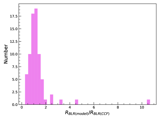
4.4 Relation between $R_{\mathrm{BLR}}^{\mathrm{mod}}$ and $R_{\mathrm{BLR}}^{\mathrm{CCF}}$

In Fig. 6 we show a comparison of the size of the BLR derived by the modeling approach ( $R_{\mathrm{BLR}}^{\mathrm{mod}}$ ) with that obtained using the conventional cross-correlation function (CCF) analysis ( $R_{\mathrm{BLR}}^{\mathrm{CCF}}$ ). The model BLR size is in general consistent with that obtained from CCF, however, with a large scatter. The median of the ratio between BLR size estimated by modeling and CCF is $1.09$ with standard deviation of $1.24$ .

Li et al. (2013) found that the BLR sizes obtained by CCF analysis are underestimated by 20 $\%$ . Although we found a few objects to have model $R_{\mathrm{BLR}}$ larger than that obtained by CCF analysis, a few others have model $R_{\mathrm{BLR}}$ smaller than that of CCF. The median of the ratio of $R_{\mathrm{BLR}}$ model to $R_{\mathrm{BLR}}$ CCF (see lower panel of Fig. 6) is found to be $1.09\pm 1.24$ , where 3 objects are found to deviate from the unit ratio by a factor larger than 3. The objects that show larger deviation from the $R_{\mathrm{BLR}}^{mod}$ = $R_{\mathrm{BLR}}^{CCF}$ line also have large $\chi^{2}/dof$ ( $>$ 1.5) values giving ample indication that the model fitting is improper which could be due to the following reasons (a) poor sampling of the light curves (b) low SNR in the light curves and (c) multiple peaks in the CCF leading to ambiguity in the determination of the peak of the CCF and subsequently $R_{\mathrm{BLR}}$ .

4.5 BLR size-luminosity relation

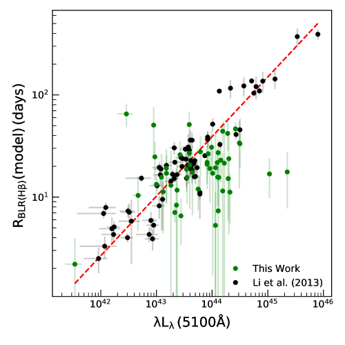
Reverberation mapping observation over the years have led to a power law relation ( $R_{\mathrm{BLR}}\propto L^{\alpha}$ ) between the size of the BLR and the optical luminosity of the AGN. The $R_{\mathrm{BLR}}-L$ relation is very important as it enables the determination of M_BH from single epoch spectroscopic observations. Also the $R_{\mathrm{BLR}}-L$ relation can provide a means to consider AGN as standard candles (Loli Martínez-Aldama et al., 2019). Therefore, it is important to check if the derived $R_{\mathrm{BLR}}$ from fitting shows the power law dependence with luminosity that we know from observation. As we have sources over a varied range of redshift, $R_{\mathrm{BLR}}$ from model fitting has been found using lines of H ${\beta}$ , H ${\alpha}$ and Mg II. The relation between $R_{\mathrm{BLR}}$ and luminosity for H ${\beta}$ is shown in Fig. 7. Note that we adopted host-corrected luminosities from the original literature ²²2 In Fig. 7, we excluded one measurement for which the host-corrected luminosity is not available in the literature. Details on host-subtraction can be found in the original literature.

Using weighted linear least squares fit we obtained the following relation

\log\left(\frac{R_{\mathrm{BLR}(H\beta)}}{\mathrm{1day}}\right)=\beta+\alpha\log(\lambda L_{\lambda})(5100$\r{A}$)

(10)

with $\alpha$ = 0.58 $\pm$ 0.03 and $\beta$ = $-$ 24.08 $\pm$ 1.13. This is similar to the value of $\alpha$ = $0.519^{+0.063}_{-0.066}$ and $\beta$ = $-21.3^{+2.9}_{-2.8}$ obtained by Bentz et al. (2009) with $R_{\mathrm{BLR}}$ obtained by CCF analysis of the observed continuum and line light curves. Bentz et al. (2013) found a slope of $\mathrm{\alpha=0.533^{+0.035}_{-0.033}}$ and $\mathrm{\beta=1.527^{+0.031}_{-0.031}}$ considering lag-luminosity relation of $\mathrm{\log\left(\frac{R_{\mathrm{BLR}(H\beta)}}{\mathrm{1day}}\right)=\beta+\alpha\log(\lambda L_{\lambda}/10^{44}\,erg\,s^{-1})}$ (5100Å). Our values closely match with those obtained by Bentz et al. (2013) considering the uncertainties. Li et al. (2013) using the approach adopted in this work for 40 quasars with $H\beta$ measurements found a value of $\alpha$ = 0.55 $\pm$ 0.03, which again is in agreement with the one found by us using a different sample of 51 AGN for the $\mathrm{H{\beta}}$ line.

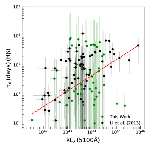
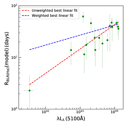
Similarly, the relation between R_BLR and $L_{5100\AA}$ for objects with $\mathrm{H\alpha}$ measurements is shown in Fig. 8. We used only measurements with fractional error less than 1. Using weighted linear least squares fit to the data we found

\log\left(\frac{R_{\mathrm{BLR}(H\alpha)}}{\mathrm{1day}}\right)=\beta+\alpha\log(\lambda L_{\lambda})(5100$\r{A}$)

(11)

with $\alpha=0.19\pm 0.12$ and $\beta=-6.86\pm 5.16$ as shown by the dashed blue line. Using unweighted linear least squares fit to the data as shown by dashed red line, we found

\log\left(\frac{R_{\mathrm{BLR}(H\alpha)}}{\mathrm{1day}}\right)=\beta+\alpha\log(\lambda L_{\lambda})(5100$\r{A}$)

(12)

with $\alpha=0.47\pm 0.08$ and $\beta=-19.10\pm 3.67$ which closely matches with $\alpha$ =0.5 based on simple photoionization arguments. We note that the unweighted fit is driven by a single data point at low luminosity. This point corresponds to the object J1342+356 (NGC 5273), which has a luminosity of $\mathrm{log\,L_{AGN}=41.534\pm 0.144}$ erg s^-1 and a BLR size of $2.06^{+1.42}_{-1.31}$ days based on $\mathrm{H\alpha}$ line obtained from traditional CCF analysis by Bentz et al. (2014). The BLR size obtained from our modeling approach is $2.29\pm 2.24$ days which is consistent with that obtained by Bentz et al. (2014).

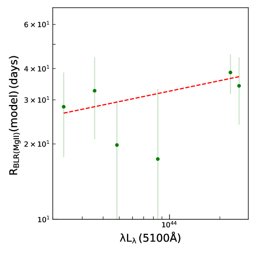
We have six objects with Mg II line light curves. For those objects the relation between R_BLR and $L_{5100\AA}$ is given in Fig. 9. We plotted the data with the form

\log\left(\frac{R_{\mathrm{BLR}(MgII)}}{\mathrm{1day}}\right)=\beta+\alpha\log(\lambda L_{\lambda})(5100$\r{A}$)

(13)

and we found $\alpha$ = $0.14\pm 0.08$ and $\beta$ = $-4.59\pm 3.58$ . The relation between $R_{\mathrm{BLR}}$ and luminosity of Mg II deviates from the value expected from photoionization argument. This is only due to the poor quality of measurement available on small number of sources. We note that the $R_{\mathrm{BLR}}-L$ relation of $\mathrm{H\alpha}$ line has a luminosity range of $10^{41.5}$ to $10^{44.1}$ $\mathrm{erg\,s^{-1}}$ and majority of them are above $10^{43}$ $\mathrm{erg\,s^{-1}}$ , whereas for Mg II line the luminosity ranges only between $10^{43.4}$ to $10^{44.4}$ $\mathrm{erg\,s^{-1}}$ . $\mathrm{R_{BLR}}$ measurements on large number of objects spanning over a wide range of luminosities are needed to firmly establish the relationship between $\mathrm{R_{BLR}}$ and luminosity based on $\mathrm{H\alpha}$ and Mg II emission lines and therefore, the coefficients of Equations 12 and 13, should be taken with caution.

4.6 The Virial factor $f_{\mathrm{BLR}}$

The virial factor $f_{\mathrm{BLR}}$ given in Equation 1 depends on factors such as the kinematics, geometry and inclination of the BLR. One of the many factors provided by the Bayesian based modeling approach carried out here is the capability to estimate $f_{\mathrm{BLR}}$ . For a disk like BLR, (see Collin et al., 2006; Li et al., 2013; Rakshit et al., 2015) $f_{\mathrm{BLR}}$ can be written as

f_{\mathrm{BLR}}\approx(\sin^{2}\theta_{\mathrm{opn}}+\sin^{2}\theta_{\mathrm{inc}})^{-1}

(14)

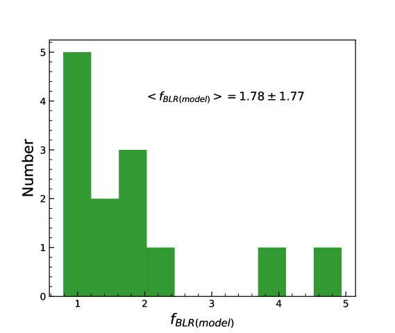
where $\theta_{\mathrm{inc}}$ is the inclination angle and $\theta_{\mathrm{opn}}$ is the opening angle of the disk. Following Li et al. (2013) we calculated $f_{\mathrm{BLR}}$ for only those objects with $\theta_{opn}$ $<$ 40^∘. Our calculated values of $f_{\mathrm{BLR}}$ range from 0.79 to 4.94, with a mean value of $1.78\pm 1.77$ . A distribution of $f_{\mathrm{BLR}}$ is shown in Fig. 10. Collin et al. (2006) found a value of $<\log(f_{\mathrm{BLR}})>$ = 0.18. Our average value of $<\log(f_{\mathrm{BLR}})>$ = 0.17 closely matches with that found by Collin et al. (2006). The large error bars in our $f_{\mathrm{BLR}}$ values are due to large uncertainties in both $\theta_{\mathrm{inc}}$ and $\theta_{\mathrm{opn}}$ .

It is also possible to get an estimate of $f_{\mathrm{BLR}}$ for sources that have stellar velocity dispersion measurements. For local inactive galaxies a tight correlation is known to exist between M_BH and bulge or spheroid stellar velocity dispersion ( $\sigma_{*}$ ). This correlation (Ferrarese & Merritt, 2000; Gebhardt et al., 2000) is given as

\log\left(\frac{M_{BH}}{M_{\odot}}\right)=\alpha+\beta\log\left(\frac{\sigma_{*}}{200\,\mathrm{kms^{-1}}}\right)

(15)

with $\alpha=8.13\pm 0.06$ and $\beta=4.02\pm 0.32$ (Tremaine et al., 2002). Assuming AGN too follow the above equation, one can estimate M_BH. Comparing this M_BH with the virial product VP = $\left(\frac{\Delta V^{2}R_{\mathrm{BLR}}}{G}\right)$ obtained by reverberation mapping, we can get an estimate of $f_{\mathrm{BLR}}$ as

f_{\mathrm{BLR}}=\frac{M_{BH}^{\sigma_{*}}}{\mathrm{VP}}.

(16)

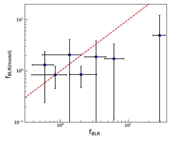
For a total of seven sources in our sample, we could obtain both the $f_{\mathrm{BLR}}$ measurements, one based on the Bayesian based BLR modeling approach and the other obtained from the ratio of $M_{\mathrm{BH}}$ based on Equation 15 to the virial product obtained from RM. We found a good correlation between the two virial factors (see Fig. 11). Considering the dispersion of $\sim 0.4$ dex in the $M_{\mathrm{BH}}-\sigma_{*}$ relation our 1D modeling approach is able to provide $f_{\mathrm{BLR}}$ consistent with that obtained from RM method and M_BH and $\sigma_{*}$ relation. From linear least squares fit to the data points in Fig. 11, we found a Spearman rank correlation coefficient of $0.29^{+0.39}_{-0.54}$ and a p-value of $0.38^{+0.44}_{-0.31}$ . Removing the data point with $\mathrm{f_{BLR}}$ $>$ 10, also the one with very large uncertainty, linear least squares fit gave a linear correlation coefficient of 0.14 ${}^{+0.46}_{-0.51}$ and a $p$ value of $0.47^{+0.40}_{-0.31}$ . Though, the points are scattered around the dotted line in Fig. 11, the derived $\mathrm{f_{BLR(model)}}$ have large error bars and this could be the reason for no tight correlation between the scale factors obtained by both the methods. Most of the values of $\mathrm{f_{BLR(model)}}$ are found to be lesser than 3, which points to a BLR with a thick geometry and viewed at an inclination angle. Given the fact that $f_{\mathrm{BLR}}$ has a large range, the M_BH values obtained from single epoch measurements adopting a single $f_{\mathrm{BLR}}$ are bound to have large uncertainties. Mejía-Restrepo et al. (2018) by comparing $M_{\mathrm{BH}}$ obtained by accretion disk model fitting and virial methods found that $f_{\mathrm{BLR}}$ is correlated with the width of the broad emission lines as $f_{\mathrm{BLR}}\propto\mathrm{FWHM}^{-1}$ .

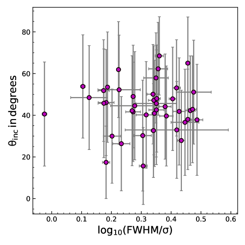
Also, the ratio of FWHM to the line dispersion of broad H ${\beta}$ line is suggested to be correlated with the inclination angle (Collin et al., 2006; Goad et al., 2012). However, Pancoast et al. (2014) could not find any correlation using a small sample of 5 objects having good quality measurements. We used the available FWHM and line dispersion measurements from the RMS spectra of broad $\mathrm{H\beta}$ line collected from the literature. We plot the inclination angle from the model as a function of the ratio of the FWHM to the line dispersion in Fig. 12. We do not find any strong correlation. Though our measurements have large error bars, the results agree with the finding of Pancoast et al. (2014).

4.7 Measurement of $M_{BH}$ and accretion rates

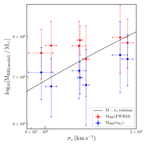
Black hole masses are calculated using Equation 1, where we adopted $f_{\mathrm{BLR}}$ and $R_{\mathrm{BLR}}$ of the $\mathrm{H\beta}$ line obtained from the model. The velocity width $\Delta V$ can be measured either from the full width at half maximum (FWHM) or from the line dispersion $\sigma_{\mathrm{H\beta}}$ . We estimated the black hole masses for those 11 objects which have $f_{\mathrm{BLR}}(\mathrm{model})$ measurements using both FWHM and line dispersion $\sigma_{\mathrm{H\beta}}$ separately as $\sigma_{\mathrm{H\beta}}$ gives less biased $\mathrm{M_{BH}}$ measurement than using the FWHM (Peterson, 2011; Grier et al., 2012). In Fig. 13, we compared the $\mathrm{M_{BH(model)}}$ values with the $\mathrm{M-\sigma_{*}}$ relation as given in Equation 15. We found that most of the $\mathrm{M_{BH(model)}}$ measurements using FWHM lie above $\mathrm{M-\sigma_{*}}$ relation, whereas, most of the $\mathrm{M_{BH(model)}}$ values obtained using $\sigma_{\mathrm{H\beta}}$ lie below the $\mathrm{M-\sigma_{*}}$ line. But considering the uncertainties all $\mathrm{M_{BH(model)}}$ measurements are found to be consistent with the $\mathrm{M-\sigma_{*}}$ relation.

We also calculated the dimensionless accretion rate as given by Du et al. (2018)

\dot{M}=20.1\left(\frac{L_{44}}{\cos i}\right)^{3/2}m_{7}^{-2}

(17)

where $m_{7}=M_{\mathrm{BH}}/10^{7}M_{\odot}$ , $L_{44}=L_{5100}/10^{44}ergs^{-1}$ and $i$ is the inclination angle. Our obtained values for those 11 objects as mentioned in Table 8 indicate low to moderately accreting black holes with $\dot{M}$ ranging from 0.002 to 2.266.

Table 8:

M_{\mathrm{BH}}

and accretion rate

\dot{M}

measurements.

$\alpha_{2000}$	$\delta_{2000}$	$\log(M_{\mathrm{BH}})(\mathrm{FWHM})$	$\log(M_{\mathrm{BH}})(\sigma_{\mathrm{H\beta}})$	$\dot{M}$
02:30:05.52	-08:59:53.2	$7.98\pm 0.70$	$7.53\pm 0.70$	0.018
06:52:12.32	+74:25:37.2	$8.51\pm 0.85$	$7.67\pm 0.54$	0.011
14:07:59.07	+53:47:59.8	$7.91\pm 0.38$	$6.99\pm 0.37$	0.232
14:10:31.33	+52:15:33.8	$7.84\pm 0.63$	$7.43\pm 0.62$	0.510
14:11:12.72	+53:45:07.1	$7.58\pm 0.62$	$7.11\pm 0.61$	2.266
14:13:18.96	+54:32:02.4	$7.76\pm 0.66$	$7.15\pm 0.63$	0.563
14:16:25.71	+53:54:38.5	$7.75\pm 0.35$	$7.03\pm 0.33$	2.188
14:20:39.80	+52:03:59.7	$8.14\pm 0.60$	$7.27\pm 0.60$	0.187
14:20:49.28	+52:10:53.3	$9.29\pm 0.59$	$8.93\pm 0.58$	0.002
14:21:03.53	+51:58:19.5	$7.77\pm 0.65$	$6.79\pm 0.65$	0.211
14:21:35.90	+52:31:38.9	$7.43\pm 0.86$	$6.82\pm 0.85$	0.420

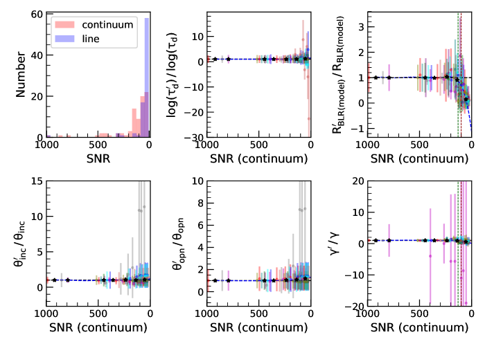
4.8 Reliability of the recovered model parameters: effect of signal to noise ratio

Modeling of the continuum and line light curves to estimate various BLR parameters depends on the SNR of the light curves. Collier et al. (2001) and Horne et al. (2004) suggested that BLR parameters can be well recovered (a) with continuum light curves of SNR $\sim$ 100 and (b) line light curves of SNR $\sim$ 30. But it is often difficult to find RM data satisfying the above mentioned qualities.

The distribution of the SNR of the continuum and line light curves used in this work is shown in Fig. 14 (top left). They span a wide range from as low as 5 to as high as 1000. The median SNR of the continuum and line light curves used in this work is about 84 and 30, respectively. To access the effects of SNR on the derived BLR parameters, we carried out simulations. We firstly selected objects with continuum light curves with SNR greater than 300. We arrived at a total of 10 objects. We then degraded the SNR of the continuum and line light curves of those 10 objects by multiplying a factor of 2, 3, 4, 5, 8, 10 and 15 to the original flux errors and adding a Gaussian random deviate of zero mean and standard deviation given by the new flux errors. We then applied the PBMAP code on the simulated light curves and extracted the BLR parameters. Here, the ratio of the recovered to the original BLR parameters are plotted against the continuum SNR. It is evident from Fig. 14, that this ratio is close to unity for most of the BLR parameters, except for the radius of the BLR, where it is found to deviate by 10% and 30%, when the SNR of the continuum are 130 and 100, as shown by the vertical green and red lines, respectively. Similarly, for the line light curves too, we found that the ratio of the recovered to the original BLR parameters are close to unity except for the BLR size, which deviates by 10% and 30%, when the SNR of the line are 25 and 15, respectively. This is also in agreement with the continuum SNR cut-off of 100 suggested by Collier et al. (2001) and Horne et al. (2004) to extract BLR parameters from RM data and line SNR cut-off of 15, considering an accuracy of 70% to the original recovered parameters.

For the 57 objects studied in this work, we have a total of 82 different measurements of $\mathrm{H\beta}$ , $\mathrm{H\alpha}$ and MgII lines, out of which $\sim 42$ % of objects have continuum and line SNR greater than 100 and 15, respectively. Also, for all the objects the BLR sizes obtained from model fits are consistent with those obtained from conventional CCF analysis within the errors. However, as the SNR is found to have a major effect on the derived sizes of the BLR from the simulations, we note that the values of the size of the BLR obtained for sources with continuum and line light curves with SNR lesser than 100 and 15, respectively, needs to be used with caution. We also carried out an analysis of the correlation of $\tau_{d}$ and the BLR sizes obtained from model to the luminosity to only those sources that have the continuum and line light curves SNR greater than 100 and 15, respectively. Though the trend of the correlation is similar to that of the full sample, the significance of the correlation is not strong due to the low number of sources.

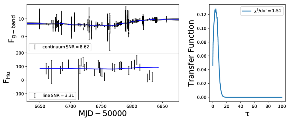
We show in Appendix B (see Fig. 16), sample light curves and the recovered transfer functions for two sources. One belongs to J1411+537 that has good quality light curves with continuum and line SNR of about 386 and 60, respectively. The other light curves belong to J1417+519, that has SNR of about 9 and 3 for the continuum and line light curves, respectively. From these light curves it is clear that BLR parameters are well constrained only for sources with good SNR data.

5 Summary

We analysed RM data collected from the literature for a total of 57 AGN that includes 51 AGN with $\mathrm{H\beta}$ data, 26 AGN with $\mathrm{H\alpha}$ data and 6 AGN with MgII line data. The main motivation is to constrain the structure and dynamics of the BLR that emits MgII, $\mathrm{H\beta}$ and $\mathrm{H\alpha}$ . We summarize our results below

1.

The estimated BLR sizes using our approach are in general consistent with that calculated from conventional CCF analysis.
2.

The best-fitted model $\mathrm{H\beta}$ BLR size is correlated with $L_{5100{\AA}}$ having a slope of $0.58\pm 0.03$ . This is similar to what is known in literature from CCF analysis. We also examined the correlation of R_BLR (H $\alpha$ ) with the continuum luminosity at 5100 Å and found a slope of $0.47\pm 0.08$ similar to what is expected from photo-ionization calculations. However more $\mathrm{H\alpha}$ measurements are needed to better constrain this correlation.
3.

We estimated virial factor using geometrical parameters and obtained a mean of 1.78 $\pm$ 1.77. The model virial factor is consistent with the virial factor obtained by the ratio of M_BH from $M-\sigma_{*}$ relation to the virial product (VP) obtained from RM. Using line light curves only it is not possible to constrain the virial factor $f_{BLR}$ (Li et al., 2013). For that reason our measured $f_{BLR}$ have large uncertainties because of large errors present in both $\theta_{inc}$ and $\theta_{opn}$ obtained from the model fitting.
4.

We found a close correspondence between the BLR size found from model and that estimated from CCF analysis, however, some objects do show large deviation. The objects that show large deviation from the R ${}_{\mathrm{BLR}}(\mathrm{model})$ = R ${}_{\mathrm{BLR}}(\mathrm{CCF})$ line have poor quality light curves.
5.

The mean value of the non linearity parameter $\gamma$ is found to be non zero for different lines indicating deviation from linear response of the line emission to the optical ionizing continuum. This may be due to a) the anomalous behaviour of the BLR region because of the poor correlation between optical continuum variability and the ionizing continuum variability (Edelson et al., 1996; Maoz et al., 2002; Gaskell et al., 2019) and b) anisotropic line emission from the partially optically thick BLR. This anisotropic effect is not considered in the model used here.
6.

Variability analysis of the sample indicates that line varies more than the continuum. The damping time scale obtained from modeling is found to be positively correlated with the continuum luminosity at 5100 Å.
7.

From the analysis of the simulated light curves, we conclude that reliable estimation of BLR size as well as other parameters via the modeling approach requires continuum and line light curves with SNR greater than 100 and 15, respectively.

This work has considerably increased the number of objects investigated through geometrical modeling of the BLR. Despite that, we were able to estimate $f_{\mathrm{BLR}}$ for only about a dozen objects. Analysis of high quality data sets for more number of AGN are needed to find precise estimates of $f_{\mathrm{BLR}}$ which can then be used with the conventional RM techniques to estimate more accurate M_BH values.

Acknowledgements

We thank the referee for valuable comments and suggestions that helped to improve the quality of the manuscript. We are thankful to Yan-Rong Li (IHEP, CAS) for making the code PBMAP available and providing instruction to run the code. AKM and RS acknowledge support from the National Academy of Sciences, India.

Data availability

The data used in this article are taken from the literature, the references of which are given in Table 1.

References

Antonucci (1993) Antonucci R., 1993, ARA&A, 31, 473
Barvainis (1987) Barvainis R., 1987, ApJ, 320, 537
Bentz & Katz (2015) Bentz M. C., Katz S., 2015, PASP, 127, 67
Bentz et al. (2009) Bentz M. C., Peterson B. M., Netzer H., Pogge R. W., Vestergaard M., 2009, ApJ, 697, 160
Bentz et al. (2010) Bentz M. C., et al., 2010, ApJ, 720, L46
Bentz et al. (2013) Bentz M. C., et al., 2013, ApJ, 767, 149
Bentz et al. (2014) Bentz M. C., et al., 2014, ApJ, 796, 8
Blandford & McKee (1982) Blandford R. D., McKee C. F., 1982, ApJ, 255, 419
Brewer et al. (2011) Brewer B. J., et al., 2011, ApJ, 733, L33
Carilli et al. (2019) Carilli C. L., Perley R. A., Dhawan V., Perley D. A., 2019, ApJ, 874, L32
Collier et al. (2001) Collier S., Peterson B. M., Horne K., 2001, in Peterson B. M., Pogge R. W., Polidan R. S., eds, Astronomical Society of the Pacific Conference Series Vol. 224, Probing the Physics of Active Galactic Nuclei. p. 457
Collin et al. (2006) Collin S., Kawaguchi T., Peterson B. M., Vestergaard M., 2006, A&A, 456, 75
Denney et al. (2010) Denney K. D., et al., 2010, ApJ, 721, 715
Du et al. (2014) Du P., et al., 2014, ApJ, 782, 45
Du et al. (2016) Du P., et al., 2016, ApJ, 825, 126
Du et al. (2018) Du P., et al., 2018, ApJ, 856, 6
Edelson & Krolik (1988) Edelson R. A., Krolik J. H., 1988, ApJ, 333, 646
Edelson et al. (1996) Edelson R. A., et al., 1996, ApJ, 470, 364
Edelson et al. (2002) Edelson R., Turner T. J., Pounds K., Vaughan S., Markowitz A., Marshall H., Dobbie P., Warwick R., 2002, ApJ, 568, 610
Ferrarese & Merritt (2000) Ferrarese L., Merritt D., 2000, ApJ, 539, L9
GRAVITY Collaboration et al. (2019) GRAVITY Collaboration et al., 2019, arXiv e-prints, p. arXiv:1910.00593
Gaskell & Peterson (1987) Gaskell C. M., Peterson B. M., 1987, ApJS, 65, 1
Gaskell & Sparke (1986) Gaskell C. M., Sparke L. S., 1986, ApJ, 305, 175
Gaskell et al. (2019) Gaskell C. M., Bartel K., Deffner J. N., Xia I., 2019, arXiv e-prints, p. arXiv:1909.06275
Gebhardt et al. (2000) Gebhardt K., et al., 2000, ApJ, 539, L13
Goad et al. (2012) Goad M. R., Korista K. T., Ruff A. J., 2012, MNRAS, 426, 3086
Gravity Collaboration et al. (2018) Gravity Collaboration et al., 2018, Nature, 563, 657
Grier et al. (2012) Grier C. J., et al., 2012, ApJ, 755, 60
Grier et al. (2013) Grier C. J., et al., 2013, ApJ, 764, 47
Grier et al. (2017a) Grier C. J., Pancoast A., Barth A. J., Fausnaugh M. M., Brewer B. J., Treu T., Peterson B. M., 2017a, ApJ, 849, 146
Grier et al. (2017b) Grier C. J., et al., 2017b, ApJ, 851, 21
Ho & Kim (2014) Ho L. C., Kim M., 2014, ApJ, 789, 17
Horne et al. (2004) Horne K., Peterson B. M., Collier S. J., Netzer H., 2004, PASP, 116, 465
Kelly et al. (2009) Kelly B. C., Bechtold J., Siemiginowska A., 2009, ApJ, 698, 895
Korista & Goad (2000) Korista K. T., Goad M. R., 2000, ApJ, 536, 284
Korista & Goad (2004) Korista K. T., Goad M. R., 2004, ApJ, 606, 749
Koshida et al. (2014) Koshida S., et al., 2014, ApJ, 788, 159
Kovačević et al. (2014) Kovačević A., Popović L. Č., Shapovalova A. I., Ilić D., Burenkov A. N., Chavushyan V. H., 2014, Advances in Space Research, 54, 1414
Kozłowski (2017a) Kozłowski S., 2017a, A&A, 597, A128
Kozłowski (2017b) Kozłowski S., 2017b, ApJ, 835, 250
Kozłowski et al. (2010) Kozłowski S., et al., 2010, ApJ, 708, 927
Landt et al. (2019) Landt H., et al., 2019, arXiv e-prints, p. arXiv:1908.01627
Li et al. (2013) Li Y.-R., Wang J.-M., Ho L. C., Du P., Bai J.-M., 2013, ApJ, 779, 110
Li et al. (2018) Li Y.-R., et al., 2018, ApJ, 869, 137
Li et al. (2019) Li Y.-R., Zhang Z.-X., Jin C., Du P., Cui L., Liu X., Wang J.-M., 2019, arXiv e-prints, p. arXiv:1909.04511
Loli Martínez-Aldama et al. (2019) Loli Martínez-Aldama M., Czerny B., Kawka D., Karas V., Zajaček M., Życki P. T., 2019, arXiv e-prints, p. arXiv:1903.09687
Lu et al. (2019) Lu K.-X., et al., 2019, ApJ, 877, 23
Lynden-Bell (1969) Lynden-Bell D., 1969, Nature, 223, 690
MacLeod et al. (2010) MacLeod C. L., et al., 2010, ApJ, 721, 1014
Mandal et al. (2018) Mandal A. K., et al., 2018, MNRAS, 475, 5330
Mandal et al. (2020) Mandal A. K., et al., 2020, MNRAS,
Maoz et al. (2002) Maoz D., Markowitz A., Edelson R., Nand ra K., 2002, AJ, 124, 1988
Mejía-Restrepo et al. (2018) Mejía-Restrepo J. E., Lira P., Netzer H., Trakhtenbrot B., Capellupo D. M., 2018, Nature Astronomy, 2, 63
Metzroth et al. (2006) Metzroth K. G., Onken C. A., Peterson B. M., 2006, ApJ, 647, 901
O’Brien et al. (1995) O’Brien P. T., Goad M. R., Gondhalekar P. M., 1995, MNRAS, 275, 1125
Onken et al. (2004) Onken C. A., Ferrarese L., Merritt D., Peterson B. M., Pogge R. W., Vestergaard M., Wandel A., 2004, ApJ, 615, 645
Pancoast et al. (2011) Pancoast A., Brewer B. J., Treu T., 2011, ApJ, 730, 139
Pancoast et al. (2012) Pancoast A., et al., 2012, ApJ, 754, 49
Pancoast et al. (2014) Pancoast A., Brewer B. J., Treu T., Park D., Barth A. J., Bentz M. C., Woo J.-H., 2014, MNRAS, 445, 3073
Peterson (1993) Peterson B. M., 1993, PASP, 105, 247
Peterson (2001) Peterson B. M., 2001, in Aretxaga I., Kunth D., Mújica R., eds, Advanced Lectures on the Starburst-AGN. p. 3 (arXiv:astro-ph/0109495), doi:10.1142/9789812811318_0002
Peterson (2011) Peterson B. M., 2011, arXiv e-prints, p. arXiv:1109.4181
Peterson et al. (1998) Peterson B. M., Wanders I., Horne K., Collier S., Alexander T., Kaspi S., Maoz D., 1998, PASP, 110, 660
Peterson et al. (2004) Peterson B. M., et al., 2004, ApJ, 613, 682
Peterson et al. (2014) Peterson B. M., et al., 2014, ApJ, 795, 149
Pozo Nuñez et al. (2014) Pozo Nuñez F., et al., 2014, A&A, 561, L8
Rafter et al. (2013) Rafter S. E., Kaspi S., Chelouche D., Sabach E., Karl D., Behar E., 2013, ApJ, 773, 24
Rakshit et al. (2015) Rakshit S., Petrov R. G., Meilland A., Hönig S. F., 2015, MNRAS, 447, 2420
Rani et al. (2017) Rani P., Stalin C. S., Rakshit S., 2017, MNRAS, 466, 3309
Rashed et al. (2015) Rashed Y. E., Eckart A., Valencia-S. M., García-Marín M., Busch G., Zuther J., Horrobin M., Zhou H., 2015, MNRAS, 454, 2918
Reichert et al. (1994) Reichert G. A., et al., 1994, ApJ, 425, 582
Salpeter (1964) Salpeter E. E., 1964, ApJ, 140, 796
Shapovalova et al. (2013) Shapovalova A. I., et al., 2013, A&A, 559, A10
Shen et al. (2016) Shen Y., et al., 2016, ApJ, 818, 30
Suganuma et al. (2006) Suganuma M., et al., 2006, ApJ, 639, 46
Tremaine et al. (2002) Tremaine S., et al., 2002, ApJ, 574, 740
Ulrich & Horne (1996) Ulrich M.-H., Horne K., 1996, MNRAS, 283, 748
Ulrich et al. (1997) Ulrich M.-H., Maraschi L., Urry C. M., 1997, ARA&A, 35, 445
Urry & Padovani (1995) Urry C. M., Padovani P., 1995, PASP, 107, 803
Vaughan et al. (2003) Vaughan S., Edelson R., Warwick R. S., Uttley P., 2003, MNRAS, 345, 1271
Wagner & Witzel (1995) Wagner S. J., Witzel A., 1995, ARA&A, 33, 163
Wandel et al. (1999) Wandel A., Peterson B. M., Malkan M. A., 1999, ApJ, 526, 579
Wang et al. (2014) Wang J.-M., et al., 2014, ApJ, 793, 108
Welsh (1999) Welsh W. F., 1999, PASP, 111, 1347
Williams et al. (2018) Williams P. R., et al., 2018, ApJ, 866, 75
Woo (2008) Woo J.-H., 2008, AJ, 135, 1849
Woo et al. (2015) Woo J.-H., Yoon Y., Park S., Park D., Kim S. C., 2015, ApJ, 801, 38
Xiao et al. (2018) Xiao M., et al., 2018, ApJ, 864, 109
Zhu et al. (2017) Zhu D., Sun M., Wang T., 2017, The Astrophysical Journal, 843, 30
Zu et al. (2011) Zu Y., Kochanek C. S., Peterson B. M., 2011, ApJ, 735, 80

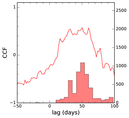
Appendix A BLR lag measurement of J1420+526 for $\mathrm{H\alpha}$ line using ICCF

Grier et al. (2017b) did not perform CCF analysis to measure the H $\alpha$ lag for the object J1420+526. We estimated the H $\alpha$ lag for this object using Interpolated Cross-correlation Function (ICCF) analysis method as shown in Fig. 15. The lag and its uncertainty are estimated using a Monte Carlo simulation based on the flux randomization (FR) and random subset selection (RSS) described in Peterson et al. (1998), Wandel et al. (1999) and Peterson et al. (2004). The median of the centroid distribution is considered as final lag while uncertainties were estimated within a 68 $\%$ confidence interval around the median value. We obtained the rest frame H $\alpha$ lag of $32.22^{+7.75}_{-11.55}$ days from ICCF method. The lag estimated based on modeling is $46.67\pm 9.8$ days which is consistent with CCF lag within error bars.

Appendix B Examples of model fit light curves and transfer functions

We show in Figure 16 light curves for two objects, namely J1411+537 having high SNR in the continuum and line, and J1411+537 having poor SNR in both the light curves. From the figure it is evident that the geometrical model parameters ( $\theta_{\mathrm{inc}}$ and $\theta_{\mathrm{opn}}$ ) are well-constrained for J1411+537 but not constrained for J1411+537. This is due to the low SNR of the continuum and line light curves in J1411+537.