Euclid. I. Overview of the Euclid mission††thanks: Dedicated to our friends and colleagues Olivier Le Fèvre (1960–2020) and Nick Kaiser (1954–2023), who contributed so much to the Euclid mission and its underlying science.
The current standard model of cosmology successfully describes a variety of measurements, but the nature of its main ingredients, dark matter and dark energy, remains unknown. Euclid is a medium-class mission in the Cosmic Vision 2015–2025 programme of the European Space Agency (ESA) that will provide high-resolution optical imaging, as well as near-infrared imaging and spectroscopy, over about 14 000 deg2 of extragalactic sky. In addition to accurate weak lensing and clustering measurements that probe structure formation over half of the age of the Universe, its primary probes for cosmology, these exquisite data will enable a wide range of science. This paper provides a high-level overview of the mission, summarising the survey characteristics, the various data-processing steps, and data products. We also highlight the main science objectives and expected performance.
Key Words.:
Cosmology: observations – space vehicles: instruments – instrumentation: detectors – surveys – Techniques: imaging spectroscopy – Techniques: photometric1 Introduction
A century of ever improving observations has resulted in a concordance cosmological model that is surprisingly simple: only six numbers are currently needed to describe a wide variety of precise measurements (Planck Collaboration VI 2020). The result, however, is also unsatisfactory because it highlights a serious problem for our understanding of fundamental physics and astronomy: it relies on assumptions about the initial conditions and the theory of gravity, while the nature of the main ingredients, dark matter and dark energy, remain great mysteries. The observational evidence for a largely ‘dark’ universe is overwhelming, demonstrating that our theories of particle physics and/or gravity are either incomplete or incorrect. Moreover, we lack compelling theoretical guidance to solve this crisis in fundamental physics (Albrecht et al. 2006; Amendola et al. 2018).
Arguably, the biggest challenge is the observation that the expansion of the Universe is accelerating (e.g. Riess et al. 1998; Perlmutter et al. 1999; Eisenstein et al. 2005; Betoule et al. 2014). Current explanations range from Einsteins cosmological constant, dynamic mechanisms such as quintessence, or a modification of the laws of gravity on cosmological scales (see Amendola et al. 2018, for an extensive overview of ideas). To robustly distinguish between these different theoretical ideas, the precision of the measurements needs to improve by at least an order of magnitude, whilst our ability to interpret the data correctly has to advance accordingly if we are to take advantage of the smaller statistical uncertainties.
The exquisite observations of the temperature fluctuations in the cosmic microwave background (CMB) performed by WMAP (Hinshaw et al. 2013) and Planck (Planck Collaboration I 2020) have been crucial to establish the baseline cosmological constant-dominated cold dark matter (CDM) model. This is because the physical interpretation of the measurements is relatively straightforward, and all-sky experiments from space benefit from a stable environment and superior control of instrumental effects. Unfortunately, the CMB provides limited information about the nature of dark matter and dark energy, because it primarily probes the physical conditions at the time of recombination, when dark energy was negligible. To quantify how the balance between dark matter and dark energy evolved, the CMB results need to be complemented by high-quality measurements of the cosmic expansion history and the growth of large-scale structure (LSS) over the past eight billion years or more. In principle, such studies can provide complementary constraints on the initial conditions, explore modifications of the theory of general relativity on cosmological scales, and determine the neutrino mass scale (Albrecht et al. 2006). Research in observational cosmology is therefore shifting towards studies of the LSS, and a number of large spectroscopic and imaging surveys will collect vast amounts of data in the coming decade. For instance, the Legacy Survey of Space and Time (LSST) by the Vera C. Rubin Observatory will repeatedly image the entire southern sky in multiple bands (Ivezić et al. 2019), while the Dark Energy Spectroscopic Instrument experiment (DESI) will measure redshifts for about 40 million galaxies (DESI Collaboration et al. 2024). These projects are major improvements over previous surveys, but a robust interpretation is essential. Accounting for the complexities of ground-based data, in particular the variable sky conditions, presents a major challenge. Hence, further advances will come from space-based facilities, such as Euclid (Laureijs et al. 2011) and the planned Nancy Grace Roman Space Telescope (Akeson et al. 2019).
This paper describes the background, instruments, performance, and planned science of Euclid, a medium-class mission in the Cosmic Vision 2015–2025 programme of the European Space Agency (ESA). Euclid resulted from a 2007 call by ESA for the selection of a medium-sized space mission. Besides five other mission proposals, a dark energy mission concept was included for competitive down-selection. This new mission concept, ultimately named Euclid, was based on a combination of two initial dark-energy mission proposals, the Dark Universe Explorer (DUNE; Refregier 2009) and the Spectroscopic All-Sky Cosmic Explorer (SPACE; Cimatti et al. 2009). It envisioned an extragalactic sky survey with visual imaging, and near-infrared photometry and spectroscopy, optimised for the measurement of the two primary cosmology probes, namely galaxy clustering and weak gravitational lensing, which are both powerful ways of measuring the evolution of the LSS, whilst complementing each other in terms of constraining power.
The main science case of Euclid was presented in Laureijs et al. (2011), which formed the basis for the official selection of the concept by ESA in 2011, and adoption as a mission in 2012. Since then, the mission hardware and software have been built, culminating in the successful launch of Euclid on 1st July 2023 on a Falcon-9 rocket from Cape Canaveral. Here we provide an up-to-date high-level overview of the mission during its initial time in orbit, describing the survey, the data products, and the science that the Euclid Consortium aims to perform.
The structure of this paper is as follows. In Sect. 2 we summarise the main science objectives of the Euclid mission and introduce the primary cosmological probes that drove the design. In Sect. 3 we provide a brief overview of the spacecraft and its instruments. The survey characteristics and supporting observations are described in Sect. 4, while early results from the commissioning and performance verification are presented in Sect. 5. The main data products that will be released publicly comprise simulated data (Sect. 6) and the actual data processed through the Euclid Science Ground Segment (SGS) pipeline (Sect. 7). The cosmological inferences enabled by Euclid are discussed in Sect. 8. Additional cosmological probes that are enabled or enhanced by the Euclid data are reviewed in Sect. 9. Finally, the impact of Euclid is not limited to cosmology, and a taste of the wide range of astrophysics that will be done is presented in more detail in Sect. 10. To aid in the readability of this and accompanying papers, we include a glossary of acronyms in Appendix A. Unless specified otherwise, magnitudes and surface brightness values are reported using the AB magnitude system.
2 Primary probes for cosmology with Euclid
The biggest mysteries in cosmology are the nature of dark matter and dark energy. Indirect evidence for the existence of dark matter has come from a wide range of astronomical and cosmological observations, but if it is composed of new elementary particles outside the standard model of particle physics, direct detections in terrestrial experiments (e.g. Battaglieri et al. 2017) are likely to play a prominent role in establishing its nature. The situation is markedly different for the observed accelerating expansion of the Universe, where progress will most likely come from advances in observational cosmology. To explain the observations, a component with a negative equation-of-state parameter111The equation-of-state parameter relates the pressure and the energy density of a substance as . In the case of a cosmological constant , or a non-zero vacuum energy density, , and the time derivative is zero. is required, which is commonly referred to as dark energy. It makes up about 69% of the present-day energy density (Planck Collaboration VI 2020), but we do not know if it is a cosmological constant, a field that evolves dynamically, or reflects a more profound modification of the gravitation laws at cosmological scales (see e.g. Amendola et al. 2018). One of the key observables to distinguish between such models is the way the equation-of-state parameter varies with redshift. To allow for a convenient comparison between cosmological probes, we adopt
| (1) |
which captures the dynamical nature of dark energy to first order in , where is the scale factor. Here, is the present day equation of state, and quantifies the dependence with redshift. This extension corresponds to a basic non-clustering dynamical dark energy model, and constraints on the parameters and show how well Euclid can test this scenario. For completeness, we note that the cosmological constant corresponds to the choice and .
We can quantify the performance of a particular survey by comparing the dark energy figure of merit (FoM), which we defined as the inverse square root of the covariance matrix determinant for the dark energy parameters (Wang 2008b),
| (2) |
so that a larger value implies a more precise measurement of the dark energy properties.222To evaluate the FoM we marginalise over the cosmological and nuisance parameters, while imposing a Gaussian prior on the baryon density from big bang nucleosynthesis (BBN). See Sect. 8.2.3 for more details. The challenge for the experimental design, however, is to establish a minimum value to achieve. Laureijs et al. (2011) presented a statistical argument, concluding that the value of needs to be determined with a precision of about 1% to robustly test the CDM model. Specifically, one of the main objectives of Euclid is to constrain the dark energy equation of state so that for this baseline scenario.
This is a challenging target for two reasons. First, to achieve such statistical constraining power requires surveying a considerable fraction of the cosmological volume out to (see e.g. Amara & Réfrégier 2007), thus covering the epoch during which dark energy became the dominant component in the Universe. In the case of Euclid, the aim is to observe 14 000 deg2 of extragalactic sky with low zodiacal background and low Galactic extinction (see Sect. 4 for details). Second, systematic biases need to be sufficiently small as to not overwhelm the orders of magnitude improvement in precision. The observational signatures of dark energy are subtle, and unrecognised instrumental effects could be mistaken for new physics. To minimise this, exquisite experimental control is paramount. Although still challenging (and dependent on the specific probe used), this is best achieved from space.
A measurement of the expansion history via the distance-redshift relation provides the most direct constraints on the equation of state of dark energy. More generally, it provides constraints on the relative balance of ingredients and spatial curvature via the Friedmann equations, which link the time evolution of the scale factor to these ingredients. The rate at which density fluctuations grow also depends on the background cosmology. Hence, studying the growth of LSS provides another way to infer information about the composition of the Universe. It has the added benefit that it can constrain additional cosmological parameters and provide some key tests of the underlying theory of gravity (Amendola et al. 2018).
The expansion history and growth of LSS can be probed using a variety of techniques, each with their own advantages and limitations. Clearly, to achieve , the probes of interest should depend on the properties of the dark energy. Although some are more sensitive than others, no individual probe can reach the target FoM, given the practical constraints on the mission design (see Sect. 3). Instead, probes need to be combined. Ideally, the individual probes should have comparable sensitivity, but also complement each other in terms of observational needs and precision. That is, the sum should be more than its parts.
Analogous to the use of the dark energy equation of state, the dimensionless linear growth rate depends on , the redshift-dependent ratio of matter density divided by the critical density,
| (3) |
where is the linear growth factor that relates the amplitude of a linear density fluctuation, , to its present value via . As general relativity (GR) predicts a value of for a flat CDM cosmology (e.g. Peebles 1980; Lahav et al. 1991), a measurement of can be used to constrain the composition of the Universe, similar to what is done for the expansion history. However, a detailed measurement of the growth rate as a function of redshift and possibly of scale, can also shed light on the nature of dark energy and the underlying theory of gravity. In fact, a dynamical, clustering dark energy component, as well as modifications of GR, would not only lead to a different but also to (Linder 2005). Therefore, another key objective of Euclid is to determine the value of with a precision better than 0.02 (68% confidence), sufficient to distinguish between GR and a wide range of modified gravity theories (Laureijs et al. 2011). Moreover, modified gravity theories tend to affect dynamical and relativistic observables differently (e.g. Amendola et al. 2018), suggesting that one would like to combine such probes.
| Cosmological parameter | Fiducial value |
|---|---|
| 0.32 | |
| 0.05 | |
| 0.67 | |
| 0.96 | |
| 0.816 | |
| [eV] | 0.06 |
| 0.058 |
These considerations, combined with specific mission constraints, led to the decision to optimise Euclid for two powerful and highly complementary probes, namely weak gravitational lensing and galaxy clustering. These are the most sensitive probes of dark energy and gravity on cosmological scales (see reviews in Peacock et al. 2006; Albrecht et al. 2006, 2009; Weinberg et al. 2013). Combined, they probe the cosmological expansion history, the growth of structure, and the relation between dark and luminous matter.
More detail is provided below, but in summary, to map the three-dimensional matter distribution, Euclid aims to determine emission-line redshifts for more than 25 million galaxies over the redshift range using slitless spectroscopy at near-infrared wavelengths333The actual wavelength range covered by the grism is larger, allowing the detection of H emitters over the redshift range (see Sect. 3.5.3). Throughout this paper, however, we consider the more conservative as-required numbers.. These data provide precise measurements of the growth of structure through the clustering of galaxies and redshift-space distortions, while on large scales the baryon acoustic oscillations (BAOs) probe the expansion history. Simultaneously with the slitless spectroscopy, Euclid will collect diffraction-limited444As discussed in more detail in Sect. 7.6.4, the telescope is not a perfect optical system. Hence, in this context, diffraction-limited is to be understood as referring to a telescope of extremely good image quality. images at optical wavelengths over the same area. These enable accurate measurements of the shapes of about 1.5 billion galaxies that will be used to map the distribution of matter using weak gravitational lensing. Photometric redshifts for these sources will be determined by combining supporting ground-based observations with near-infrared images in three passbands from Euclid over the same area.
As discussed in Laureijs et al. (2011) and more recently by Euclid Collaboration: Blanchard et al. (2020), this particular probe combination can achieve a dark energy and measure with an uncertainty of 0.02 (), where we caution that, to achieve these objectives, the predictions for the observables on small scales need to be improved further (see Sect. 8.2.2). This precision allows us to explore physics beyond the concordance CDM model. These scenarios, CDM with and without spatial curvature, a dynamic dark energy model with an equation of state given by Eq. 1, and a modified gravity scenario based on Eq. 3, provide the basic benchmark cases used to evaluate the performance of Euclid. We present updated estimates on the precision that Euclid aims to achieve in Sect. 8.2.1.
Apart from distinguishing dark energy and modified gravity models, improving constraints on the cosmological parameters that make up the CDM model provides a crucial consistency test. Currently, local measurements (Riess et al. 2021) of the Hubble constant show disagreement with the values inferred from the analysis of Planck data (Planck Collaboration VI 2020). The high-quality measurements from Euclid will help to settle the debate, because the primary probes of Euclid can also provide state-of-the-art constraints on the cosmological parameters that form the baseline flat CDM model; these are listed in Table 1 alongside their fiducial values that are used to assess the performance of Euclid.
Historically, these values were chosen based on table 3 of the 2015 Planck results (Planck Collaboration XIII 2016). We consider a baseline fixed sum of neutrino masses eV, a fixed optical depth to Thomson scattering from reionisation, , and a spectral index of the primordial density power spectrum, . For the spatially flat CDM model, the dark energy density parameter today, , is a derived parameter, but we allow it to vary when we consider a model with spatial curvature. For the dimensionless Hubble parameter (defined through ), we adopt the CMB value of . The remaining parameters are and , respectively, the baryon and total matter energy densities at the present time, divided by the critical density. Finally, measures the amplitude of the relative linear density fluctuations within a sphere of radius Mpc at the present day. We refer the reader to Euclid Collaboration: Blanchard et al. (2020) for more details on the fiducial choices. Euclid will reduce the uncertainties on all these parameters significantly.
Euclid will also greatly advance our ability to constrain extensions of the standard cosmological model. In Sect. 8.3 we discuss some cases in more detail, but here we highlight two specific examples. First, Euclid will improve constraints on the sum of neutrino masses. In combination with Planck, we expect to reach a precision of eV. Second, Euclid will improve our understanding of the initial conditions. The concordance model assumes an initial Gaussian random field of perturbations. The parameter quantifies the quadratic term in the potential (e.g. Matarrese et al. 2000; Dalal et al. 2008), and thus provides a measure for any initial non-Gaussianity, which is encoded in the LSS that Euclid will map with unprecedented precision. The aim is to improve over the current measurements from Planck (Planck Collaboration IX 2020). Taken together, Euclid will test many aspects of the CDM model (Amendola et al. 2018; Euclid Collaboration: Blanchard et al. 2020).
In the remainder of this section we discuss the primary probes in more detail, but we note that the same data enable additional cosmological studies, which are discussed in Sect. 9. Although including this information consistently is not trivial, as highlighted in Laureijs et al. (2011), it is worthwhile to pursue; significant improvement is expected for a wide range of cosmological parameters, but the largest impact is foreseen on the dark energy constraints.
2.1 Galaxy clustering
The large-scale clustering of galaxies is one of the most powerful probes of the Universe, carrying crucial information on its mass/energy budget and fundamental parameters. The cosmological information is best extracted by observing the 3D distribution of galaxies in space, combining angular positions with estimates of galaxy distances using the cosmological redshifts from their spectra as a proxy.
This led to the start of systematic redshift surveys that, since the 1970s, have increasingly collected galaxy redshifts over larger and larger volumes. Following the pioneering years of surveys collecting individual spectra from ground-based telescopes (see e.g. Sandage 1975; Rood 1988; Giovanelli & Haynes 1991, for historical reviews), the 1990s saw the emergence of multi-object spectrographs (MOS), which allowed for a quantum leap in survey efficiency. Representative examples of surveys that, in different fashions, exploited MOS spectroscopy for large-scale structure work are the Las Campanas Redshift Survey (LCRS; Shectman et al. 1996), the 2-degree Field Galaxy Redshift Survey (2dFGRS; Colless et al. 2001), the Sloan Digital Sky Survey (SDSS; York et al. 2000), and, more recently and at higher redshifts, the VIMOS Public Extragalactic Redshift Survey (VIPERS; Guzzo et al. 2014; Scodeggio et al. 2018) and the WiggleZ survey (Drinkwater et al. 2018). The SDSS encompasses a number of experiments, including the early main galaxy and luminous red galaxy (LRG) samples, and the subsequent Baryon Oscillation Spectroscopic Survey (BOSS; Dawson et al. 2013) and extended-BOSS (eBOSS; Dawson et al. 2016). Similarly, VIPERS represented the final act, for studies of large-scale structure at , of the deep surveys enabled by the VIsible Multi-Object Spectrograph (VIMOS) at the Very Large Telescope (VLT; Le Fèvre et al. 2013).
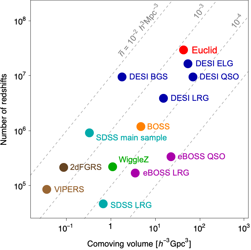
The Euclid NISP slitless spectroscopic survey is part of a new generation of such surveys, which will bring the total number of measured redshifts close to a hundred million. While Euclid will sample the redshift range from space, the DESI project (DESI Collaboration et al. 2016), already under way at the Kitt Peak 4-m Mayall telescope, is primarily targeting galaxies at lower redshifts (with significant overlap), using an innovative 5000-fibre automatic positioner. In fact, the wavelength range of its red grisms (Sect. 3.5.3) was specifically chosen as to make Euclid complementary to existing and planned ground-based surveys. The number of expected redshifts and the sampled volume of Euclid and DESI are compared with some previous surveys in Fig. 1.
The observed clustering of galaxies within a past lightcone encodes a wide range of physics through a number of processes. The currently favoured picture envisages that the initial comoving pattern of the overdensities that grew to form today’s galaxies and large-scale structures was set up in the early Universe, driven initially by inflation (e.g. Bassett et al. 2006). These were then modified before recombination, driven by physics that imprints scales related to the epoch of matter-radiation equality and the propagation of acoustic waves. These are commonly included in models of the power spectrum by a transfer function that multiplies the primordial power-law inflationary spectrum (e.g. Lewis et al. 2000). Shortly after recombination, the density contrast is still small over the scales of interest, perturbations are still linear and their growth is essentially scale-independent. Departures from scale-independence might thus signal the effects of non-zero neutrino mass (an effect of about one per cent is expected with current mass limits – see Lesgourgues & Pastor 2006, for a review), or more exotic physics. Starting from the smallest scales, at late times gravitational evolution becomes nonlinear, bringing in additional information, but also new complications (see, e.g. Bernardeau et al. 2002). As we discuss below, the way that pattern is imprinted into the angles and redshifts measured by a galaxy survey allows us to extract important cosmological information.
Much of this is encoded in the two-point statistics of the overdensity field: in configuration space,555With configuration space we mean the space where we measure galaxy positions and distances, dual to Fourier space. In turn, configuration space is distinguished into real space, where one uses true galaxy distances and separations are indicated with , and redshift space, where distances are derived from measured redshifts, and galaxy separations are typically indicated with . Correspondingly, the same distinction applies to the Fourier side, where wavenumbers can be defined in real and redshift space. Again, redshift-space quantities are usually indicated with the subscript . we measure the spatial two-point correlation function (2PCF) of galaxies, which quantifies the excess probability of finding two objects at a given separation with respect to a random Poisson sample tracing the same volume,
| (4) |
Here is the mean number of galaxies per unit volume and we are considering two small regions, separated by a vector , with volumes and , containing and galaxies, respectively. It is often convenient to measure clustering in Fourier space, and there we measure the power spectrum, which is the Fourier transform of the correlation function:
| (5) |
Our clustering computations use galaxy redshifts to derive their distances. However, redshifts include, in addition to the pure cosmological Hubble flow, the line-of-sight contribution of the galaxy peculiar velocities, induced by density inhomogeneities. This leads to coherent redshift-space distortion s (RSDs; Kaiser 1987), introducing an anisotropy in the observed clustering between line of sight (LoS) and transverse separations (see below for more details), such that we measure the clustering in redshift space with separations denoted by rather than . Hence, to properly describe (and model) this effect we typically measure the clustering with respect to the LoS. The cosmological information of interest is contained within the first three even power-law moments of the correlation function or power spectrum with respect to , under the global plane-parallel approximation, where is constant across a survey and gives the cosine of the angle that a pair of galaxies, for , or that the Fourier mode wave vector, for , makes with respect to the LoS. The first three even Legendre polynomials encode these power-law moments and form an orthonormal basis:
| (6) | |||||
| (7) | |||||
| (8) |
We therefore typically decompose the clustering into the Legendre polynomial moments of the correlation function and power spectrum (Hamilton 1998):
| (9) | ||||
| (10) |
with corresponding to the monopole, the quadrupole, and the hexadecapole moment. In practice, the LoS varies across a survey, and we typically make a local-plane parallel approximation, where we assume that the LOS is the same for each pair of galaxies analysed. In this case, the statistic we wish to measure is that given in Eq. 9, but the method by which we estimate it is not as simple as this equation suggests, as discussed in more detail in Sect. 7.7.1. A prediction for the power spectrum moments to be measured by Euclid is given in Fig. 2. This figure shows measurements on mock catalogues based on the Euclid Flagship simulation (see Sect. 6.1), and a best-fit model that is able to predict the clustering into the nonlinear regime (see Sect. 8.2.2 for more details).
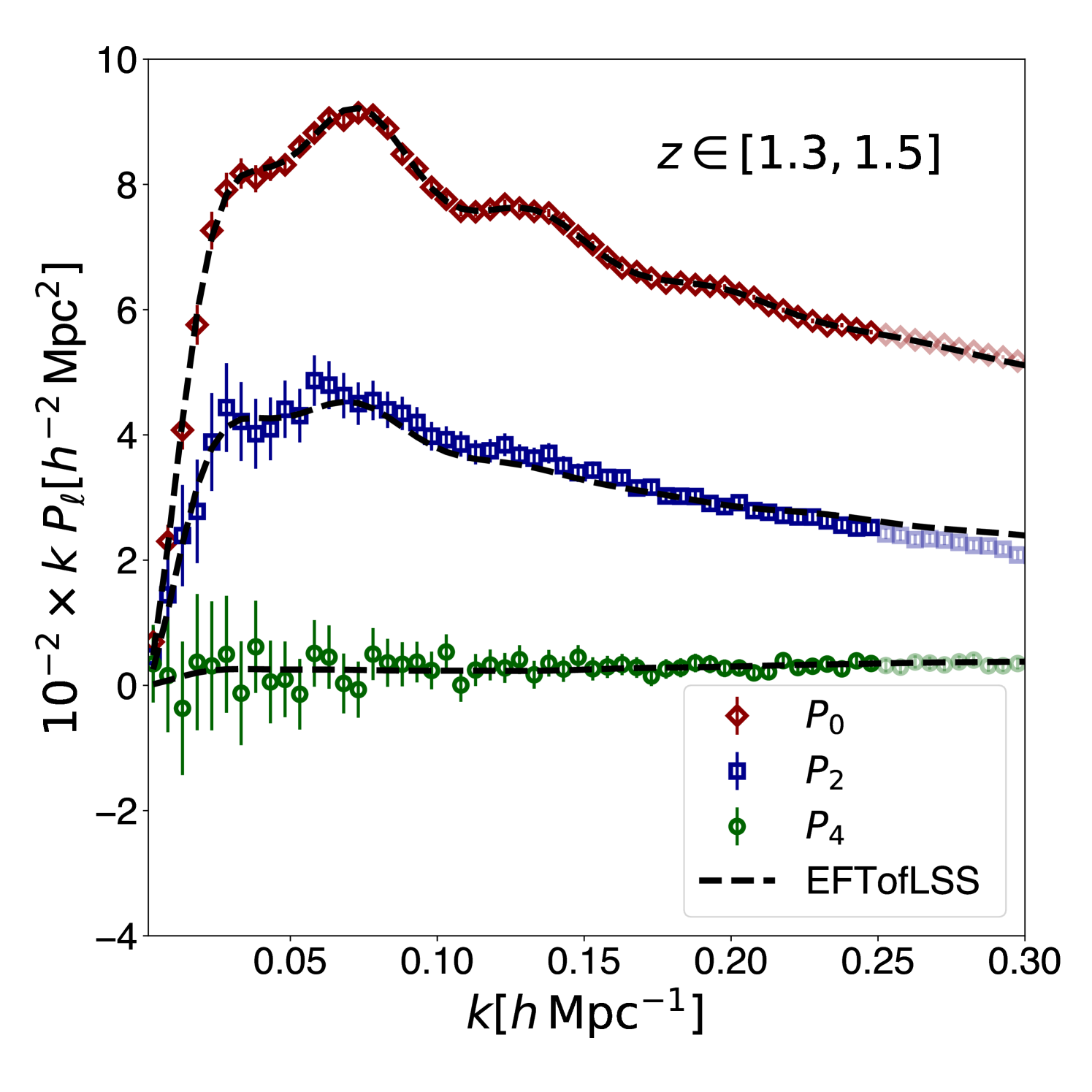
The most robust (and easy to isolate) signal in the pattern of galaxies are the so-called Baryonic Acoustic Oscillations (BAOs), a series of peaks and troughs in the power spectrum caused by acoustic waves during the pre-recombination era (e.g. Eisenstein & Hu 1998; Meiksin et al. 1999). These are evident in the monopole of Fig. 2. The acoustic waves push baryonic material out from initial perturbations to the baryon-drag scale, which is linked to the comoving sound horizon at recombination. When analysed in Fourier space this results in a sinusoidal term in the transfer function, depending on whether the movement of material cancels or reinforces that from other perturbations separated by the wavenumber of interest. The BAOs observed have the same physical origin as the oscillations seen in the CMB anisotropy power spectrum (Planck Collaboration VI 2020), and were first observed in the 2dFGRS (Percival et al. 2001; Cole et al. 2005) and SDSS (Eisenstein et al. 2005) surveys. Hardware improvements made to the Sloan telescope enabled BOSS to provide the first 5 measurement of BAOs from the largest volume of the Universe obtained at that point (Anderson et al. 2012). The extended-BOSS project pushed these BAO observations to higher redshifts (Alam et al. 2021). The BAO are largely insensitive to galaxy bias, simplifying their modelling.
The power of BAOs in a galaxy survey results from using them as a standard ruler undergoing expansion that is comoving with the average expansion of the Universe. The observed wavenumbers of BAOs constrains the ratio in the radial direction, and in the transverse direction, where is the sound horizon at the end of the drag epoch, is the Hubble distance, and is the angular-diameter distance. The different dependencies along and across the LOS lead to a very clean geometrical measurement: the correct set of cosmological parameters will be the one leading to a statistically isotropic clustering requiring the product to match the truth. This is known as the Alcock-Paczynski (AP; Alcock & Paczynski 1979) effect and the principle holds for features in the power spectrum other than BAOs; for example it can also be applied to stacks of objects such as voids, which are under-dense regions defined by a specific threshold (see Pisani et al. 2019, for a review). With the unprecedented volume of the Wide survey, void statistics with Euclid, such as the void size function and the void-galaxy cross-correlation function are expected to deliver competitive, complementary cosmological constraints (see Verza et al. 2019; Hamaus et al. 2022; Contarini et al. 2022; Bonici et al. 2023; Radinović et al. 2023, for specific forecasts).
The BAOs are just one feature within the full power spectrum of the galaxy distribution. The shape of the galaxy power spectrum underlying the BAO depends on cosmology through the spectral index of the fluctuations coming from inflation and the matter-radiation horizon scale, which depends on the parameter combination . The full power spectrum predicted to be observed by Euclid is shown in Fig. 2 in terms of its Legendre multipoles.
While BAOs carry information about the expansion history and thus the equation-of-state parameter of dark energy , the anisotropy of the clustering pattern produced by RSDs, mentioned earlier, provides us with complementary, potentially powerful information on the growth rate of structure . As discussed in the introduction to this section, combined precise measurements of and are key to understand the origin of cosmic acceleration, potentially discriminating between dark energy and modifications of GR, a major goal of Euclid. The confidence in the use of RSDs as a test of dark energy consolidated at the time of the ESA Cosmic Vision 2020-2025 call (Guzzo et al. 2008; Wang 2008a). In fact, the use of RSDs as a primary cosmological probe was one key original ingredient in the SPACE proposal (Cimatti et al. 2009), which eventually became the spectroscopic experiment on board Euclid (also see Wang et al. 2010). Since then, virtually all redshift surveys have been including RSDs as a standard probe of the growth rate of structure (see Alam et al. 2017, 2021, and references therein). In practice, the growth rate is derived from RSDs by modelling the measured anisotropy of the correlation function or power spectrum, as quantified by their multipoles, which depends on the combination (Percival & White 2009).
In galaxy clustering measurements, is degenerate with the so-called ‘galaxy bias’, that is the unknown amplification with respect to the clustering of the underlying matter density field. This is expected to arise naturally if galaxies form at the peaks of the density-fluctuation field (Kaiser 1984), with additional complications and scale-dependence on small scales (see Desjacques et al. 2018, for an extensive review). There, comoving galaxy separations no longer match those between the seed perturbations from which their hosting dark matter halos grew. Galaxy formation and evolution inside halos adds a further layer of complication, that is a galaxy-halo bias. On very large scales the galaxy bias signal can depend on the level of primordial non-Gaussianity, typically enabling a measurement of the parameter. Except for the deviation caused by the signal, we expect the large-scale bias of galaxies to tend towards the scale-independent deterministic linear value predicted by a pure statistical peak (halo) to background (matter) bias. In that case the galaxy power spectrum is simply proportional to the matter power spectrum, .
The statistical properties of a Gaussian random field are completely described by its two-point correlation function or, equivalently, the power spectrum. This is not the case for the galaxy distribution which is highly non-Gaussian as it is shaped by several nonlinear processes, such as gravitational instability, redshift-space distortions, and galaxy biasing. Higher-order clustering statistics, starting from the galaxy three-point function in configuration space, or the bispectrum in Fourier space, are the direct result of these nonlinear effects. Recent studies have demonstrated that performing a joint analysis of two- and three-point statistics of the galaxy distribution is key to disentangling the impact of these nonlinearities from the signatures of new physics. This is expected to improve constraints on the cosmological parameters by 10-30% (Yankelevich & Porciani 2019). In addition, there are models of inflation that can only be constrained using higher-order statistics (e.g. D’Amico et al. 2022). To take advantage of this additional information, we will measure the redshift-space multipoles for both the three-point function and the bispectrum (also see Sect. 9) and analyse them jointly with two-point statistics as a natural extension of all probes and methods mentioned above.
The signatures of the physical processes discussed above can lead to strong degeneracies between measurements, for example, between the AP effect and RSDs (Ballinger et al. 1996). Thus it is important to measure them together, and to mitigate the effects of galaxy bias (see Sect. 8.2.2). The relative robustness of using the BAO signature as a standard ruler means that it is often advantageous to extract this information separately. This is commonly achieved by fitting a model where polynomial or similar terms are added in order to isolate the BAO feature in the power spectrum (Beutler et al. 2017) or correlation function (Ross et al. 2017). The scale of the BAO signal is then extracted and used directly to constrain models. The precision with which the BAO scale can be measured can be improved by a technique called reconstruction (Eisenstein et al. 2007), where the nonlinear motions of galaxies are estimated from the galaxy field, and used to find the positions of the initial overdensities. This sharpens the BAO signal, increasing the precision of the determination of the centroid.
The galaxy-clustering probe uses overdensities in the galaxy field as a direct probe of cosmology and thus is sensitive to non-cosmological effects that alter observed densities. In order to use galaxy surveys one has to understand their specific selection function, so as to define a mask or window that describes where galaxies can be found. Typically, because of the windows’ complexity, this is usually quantified by making use of random catalogues, Poisson sampling the expected density. The overdensity is then extracted by comparing galaxy and random catalogues (see Sect. 7.7.1 for a description of how these will be created). Typical problems in the analysis of galaxy surveys arise from the selection of the galaxy sample, which can be distorted by Galactic extinction or stellar density (Ross et al. 2012). For example, areas near bright stars are unusable and must be masked. If these changes in the observed density are not corrected by matching the weighted galaxy field to the weighted random field, then the spatial distribution of bright stars may be imprinted in the overdensities in our map of the Universe and misinterpreted as a cosmological signal. Space-based slitless spectroscopy helps to reduce the impact of many of these effects. In particular, no target sample is required to be selected from ground-based imaging data. On the other hand, this requires careful understanding of the potential density-dependent systematic effects that could arise due to confusion among faint spectra in crowded areas. Considerable effort has been invested to understand and model these effects through end-to-end simulations.
The cosmological information available from the galaxy field is simplest to extract where the physics can be explained by linear processes. On small scales, gravity induces nonlinearities in the distribution of density. It is possible that by studying particular locations in the density field, such as voids or clusters, the linear information on small scales may be easier to extract than from the field as a whole. For example, the relation between the overdensity and velocity field near voids is thought to be close to linear (Hamaus et al. 2014). For the AP effect, we can extract additional information from the fact that a stack of voids should be spherical on average (e.g. Woodfinden et al. 2023). Thus, in addition to the galaxy field, Euclid will study these special places in the Universe to obtain further, complementary cosmological information.
2.2 Weak gravitational lensing
As demonstrated in the previous section, galaxies are powerful, but biased, tracers of the LSS. To fully exploit the statistical power of the density modes traced by the galaxies, we need to link their properties to the surrounding matter structures. Hence, a direct measurement of the (predominantly dark) matter distribution provides not only important information on how galaxies populate halos, but also probes the growth of large-scale structures. Conveniently, such a measurement is possible thanks to the observable effects of gravitational lensing: massive structures distort space-time, warping the paths of photons. If the deflections are sufficiently large, multiple images of distant galaxies are formed. Such cases of strong gravitational lensing can be used to study the matter distribution on small scales, or exploited as cosmic magnifying glasses (see Sect. 9.3 for some applications).
Generally, the deflections of single objects cannot be measured. However, the matter distribution, via its tidal gravitational field, gives rise to small coherent distortions in the shapes of distant galaxies. This change in the observed galaxy shapes is called weak gravitational lensing (for thorough introductions, see Mellier 1999; Bartelmann & Schneider 2001; Bartelmann 2010). In particular, the weak lensing shear, which describes the weak lensing-induced difference in the galaxies’ observed ellipticity 666As is common in the weak lensing literature, we refer to the quantity describing the shape of a galaxy as ‘ellipticity’. Mathematically, this ellipticity corresponds to the third flattening of the galaxy image. contains information on the cosmic matter distribution. This shear is small compared to the intrinsic ellipticities of galaxies, and ensembles of galaxies need to be averaged to reveal the coherent patterns that can be used to map the distribution of matter along the LoS (Kaiser & Squires 1993, also see Sect. 7.7.3). The weak lensing signal was first detected around massive clusters of galaxies (Tyson et al. 1990) and its potential for cosmology was quickly recognised (e.g. Blandford et al. 1991; Miralda-Escude 1991; Kaiser 1992; Bernardeau et al. 1997) as the shape correlations provide statistical information about the cosmic LSS, which, in turn, depends on the cosmic expansion history and structure growth (see e.g. Kilbinger 2015, for a recent review). This led to the first deep imaging campaigns to measure weak lensing by LSS, or cosmic shear, with the first unambiguous detections reported nearly simultaneously by Bacon et al. (2000), Kaiser et al. (2000), Van Waerbeke et al. (2000), Wittman et al. (2000). Since then, weak lensing has become an established tool to infer cosmological parameters and has been successfully applied to ever larger surveys, such as the Hyper Suprime-Cam (HSC; Aihara et al. 2018), the Kilo-Degree Survey (KiDS; Kuijken et al. 2015), and the Dark Energy Survey (DES; Abbott et al. 2016; Becker et al. 2016).
The weak lensing signal can be decomposed into a curl-free -mode and a gradient-free -mode component (Crittenden et al. 2002; Schneider et al. 2002a). To first order, weak lensing by the LSS only causes -modes, while -modes can be caused by systematic and astrophysical effects (e.g. Heavens et al. 2000; Schneider et al. 2002b; Hoekstra 2004). Usually, the -mode signal is used for cosmological analysis, while the -mode signal is a probe of unmodelled systematic effects (e.g. Hildebrandt et al. 2017; Asgari & Heymans 2019).
For cosmic shear studies, key observables are the two-point shear correlation functions and , which correlate the estimates for the shear components of pairs of distant galaxies at angular positions and , respectively, so that
| (11) |
where and are the tangential and cross-component of the shear, defined with respect to the separation between the galaxies. The shear correlation functions are related777To simplify the discussion, we ignore the fact that the observed ellipticities provide an estimate for the reduced shear , where is the convergence (see e.g. Schneider & Seitz 1995; Bartelmann & Schneider 2001, for more details). We also implicitly ignore intrinsic alignments. In the actual analysis of Euclid data, these, and several other subtle complications, will need to be accounted for (Euclid Collaboration: Deshpande et al. 2024). to the - and -mode shear power spectra and as (Chon et al. 2004; Lemos et al. 2017; Kilbinger et al. 2017; Kitching et al. 2017)
| (12) |
where is the Wigner- function. In turn, is related to the matter power spectrum . Under the flat-sky approximation this relation reduces to Hankel transforms,
| (13) |
where the are Bessel-functions of the first kind and is used for and for . Neglecting -modes, a simple form of the relation between and can be derived by assuming the Limber approximation (Limber 1953; Kaiser 1998), and a spatially flat Universe (see Taylor et al. 2018b, for a generalisation beyond this assumption) as
| (14) |
where the prefactor,
| (15) |
comes partly from the conversion from the spectrum of the lensing potential to that of shear modes, and partly from the Limber approximation (see Lemos et al. 2017; Kilbinger et al. 2017; Kitching et al. 2017, for derivations of these expressions, and relaxation of the approximations). Above, is the comoving distance at redshift , and is the lensing efficiency kernel,
| (16) |
for a sample of sources with a redshift distribution .888Note that has to be normalised to unit area, that is, . Hence, the interpretation of the observed lensing signal depends on knowing the redshift distribution of the source galaxies. Although redshifts for individual galaxies are not required, the sensitivity to cosmological parameters is rather limited when a single set of sources is used.
To exploit the information on the evolution of the LSS over cosmic time, key to constraining the dark energy equation of state parameter, , the sources need to be divided into narrow redshift bins that, ideally, do not overlap. Combined, the bins provide tomographic information on the matter distribution along the LoS. A finer tomographic binning increases the redshift resolution, but also leads to a decrease of the signal-to-noise ratio in each individual bin as it contains fewer galaxies. Moreover, as the sources in different bins probe the same structures at lower redshifts, the resulting lensing signals are highly correlated, and the statistical gain saturates quickly (Ma et al. 2006).
A tomographic analysis requires redshift estimates for the individual sources, which are too faint and too numerous for dedicated spectroscopic follow-up. Fortunately, photometric redshifts (Koo 1985; Loh & Spillar 1986; Newman & Gruen 2022) can be used, provided their precision is substantially better than the width of the tomographic bins. In the case of Euclid, we aim to divide the source sample into as many as 13 bins in the range . To achieve these objectives, the standard deviation of the photometric redshift estimates needs to satisfy , while the catastrophic failure rate needs to be less than 10% (Amara & Réfrégier 2007; Laureijs et al. 2011). To meet these stringent requirements, Euclid complements the VIS data with deep space-based near-infrared (NIR) photometry in three bands; we also take additional, uniform photometry from the ground (see Sect. 4.4). Moreover, to obtain accurate cosmological parameter estimates, the mean galaxy redshifts within the bins need to be known with an accuracy (Ma et al. 2006; Amara & Réfrégier 2007; Kitching et al. 2008b). As discussed in more detail in Sect. 7.6.1, this drives the need for extensive spectroscopy that fully samples the colour-redshift space (e.g. Masters et al. 2015).
Such relatively narrow redshift bins offer a powerful handle on the time evolution of the cosmic shear spectra. It allows us also to take full advantage of the so-called Bernardeau–Nishimichi–Taruya (BNT) transformation (Bernardeau et al. 2014; Taylor et al. 2018a, 2021, also see Sect. 8) with which scale mixing from projection effects can be fully controlled. This has major benefits for the interpretation of the weak lensing signal from theoretical models and the modelling of astrophysical systematic effects (Taylor et al. 2021). Another motivation for the fine binning is the need to combine the lensing measurements with the angular positions of galaxies in a so-called ‘3×2pt’ analysis, discussed in Sect. 2.3.
The shear correlation functions (and convergence power spectra) primarily depend on the square of the parameter in the linear regime, and to higher orders of at smaller scales. (e.g. Hall 2021). The degeneracy between and is broken by nonlinear corrections or with the use of higher-order statistics (Bernardeau et al. 1997). Cosmic shear analyses of current surveys at the time of writing have already tightly constrained with a precision of (e.g. Asgari et al. 2021; Amon et al. 2022; Li et al. 2023b). Interestingly, the reported values are consistently lower than the one inferred from the cosmic microwave background with Planck. The current level of disagreement for individual measurements ranges from 2 to , but it remains to be seen if this points to a problem with the cosmological standard model (Di Valentino et al. 2021).
Cosmic shear is also sensitive to the cosmic expansion history and the dark energy equation of state through the angular-diameter distances between the observer, the distorted source galaxies, and the lensing matter structures; changes in the projection of structures along the LoS; and the decay in gravitational potentials as the expansion accelerates. Current cosmic shear analyses lack the statistical constraining power to provide meaningful constraints on the dark energy equation of state. This will change with Euclid, since it will achieve more than an order-of-magnitude increase in precision compared to previous surveys (Euclid Collaboration: Blanchard et al. 2020), owing to its depth, precise shear measurements, large area, and high galaxy density.

The statistical uncertainty of weak lensing measurements is primarily limited by sample variance and shape noise, both of which will be immensely reduced by Euclid. The Euclid Wide Survey (EWS, see Sect. 4) will cover an area 3 times larger than the final DES release, the largest deep imaging survey to date, suppressing sample variance. Additionally, since Euclid has greater depth than previous surveys, it effectively probes a larger volume of the Universe. Euclid is expected to detect about 2 billion source galaxies for which shapes can be measured, several orders-of-magnitude more than current surveys, thereby reducing shape noise. Given that many of these galaxies are at higher redshifts than those used in previous surveys, the observed galaxies typically exhibit larger lensing signals, further enhancing the signal-to-noise ratio. These strengths, particularly its depth, accurate shear measurements, and large galaxy numbers, will help Euclid to achieve a significant increase in precision compared to previous surveys (see Amara & Réfrégier 2007, for the scaling of the FoM with these survey parameters), while the sharp point spread function (PSF) reduces the detrimental impact of blending on the shape measurements (MacCrann et al. 2022; Li et al. 2023a).
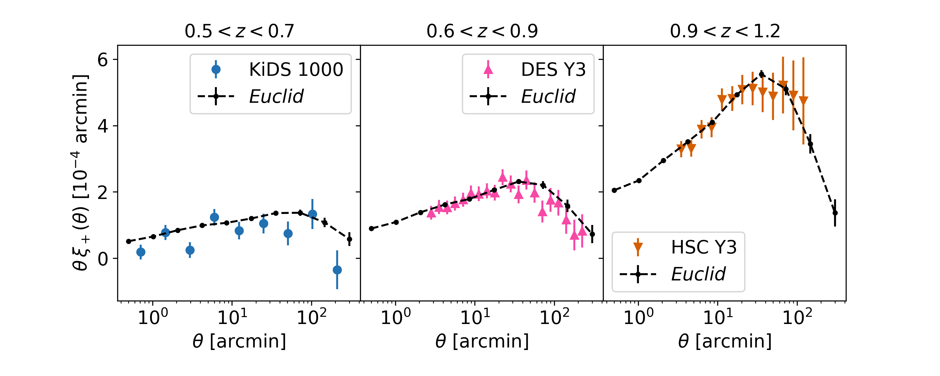
This is illustrated in Fig. 3, where we show shear correlation functions measured by the KiDS (Asgari et al. 2021), DES (Amon et al. 2022), and HSC (Li et al. 2023b). Each panel shows for the tomographic bin with the highest S/N for each survey. Error bars are the square root of the diagonal elements of the cosmic shear covariances, including shape noise and sample variance. For Euclid, these were computed with the OneCovariance-code999https://github.com/rreischke/OneCovariance; it uses the same prescription as Joachimi et al. (2021), which is similar to Euclid Collaboration: Sciotti et al. (2023) and Upham et al. (2022) (Reischke et al., in prep.). Comparing with the predictions for Euclid in the same tomographic bin, we expect an order of magnitude increase in S/N thanks to the combination of a higher galaxy number density and the increase in survey area.
The increase in galaxy number density is also apparent from Fig. 4, which demonstrates another advantage of Euclid compared to previous surveys, namely its increased redshift range. The amplitude of the lensing signal rapidly increases as a function of source redshift (Bernardeau et al. 1997), so that even a modest increase in number density of higher redshift sources can lead to a significant improvement in constraining power. The figure compares the redshift distribution of KiDS (Hildebrandt et al. 2021), DES (Myles et al. 2021), and HSC (Rau et al. 2023), to the expected redshift distribution for Euclid, obtained by selecting galaxies with in the Flagship 2 simulation (see Sect. 6.1). Shape measurements in KiDS and DES are essentially limited to galaxies at . The deep HSC data allow for a significant number of galaxies at redshifts between 1 and 1.5, but only Euclid will obtain a meaningful number of sources at higher redshifts. This larger redshift range is crucial for determining the evolution of dark energy.
To exploit the unprecedented statistical power of Euclid, it is essential that instrumental sources of bias are much smaller than the measurement uncertainties. Moreover, the exquisite measurements need to be complemented with accurate modelling of cosmological and astrophysical effects. Systematic effects for weak lensing arise, for example, from imperfect shape measurements and biases in the estimation of the source redshift distribution. We refer the interested reader to the review by Mandelbaum (2018) for a more in-depth discussion.
The observed images are modified by the telescope optics: even for space-based observations the blurring by the PSF is a dominant source of bias that needs to be accounted for. Moreover, imperfections in the detector introduce additional changes in the images, while cosmic rays pose another challenge. Considering the estimated shear and the true shear as complex numbers, their difference can be expressed to first order (see Kitching et al. 2020) as
| (17) |
where and are spin-0 and spin-4 complex operators, respectively, and the asterisk denotes complex conjugation. The value of quantifies the dilation and rotation of the true shear, whereas allows for a reflection around the axis determined by its phase (Euclid Collaboration: Congedo et al. 2024). is the additive bias, while corresponds to the random (shape) noise in the shear estimate.
The biases depend on the instrument, the shape measurement method (e.g. Heymans et al. 2006; Hoekstra et al. 2017, 2021), and galaxy properties, in particular the size and signal-to-noise ratio (e.g. Hoekstra et al. 2015). They can also vary spatially, but is affected principally only by the mean multiplicative bias101010Recently, Kitching & Deshpande (2022) highlighted that any nonlinearity in the relation between the true and estimated shear needs to be quantified and possibly accounted for. and the correlation between the shear field and the additive bias (Kitching et al. 2019, 2021).
Given a survey design, it is possible to derive limits on the shear biases that can be tolerated (Amara & Réfrégier 2008). These can be specified further by exploring how errors in the estimate of the PSF propagate (Paulin-Henriksson et al. 2009; Massey et al. 2013), as well as other sources of bias. The detailed breakdown presented in Cropper et al. (2013) formed the basis for the development of the shape measurement pipeline for Euclid, which is discussed in more detail in Sect. 7.6.
To realise the full statistical potential of Euclid, we require the uncertainty on the multiplicative bias to be less than , and the uncertainty on the additive bias to be less than (Cropper et al. 2013). Recent studies (Euclid Collaboration: Paykari et al. 2020; Kitching et al. 2019) have shown that we need to distinguish between sources of bias that are constant across the survey and spatially varying effects. Although these refinements can provide margin for specific instrumental effects, the baseline requirements provided an excellent basis for the hardware and software development needed for the mission.
Because we aim to push the limits of what can be done within the mission constraints, the measurements are challenging, despite the advantages that a space telescope brings. Compared to ground-based surveys the main benefit of Euclid is that the PSF residuals scale with the square of the PSF size (Paulin-Henriksson et al. 2009; Massey et al. 2013). This reduces the baseline multiplicative bias for Euclid compared to ground-based telescopes, which cannot avoid the blurring of the images by atmospheric turbulence. Nonetheless, the PSF needs to be known with unprecedented accuracy. A complication is that we need to account for the fact that the PSF is a strong function of wavelength, and therefore depends on the spectral energy distribution (SED) of each individual galaxy (Cypriano et al. 2010; Eriksen & Hoekstra 2018), which can also vary spatially (Voigt et al. 2012; Semboloni et al. 2013a; Er et al. 2018). The challenges in modelling the PSF and measuring the shapes of galaxies are discussed in Sects. 7.6.4 and 7.6.5, respectively.
Since the weak lensing observables provide unbiased estimates of the projected matter distribution, it was believed that the interpretation of the lensing signal would be relatively immune to astrophysical processes. However, it has become clear that this is not the case, especially at the precision of Euclid. First of all, the intrinsic shapes of galaxies are correlated with each other and their surrounding matter distribution due to tidal interactions during their formation. This intrinsic alignment (IA) effect needs to be accounted for, because it causes spurious signals in the cosmic shear signal and the position-shear correlations (Joachimi et al. 2015; Kirk et al. 2015; Troxel & Ishak 2015). On large scales, tidal alignment models provide a description of the scale dependence (e.g. Hirata & Seljak 2004; Bridle & King 2007; Blazek et al. 2019), but the amplitude of the IA signal cannot be predicted from first principles because it depends on the complex process of galaxy formation. Moreover, the signal depends on galaxy type, galaxy luminosity, and redshift. Although observations can be used to constrain the predicted amplitude (Fortuna et al. 2021), our current knowledge of the IA signal is insufficient. Euclid itself will be a great resource for direct measurements, but the modelling of the IA signal is likely to remain an active area of research for the foreseeable future.
The second complication is that non-gravitational processes, such as heating by active galactic nuclei, supernovae, or star formation, redistribute baryons. To explain current observations, models of galaxy formation require that a significant fraction of the baryons are expelled, leading to a suppression of the matter power spectrum (van Daalen et al. 2011; Debackere et al. 2020). Neglecting these processes can significantly bias cosmological parameter constraints (e.g. Semboloni et al. 2011, 2013b; Chisari et al. 2019). In principle, the changes in the matter distribution can be modelled using hydrodynamical simulations (e.g. Schaye et al. 2010, Le Brun et al. 2014, McCarthy et al. 2017), physically motivated modifications to analytical halo models (e.g. Debackere et al. 2020, Mead et al. 2021), or ‘baryonification’ models that modify halos in gravity-only simulations according to prescribed gas content (Schneider & Teyssier 2015, Schneider et al. 2019, Aricò et al. 2020). The challenge is to decide which models capture the feedback processes correctly, although the findings of van Daalen et al. (2020) suggest it may be possible to describe the effect of feedback on the matter power spectrum with only a few nuisance parameters that need to be marginalised over when estimating the cosmological parameters. Finally, several simplifying assumptions in the modelling of the observed cosmic shear power spectrum need re-evaluation for Euclid, such as an increased source galaxy density due to weak lensing magnification (magnification bias), the exclusion of blended galaxy pairs (source obscuration), and local over- or under-densities (Euclid Collaboration: Deshpande et al. 2024).
2.3 Photometric 3×2pt analysis
Although cosmic shear is a powerful probe of cosmology, it cannot reach a by itself (Laureijs et al. 2011; Euclid Collaboration: Blanchard et al. 2020). To unlock the full constraining power of Euclid, we need to combine the cosmic shear correlation functions, , with the galaxy angular correlation function, , and the cross-correlations between galaxy angular positions and the tangential component of the ellipticities of background galaxies, . These additional two-point functions are commonly referred to as ‘photometric galaxy clustering’ and ‘galaxy-galaxy lensing’ or ‘shear-clustering cross-correlation’, respectively.
Equivalently, angular power spectra can be measured and used for the analysis. Hence, Eq. 14 can be generalised to encompass all three probes,
| (18) | ||||
In the expression above, and label the probes being correlated, while and indicate the tomographic bins considered. In the case of shear, is given by Eq. 15, whereas . For instance, for and , we obtain Eq. 14. Alternatively, it is possible to include intrinsic alignments by using the ellipticity power spectrum (Euclid Collaboration: Blanchard et al. 2020). For photometric galaxy clustering, we take and, assuming a linear galaxy bias,
| (19) |
while and corresponds to the shear-clustering cross-correlation. Note that the galaxy bias, , will in general be different from that of the galaxies in the spectroscopic sample discussed in Sect. 2.1. Moreover, as mentioned in this subsection, the (binned) redshift probability distribution of sources, , used for clustering might differ from that employed for cosmic shear.
A combined analysis including all of such correlations is commonly referred to as a ‘pt analysis’. It can significantly enhance the constraining power: for Euclid the FoM is increased by roughly a factor 20, relative to a cosmic-shear-only scenario (Tutusaus et al. 2020; Euclid Collaboration: Blanchard et al. 2020). Hence, it should not come as a surprise that such an approach has become the standard for current surveys (e.g. van Uitert et al. 2018; Joudaki et al. 2018; Abbott et al. 2018a, 2022; More et al. 2023). Additional cross-correlations, for instance with CMB measurements (Sect. 9.4), can be included for pt analyses (e.g. Abbott et al. 2019, 2023).
The benefit of combining these three types of correlations lies in their ability to lift degeneracies between parameters (both cosmological and nuisance), such as the galaxy bias parameters that are needed to describe how galaxies trace the underlying matter distribution. In contrast, galaxy clustering is not affected by intrinsic-alignment and shape-measurement biases. Moreover, the clustering-shear cross-correlation is subject to the same systematic effects as cosmic shear and galaxy clustering, but has a different functional dependence. Combining these probes allows for the partial self-calibration of systematic effects (Bernstein & Jain 2004; Hu & Jain 2004; Bernstein 2009; Joachimi & Bridle 2010). This self-calibration enables tight control over systematic effects. Thus, the main cosmic shear cosmological results from Euclid will be derived from a pt analysis, made possible by the precise weak lensing measurements. In the cosmological parameter forecasts in Sect. 8.2.3, we present the expected parameter constraints from this analysis.
The improved constraining power comes at a price: we need to accurately measure and consistently model a larger number of probes. In principle, photometric clustering includes all the physical effects described in Sect. 2.1, including BAOs and RSDs. However, given the lack of resolution along the LoS, the information is generally projected within each tomographic bin, similar to what is done for weak lensing. By limiting the analysis to the angular correlation function between galaxies, most of the RSD signal is lost (although not completely, see Euclid Collaboration: Camera et al., in prep.). However, we need to include RSDs in the modelling in order not to bias our cosmological results (e.g. Euclid Collaboration: Tanidis et al. 2024).
Moreover, thanks to the low radial resolution of this probe, the BAO signal is partially smoothed out and therefore we can use smaller scales than those considered in spectroscopic clustering analyses, even if our model is not as accurate. As a result, most of the information from photometric galaxy clustering comes from scales slightly smaller than those used in Sect. 2.1, making them complementary probes. We note, however, that photometric galaxy clustering still uses biased tracers; therefore, we cannot use scales as small as for weak lensing, given the difficulty in modelling the galaxy bias at small scales. Another physical effect that needs to be included in the modelling of the signal is magnification. This lensing effect does not add much constraining power (Mahony et al. 2022), but ignoring its impact on the clustering signal leads to biased parameter estimates (see e.g. Duncan et al. 2022; Euclid Collaboration: Lepori et al. 2022; Martinelli et al. 2022). For galaxy-galaxy lensing, all these effects also need to be considered, in addition to those relevant for weak lensing.
A robust measurement of photometric clustering poses new challenges, in part owing to its reliance on ground-based data that were obtained under varying observing conditions. If these variations are not accounted for, they can lead to spurious clustering (Ross et al. 2011; Elvin-Poole et al. 2018; Johnston et al. 2021; Rodr´ıguez-Monroy et al. 2022). Further complications arise from contamination by stars and Galactic extinction, or zodiacal light, which can change the galaxy counts on relatively large scales. In principle, these contributions are included in the visibility mask (see Sect. 7.7.2), which is used to correct the measurements. Work to optimise the galaxy samples is ongoing. In particular, it may be advantageous to consider samples of bright galaxies, which are more immune against spurious clustering.
3 Spacecraft and instruments
The primary cosmological probes of Euclid’s core science case have defined the main survey characteristics (Sect. 4), as well as the requirements for the capabilities of the telescope and instrument. Besides a maximum cost, in accordance with its ‘medium’ mission size, ESA imposed a so-called technology readiness level of 5 or higher for the components of the proposed mission. This restriction allows only the use of technologies that have already been validated in the relevant environment.
Before Euclid’s final design and scope were defined, initial assessment studies with industry and the science community resulted in a set of feasible science and mission requirements. The subsequent definition phase provided a detailed description of the scientific scope based on a mission design that could be developed within the programmatic constraints set by ESA (Laureijs et al. 2011). After its selection in 2011, the Euclid mission was adopted by ESA’s science programme committee in June 2012, to enter the implementation phase with industrial contracts for the development of the space segment and with a multilateral agreement between ESA and the participating countries for the delivery of the two science instruments and the development of the science ground segment.
Euclid was originally planned to be launched on a Soyuz ST-2.1B rocket (Laureijs et al. 2011), but the geopolitical developments that unfolded in 2022 resulted in the cancellation of this possibility. Investigations revealed that a SpaceX Falcon-9 could provide a suitable alternative, which was ultimately confirmed with the successful launch on 1 July 2023 into an orbit around the second Lagrange point of the Sun-Earth system (hereafter L2). This orbit provides a thermally stable environment with unobstructed views of the sky, prerequisites for a successful use of the planned cosmological probes. The most salient details about the spacecraft are presented in Sect. 3.1. Information about the transfer into the halo orbit around L2 and orbital maintenance is provided in Sect. 3.2, while pointing constrains are discussed in Sect. 3.3.
The spacecraft contains two main science instruments: the visible imaging instrument (VIS; Sect. 3.4); and the Near Infrared Spectrometer and Photometer (NISP; Sect. 3.5). Both instruments were designed to provide high-quality data over a wide field of view (FoV) with a high degree of accuracy and precision. The resulting homogeneous, high-quality space-based observations benefit from the thermally very stable environment, and from the absence of atmospheric blurring and bright sky background, providing a data set of unrivalled fidelity.
3.1 Spacecraft
The Euclid spacecraft can be subdivided into three main parts: the service module (SVM); the payload module (PLM) including the telescope; and the scientific instruments (called collectively ‘extended PLM’). The design of the spacecraft is described in detail by Racca et al. (2016); here, we present a summary overview and the most important changes until launch, and observations during the commissioning phase.
| Component | Mass [kg] |
|---|---|
| Service module (SVM) | 901.0 |
| (Warm instrument units) | (64.5) |
| Payload module (PLM) | 806.4 |
| (Cold instrument units) | (156.4) |
| Propellant ( and ) | 210.7 |
| Launch vehicle adaptor and clamp band | 70.0 |
| Total launch mass | 1988.1 |
3.1.1 Service module
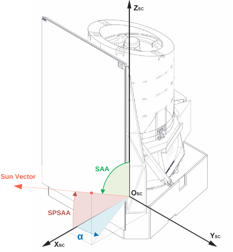
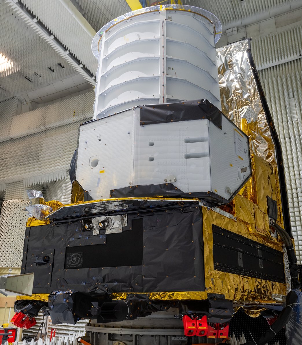
The SVM comprises the spacecraft subsystems supporting the payload operations; it hosts the warm electronics of the payload, and provides structural interfaces to the PLM and the launch vehicle. The prominent sunshield is part of the SVM. It protects the PLM from illumination by the Sun and supports the photovoltaic assembly supplying electrical power to the spacecraft. On top of it, a triple blade sun-baffle is mounted with the purpose to reduce the sunlight diffracted towards the PLM baffle aperture. The overall spacecraft envelope fits within a diameter of 3.74 m and a height of 4.8 m. Euclid’s total launch mass budget, including propellant for operations, is 1988.1 kg (see Footnote 11). The left panel in Fig. 5 shows an overview sketch of Euclid in launch configuration, including the definition of its axes, while the right panel shows the fully assembled spacecraft during testing in February 2023.
3.1.2 Payload module
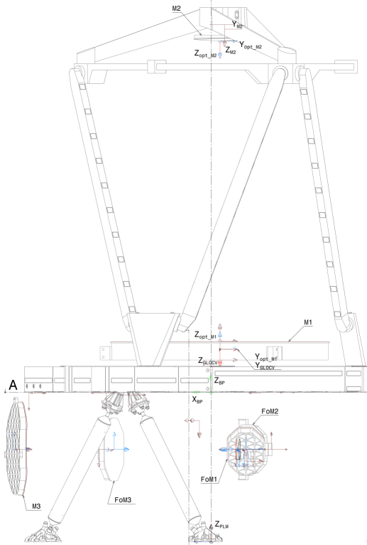
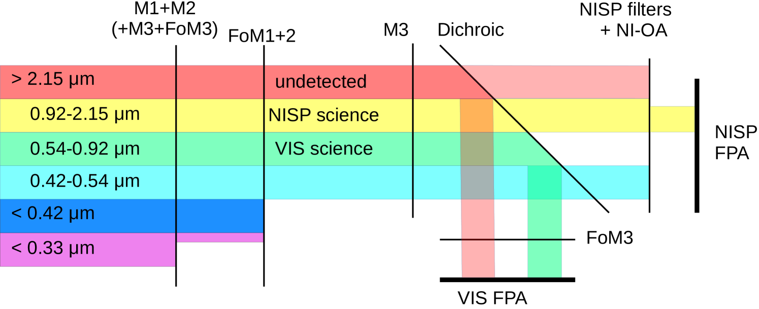
The Euclid PLM is designed around a three-mirror anastigmat Korsch telescope (Korsch 1977) with a 1.2-m primary mirror and an effective collecting area of 0.9926 m2 (Gaspar Venancio et al. 2014). The telescope provides a common area between instruments of about 0.54 deg2 with minimal spherical aberration, astigmatism, coma, and field curvature. The mirrors and telescope structure are made from silicon carbide (SiC; Bougoin et al. 2019), with the optical path schematically shown in Fig. 6. The light separation between the two instruments is performed by a dichroic plate located at the exit pupil of the telescope. The PLM provides the mechanical and thermal interfaces to the instruments, consisting of radiating areas and heating lines.
Whereas NISP is a stand-alone instrument with interface bipods, VIS is delivered in several separate parts. It consists of a focal plane assembly (FPA) containing all detectors, connected to proximity electronics, readout shutter unit, and calibration unit, each with their own dedicated mechanical and thermal interfaces with the PLM.
The secondary mirror (M2) is mounted on the M2 mechanism (M2M), allowing adjustment in three degrees of freedom for focusing and some optical alignment. In addition, the PLM hosts the fine-guidance sensors (FGSs), used as pointing reference by the attitude and orbit-control system (AOCS). The FGS detectors are mounted on the same structure carrying the VIS focal plane to ensure precise co-alignment. Except for the proximity electronics of the VIS and FGS focal planes, all electronics are placed on the SVM to minimise thermal disturbances of the PLM.
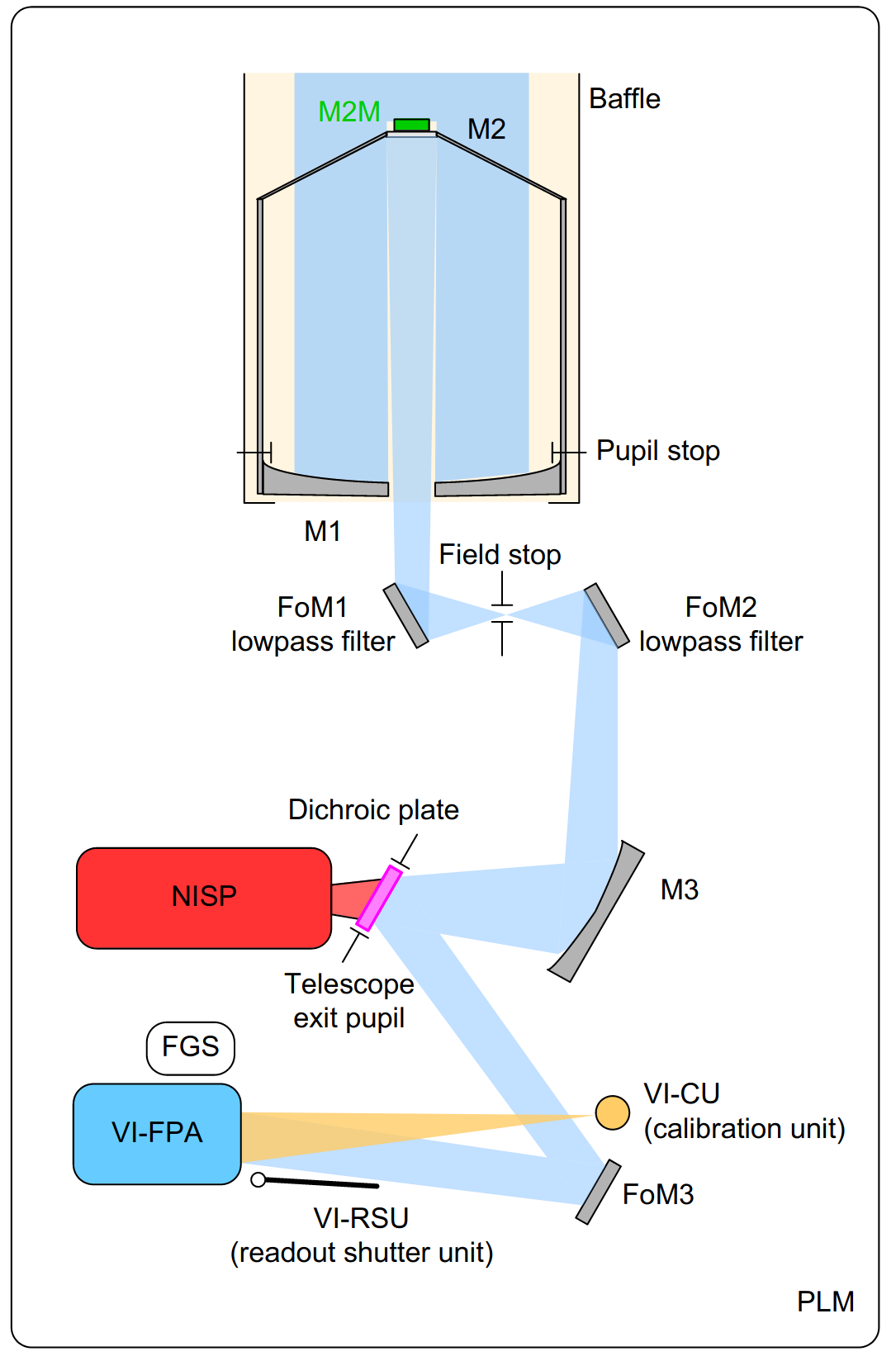
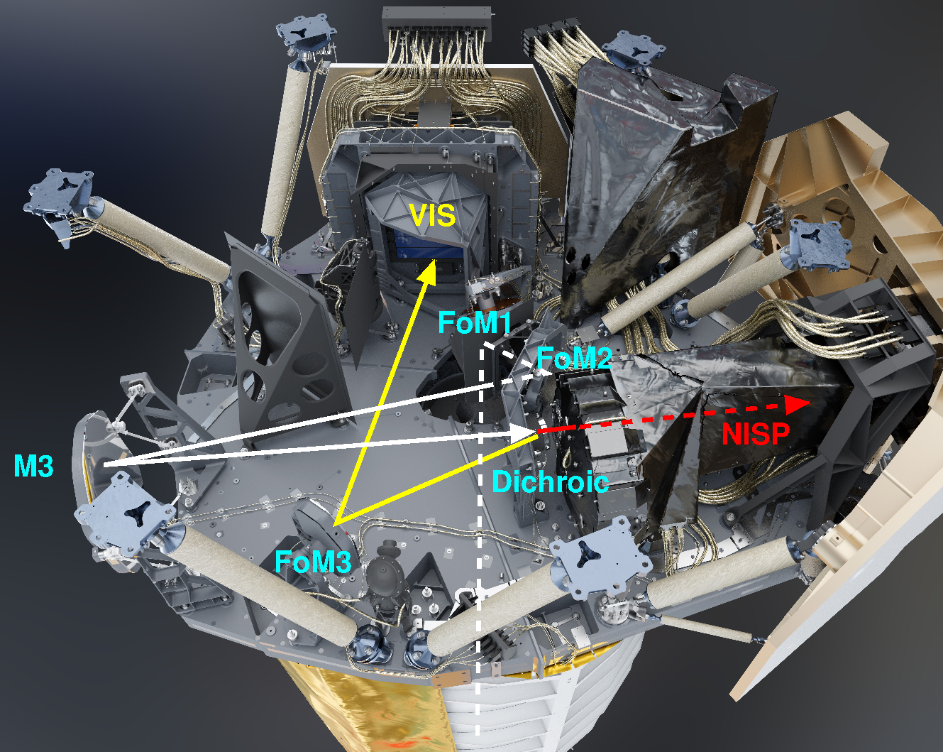
The PLM is divided into two cavities, separated by the baseplate. The front cavity includes the primary and secondary mirrors of the telescope, as well as the M2M and the associated support structure. This cavity is thermally insulated by a baffle that functions as a stray light shield and as a thermal radiator at the same time. Figure 7 shows an annotated overview of the instrument cavity, which includes the telescope folding mirrors, the tertiary mirror M3, the dichroic plate, the FGS, and the two instruments NISP and VIS – the latter with its separate FPA, filter and grism wheels, and calibration source components.
The PLM’s mechanical architecture is based on a common SiC baseplate that supports on one side M1 and M2, and on the other side the remaining optics and the two instruments. On the baseplate two planar low-pass coated folding mirrors, FoM1 and FoM2, fold the optical beam in the plane of the baseplate at the entrance of the instrument cavity between M2 and M3. A third, silver-coated folding mirror (FoM3) allows us to have the VIS instrument close to a radiator to efficiently remove the front-end electronics’ heat. The telescope is cooled down to its equilibrium temperature (M1 temperature around 126 K). This cold telescope offers high thermo-elastic stability, where the SiC’s coefficient of thermal expansion is reduced to 0.4 m-1 K-1, and provides a time-stable cold environment for the instruments. The baseplate temperature range of 130 K to 135 K is maintained constant during the mission to about 200 mK and to a few tens of millikelvin during the observations. The main drivers of the baseplate temperature are the attitude of the spacecraft and the local heat dissipation generated by the instrument units operational status.
3.2 Transfer and orbital maintenance
Euclid operates from a large-amplitude quasi-periodic halo orbit around L2, with a maximum Sun-Spacecraft-Earth angle of 35∘ and a period of about half a year. Euclid travelled on a so-called stable manifold towards its operational orbit, which did not require an orbit-injection manoeuvre. The Falcon-9 launch vehicle injected Euclid very accurately to this stable manifold. Of the three planned transfer correction manoeuvres (TCMs), only two were required. The first one was executed one day into the mission, providing a m s-1 to remove the launcher dispersion. The second TCM, three weeks after launch, delivered a correction of m s-1. Overall, a total of m s-1 was budgeted for all three TCMs, meaning that a considerable amount of propellant (about 43 kg) was saved for the scientific mission. However, it should be pointed out that the amount of hydrazine propellant is not a sizing parameter for the mission duration, which is limited by the amount of gaseous nitrogen used by the micro-propulsion system during the science observations.
The launch day and lift-off times were selected such that the resulting operational orbit is eclipse-free, without excursions into the Earth and Moon shadows. Such an excursion would result in a considerable thermal disturbance and also power limitation. The quasi-periodic halo orbit around L2 is dynamically unstable, that is the perturbations grow exponentially over time. Perturbations can be non-gravitational, from sources such as outgassing (Euclid Collaboration: Schirmer et al. 2023), imperfect thruster firings, leakage, variable solar radiation pressure, and offloading of wheel movements. Further perturbations occur in the time span from the on-ground processing to the actual correction manoeuvre; that is, the latter does not perfectly fit the true orbit anymore. The time constant of the exponential decay of a typical wide halo orbit is 22–23 days, and escape from the operational orbit occurs after approximately 90 days.
Station-keeping or orbital maintenance is achieved by thruster firings on a regular basis. A more frequent orbital maintenance keeps the exponentially growing perturbations better in check, meaning a smaller total velocity correction needs to be applied each year, saving propellant. Euclid requires slots of about 6 h per orbital maintenance, which would considerably reduce the time available for the survey if executed too frequently. The best compromise between propellant efficiency and survey efficiency for Euclid is by scheduling orbital maintenance at fixed intervals of 28 days (see also Euclid Collaboration: Scaramella et al. 2022). A total of 1000 orbital years were simulated by ESA, assuming various cases of residual acceleration from non-gravitational factors, spanning from m s-2 to m s-2. The yearly required with a 28-day maintenance schedule then ranges between 0.76 m s-1 and 7.00 m s-1, dependent on the assumed expected stochastic residual acceleration of the spacecraft. Other ESA missions at L2, such as Gaia, Planck, and Herschel, were found to be in this range of acceleration in their respective orbit-assessment analyses.
At the time of writing, only a few orbital maintenance manoeuvres were executed, insufficient to make a reliable estimate of the actual long-term fuel consumption. The current budgeting for Euclid is therefore necessarily conservative and for the worst case m s-1 per year assuming corrections every 28 days. These burns would last about 50 s on average and consume approximately 1 kg of hydrazine propellant. Euclid carries a total of 137.5 kg of hydrazine for transfer corrections into the L2 orbit, orbit maintenance for six years, and disposal into a heliocentric graveyard orbit (Racca et al. 2016). The latter is required by ESA’s space-debris mitigation code of conduct, and requires up to m s-1.
3.3 Pointing constraints and data downlink
The Euclid image quality requirements demand very precise pointing stability, while the survey requirements call for fast and accurate slews. The image quality requirements were translated into AOCS requirements on the relative and absolute pointing errors (RPE and APE, respectively) at the 99.7% confidence level. In science mode, the allowed RPE over a period of 700 seconds121212The longest Euclid science exposures are about 570 s (see Table 3). around the - and -axes of the spacecraft is 75 mas (milli-arcseconds), and around the -axis (roll angle). The allowed APE is around the - and -axes, and around the -axis.
An FGS with four charge-coupled device (CCD) sensors co-located within the focal plane of the telescope at the side of the VIS imager provides the fine attitude measurement based on a pair of operational CCDs. Cold-gas micro-propulsion thrusters with micro-Newton resolution provide the fine torque commands used to achieve the high-accuracy pointing. The gyro- and FGS-based attitude control corrects for low-frequency noise, ensuring that the RPE requirement is met. Three star tracker optical heads used in a 3:2 cold redundancy scheme provide the inertial attitude. The star trackers are mounted on the SVM and are thus subject to thermo-elastic deformation when large slews are executed. The FGS is also endowed with absolute pointing capabilities – based on a reference star catalogue – to comply with the APE requirement. This capability allows the autonomous cross-calibration of the star trackers and FGS so that the commanded target attitude is achieved for the subsequent observation. A high-performance gyroscope is included to propagate the FGS attitude between two measurements and during the temporary FGS outages, for example, when operating the VIS shutter (see Sect. 3.4 below).
Three or four reaction wheels execute the science mode slews, specifically field, dither, and large slews between different sky zones. Before the end of the slew manoeuvre, the wheels’ torques are commanded to zero and the wheels are left to brake on their own friction. Keeping the reaction wheels at rest during observations ensures noise-free science exposures by eliminating micro-vibrations and torque-noise effects.
Finally, to optimise the PSF (Sect. 7.6.4) and reduce its variability, thermal variations need to be minimised to avoid degrading the image quality as much as possible. This places restrictions on the spacecraft attitude and internal power dissipation variations that can be tolerated. To quantify these, an analysis of the full structural thermal optical performance (STOP) of the satellite was performed, where the impact of the spacecraft attitude variations on the PSF stability was studied (Anselmi et al., in prep.). This resulted in limiting the allowed range in Solar aspect angle (SAA) and alpha angle (AA). SAA is defined as the angle between the spacecraft’s -axis (telescope pointing direction; see Fig. 5) and the Sun vector (direction to the centre of the solar disk from the origin of the spacecraft reference frame). AA is defined as the angle between the Sun vector projected onto the – plane and the -axis, and it increases as the spacecraft rotates clockwise about its -axis. In addition to the range limitation, further minimisation of the field-to-field variation in these angles is desirable. The range of AA and SAA considered and its implication for the survey design are discussed in Sect. 4.1 and Sect. 5.4.
3.3.1 Data downlink
Euclid can use a 4-hour long daily telemetry communication period (DTCP) to downlink its science data and recorded telemetry, about 826 Gbit of compressed data per day, either to the Cebreros (Spain) or the Malargüe (Argentina) ground station. The science data are transmitted using the consultative committee for space data systems file delivery protocol (CFDP), which simplifies science operations and processing. This is the first time this protocol has been used from L2. The downlink is performed with Euclid’s steerable 70-cm diameter -band high-gain antenna (HGA). From Euclid’s perspective, the Earth traces approximately a wide ellipse on the sky every 6 months, with an opening angle of about 35∘ and the Sun near the centre. The beam width of the HGA is smaller than the apparent diameter of the Earth as seen from Euclid, about , meaning that the HGA’s position must be adjusted frequently. Adjustments are permitted during spacecraft slews only, so as not to disturb the pointing stability during an ongoing observation.
Within a DTCP window the HGA follows a ground station, accounting for Earth’s rotation for maximum antenna gain. The HGA is repositioned with every dither slew, that is 3 times per survey field or approximately every 20 minutes. Outside a DTCP window the HGA is repointed to the position where a ground station is expected to appear at the next DTCP. This happens every 72 min when slewing to the next survey field, but an actual antenna movement might not be required every time.
To simplify spacecraft operations, the DTCP windows are decoupled from the scientific observations, that is the HGA must be allowed to repoint at most every 50 minutes. This means that Euclid cannot stare at the same position on the sky for longer than 50 min. Both the Euclid survey and our calibration programme (Sect. 4.3) are designed to fit within this constraint, which will likely also apply to future mission extensions and potential mini-surveys during windows of unallocated time (Sect. 4.1.2).
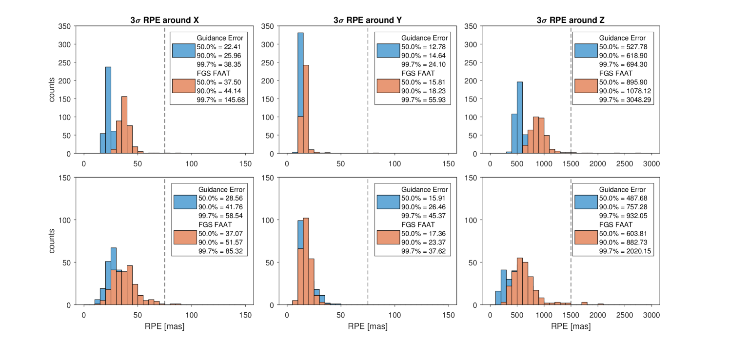
3.3.2 Pointing accuracy and stability
In-flight estimates of the absolute pointing error (APE) are larger than the requirements by a factor 2 or more: around the spacecraft’s -axis, around the -axis, and around the -axis, with the axes shown in Fig. 5. This is sufficient for survey purposes, but it also means that Euclid cannot place an object onto a specific pixel.
Similarly, the RPEs can be estimated from a range of orbital house-keeping parameters, providing slightly different results as they were intended for different purposes. We used the RPE contained in the AOCS ‘guidance error’ vector and the absolute quaternion produced by the FGS. In Fig. 9 we show our findings from an analysis of 360 VIS nominal science exposures and 243 VIS short science exposures taken from 5 to 9 December 2023, after an AOCS software update to improve the pointing performance. These results should be representative for the remainder of the survey.
Accordingly, for nominal exposures the RPE around the -axis is poorer than around the -axis, but still fully compliant if the guidance error vector is considered (38 mas at 99.7% confidence level), while it would exceed the requirement (75 mas) if the FGS absolute quaternion is considered. Around the -axis the requirements are fulfilled using both indicators. Around the -axis the situation is similar to the -axis and the requirement (1500 mas) is exceeded if the FGS absolute quaternion is considered. The RPE for short science exposures is somewhat different due to the larger fraction of the stabilisation time in the exposure. A full discussion of these results is beyond the scope of this paper. Concerning the PSF reconstruction, the FGS absolute quaternion should be used only for the - and -axes, while for the -axis the pointing derived from the FGS quaternion should be combined with the more accurate gyroscope vector.
The pointing stability during an exposure is about 35 mas or 1/3 of a VIS pixel around the - and -axes with 99.7% confidence. This is achieved by continuous operation of cold-gas thrusters to counter non-gravitational accelerations, mainly from solar radiation pressure but also from outgassing. In the magnitude range 10 to 19, Euclid’s FGS can find sufficient guide stars for the great majority of fields (99.9%) when the telescope is focused; exceptions are Euclid’s VIS wavefront-retrieval observations, where the telescope must be slightly defocused (Sect. 4.3.2).
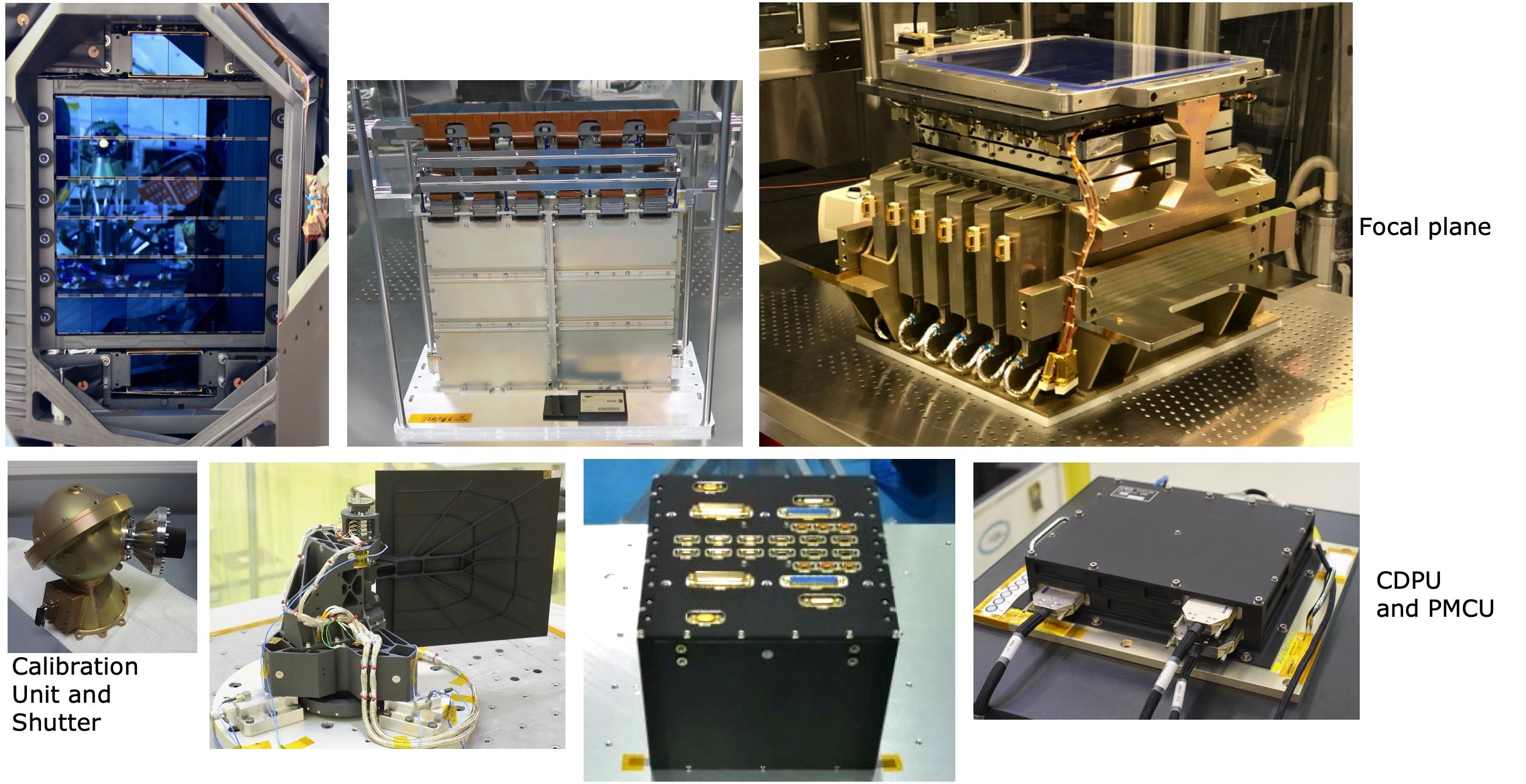
3.4 Visible instrument: VIS
To enable the weak gravitational lensing science discussed in Sect. 2.2, accurate shapes need to be measured for about 1.5 billion galaxies. This requires an instrument that can image large parts of the Universe with fine spatial resolution. Galaxies in the redshift range , which will be used to map dark matter, have typical angular diameters of and must be sampled with resolution or better. The Euclid instrument designed to meet these requirements, VIS, is a large-format imager with an FoV of 0.54 deg2 sampled at pixel-1, operating in a single red passband. The considerations driving the VIS design, and its development and initial performance, are described in detail in Euclid Collaboration: Cropper et al. (2024); a brief overview is provided here. A mosaic of the VIS subsystems is shown in Fig. 10.
The cosmological lensing signal is extracted from a statistical analysis of a large number of coarsely sampled faint galaxies. With sample sizes to achieve the precision targeted in Sect. 2.2, biases in the measurements become dominant. Obtaining meaningful results, therefore, depends critically on a deep understanding of the instrumental effects. VIS fits within a system of external optics, calibrations, and survey design, all of which have been highly and mutually optimised to meet the stringent performance required for weak gravitational lensing (Cropper et al. 2013). VIS is therefore designed to be maximally stable and able to be calibrated.
The VIS detectors are CCDs, which were chosen because of the detailed understanding gained from past missions on their behaviour and performance in the space environment, and their stability, which results from the signals passing through a limited number of readout nodes. In order to cover the large FoV, VIS has 36 CCD273-82 designed and manufactured by e2v (Endicott et al. 2012) to a custom Euclid specification (Short et al. 2014) in a array (see Fig. 11). Each CCD has pixels in four quadrants, so the VIS images comprise pixels. The pixels in the 144 separate quadrants are read out synchronously, to minimise noise, and digitised to 16-bit precision by 12 front-end electronics units. They are then passed to a control and data processing unit (CDPU; Di Giorgio et al. 2010, 2012; Galli et al. 2014), where the image is constructed and losslessly compressed, then sent to the spacecraft for downlink to Earth.
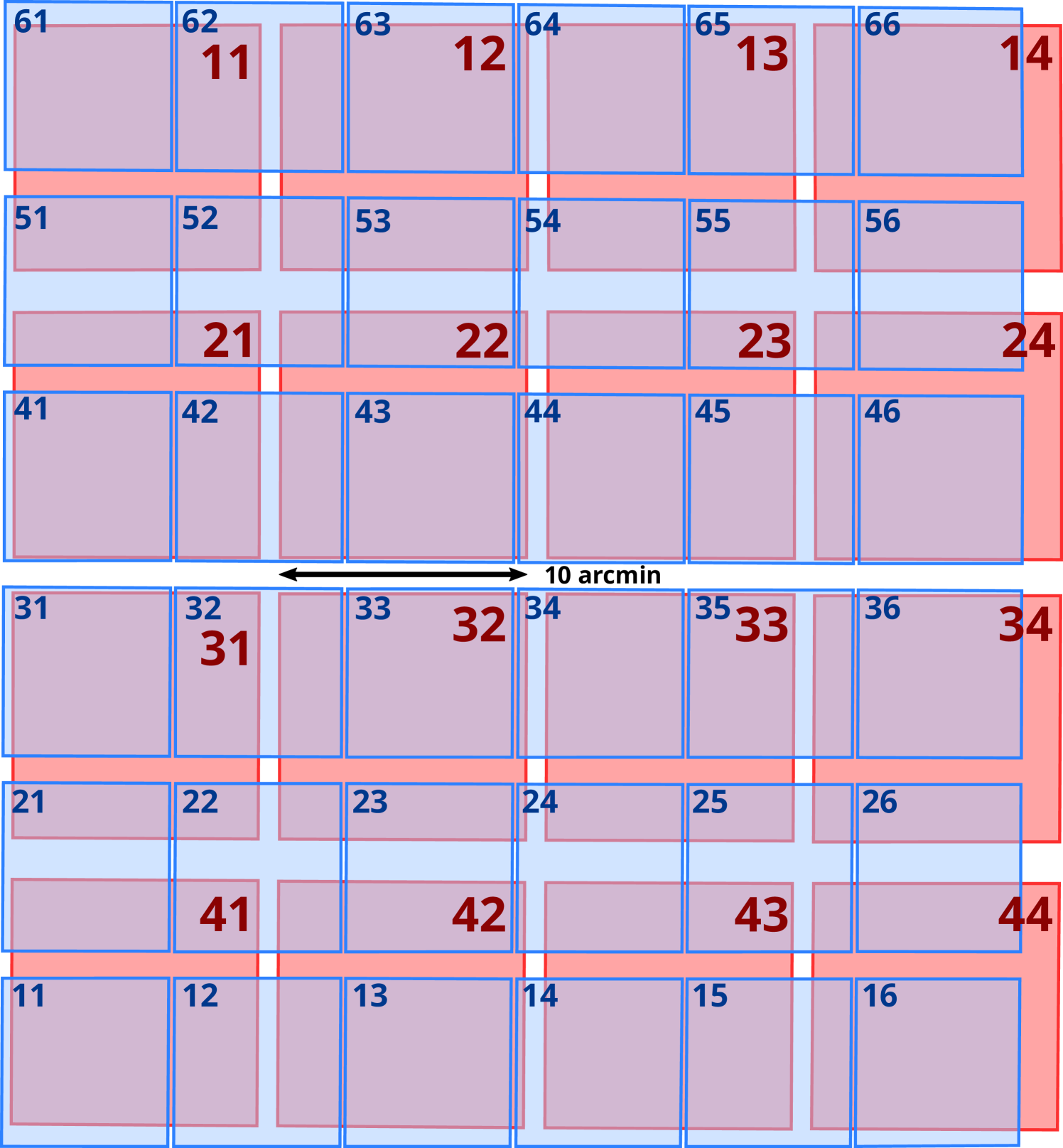
The CCDs are held in an SiC structure (Martignac et al. 2014) within the PLM at 153 K to minimise dark noise and optimise their performance in the presence of radiation damage (mainly by solar protons) to the Si-lattice within the devices. Although the pixel-to-pixel transfer of charge during readout of the image is very good, electrons can be temporarily trapped if they encounter a damaged site. When they escape, they can then be released into a charge packet of a later pixel. Hence galaxy shapes can be distorted because of missing charge in their pixels closer to the readout register or readout node, and spurious additional charge in pixels further from them. These distortions have a direct effect on the measured shape of a galaxy and are therefore of concern (e.g. Massey et al. 2014; Israel et al. 2015). A number of enhancements to minimise these effects were incorporated into the Euclid CCD273-82 design, including an enhanced capability to inject charge directly into the image area, even at low charge levels, to quantify the distortions from the traps. Its operational parameters were optimised for Euclid in an extensive characterisation campaign (Clarke et al. 2012; Prod’homme et al. 2014; Skottfelt et al. 2017b), with novel tri-level clocking schemes and the capability to shuffle charge repeatedly backwards and forwards – referred to as ‘trap pumping’ – to identify trap locations in both the image area and the readout register (Skottfelt et al. 2017a). Charge-injection and trap-pumping calibrations are run repeatedly throughout the survey (see Table 3).
Behind the SiC structure holding the 36 CCDs, 12 sets of readout electronics units (ROEs; Cropper et al. 2016; Szafraniec et al. 2016) set the operating conditions for the CCDs, clock them to read them out and digitise the pixel charge signal from the 144 CCD quadrants. They in turn, with their 12 power supplies, are combined in an aluminium structure (Martignac et al. 2014) that is interfaced to an external radiator to dissipate the heat from the ROEs. These operate at 270 K, so that thermal shields are used to minimise the parasitic heating of the CCDs held nearby in their SiC structure, nearly 120 K colder. These two halves comprise the FPA shown in Fig. 10. They are integrated on each side of a substantial SiC bracket on the PLM baseplate (see Fig. 7).
In order to maximise the stability of the VIS imaging, the instrument does not have a filter wheel; at the level required by Euclid this would not permit sufficiently repeatable image registration from exposure to exposure. The bandpass for the instrument is therefore set by the Euclid telescope, dichroic plate, the folding optics (Fig. 6), and the quantum efficiency (QE) of the CCDs, to be in the range 530–920 nm, optimised for the spectral energy distribution of the majority of galaxies. The wide band and high throughput (Fig. 12) provide a limiting sensitivity of ( point source), so that galaxies with a full width at half maximum (FWHM) of and are detected with in a 3 diameter aperture, sufficient for precise shape measurements. At the same time, however, the wide band complicates the shape measurement, because the PSF is chromatic. Although the entire VIS optical channel is in reflection, faint off-axis optical ghosts are created by the rear surface of the dichroic, and these must be masked in post-processing.
The CCDs are read out at 73 kHz to limit readout noise, and require a shutter (Genolet et al. 2016) to avoid image trailing from continuous illumination during readout. For reliability, the shutter is a single leaf with dimensions sufficient to cover the CCD array. It is momentum-compensated to a fine degree to minimise the disturbance to the Euclid pointing and hence the recorded PSF, which must be modelled to a high level of fidelity for accurate shape measurements. The shutter and a calibration unit for generating flat fields (Cropper et al. 2018) are driven by a power and mechanism control unit (PMCU; Renaud et al. 2018). This unit and the CDPU reside in the SVM, while the FPA with its electronics, the shutter, and the calibration unit reside in the PLM. The full complement of VIS units is shown in Fig. 10.
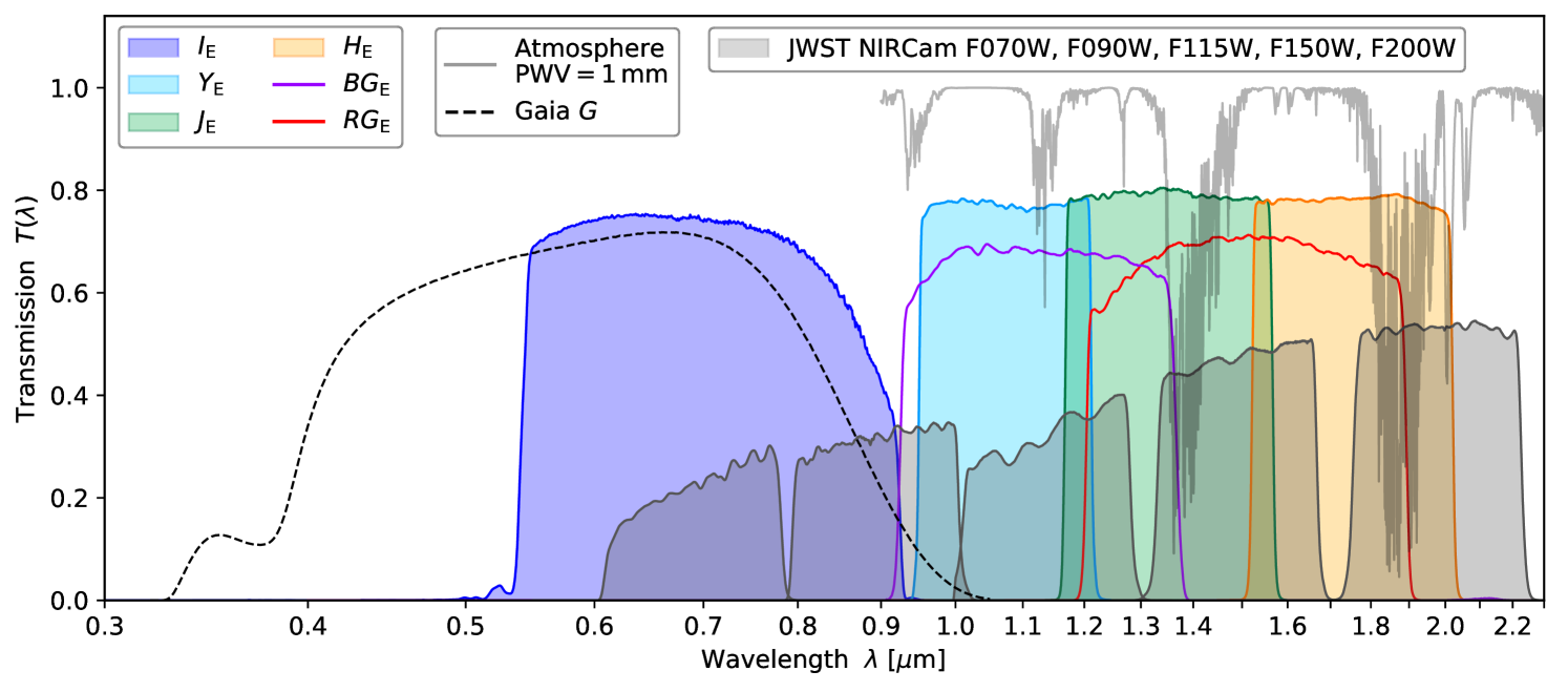
3.5 Near-Infrared Photometer and Spectrometer: NISP
The second instrument on board Euclid is the Near-Infrared Spectrometer and Photometer (NISP, Fig. 13), described in more depth in Maciaszek et al. (2022) and Euclid Collaboration: Jahnke et al. (2024). NISP provides multiband photometry and slitless grism spectroscopy in the wavelength range 920–2020 nm (Fig. 12), using the light transmitted by the dichroic beamsplitter.
3.5.1 Hardware overview
NISP has a common optics and detector system for its photometric and spectroscopic channels, with respective filters and grisms in two wheels.131313It is not permitted to use elements from both the filter and grism wheels at the same time, because both have some optical power. Hence, a simultaneous observation through both elements, for example to produce shorter spectra with smaller overlap fractions, results in strongly defocused images. A collimator lens provides for each individual source a nearly parallel beam through the filters and grisms. A subsequent camera-lens assembly, together with slight optical power on grisms and filters, focuses the beam in the detector plane. Details and consequences of this design, such as passband variations, are discussed in Euclid Collaboration: Schirmer et al. (2022).
The filter wheel includes a dark plate that can be used to block all light from the telescope, but not from the calibration lamp, for specific calibration purposes. The lamp uses five nearly monochromatic light-emitting diodes (LEDs) whose wavelengths span the NISP wavelength range to support a wide spectrum of calibrations (Sects. 4.3.1, 4.3.3 and 4.3).
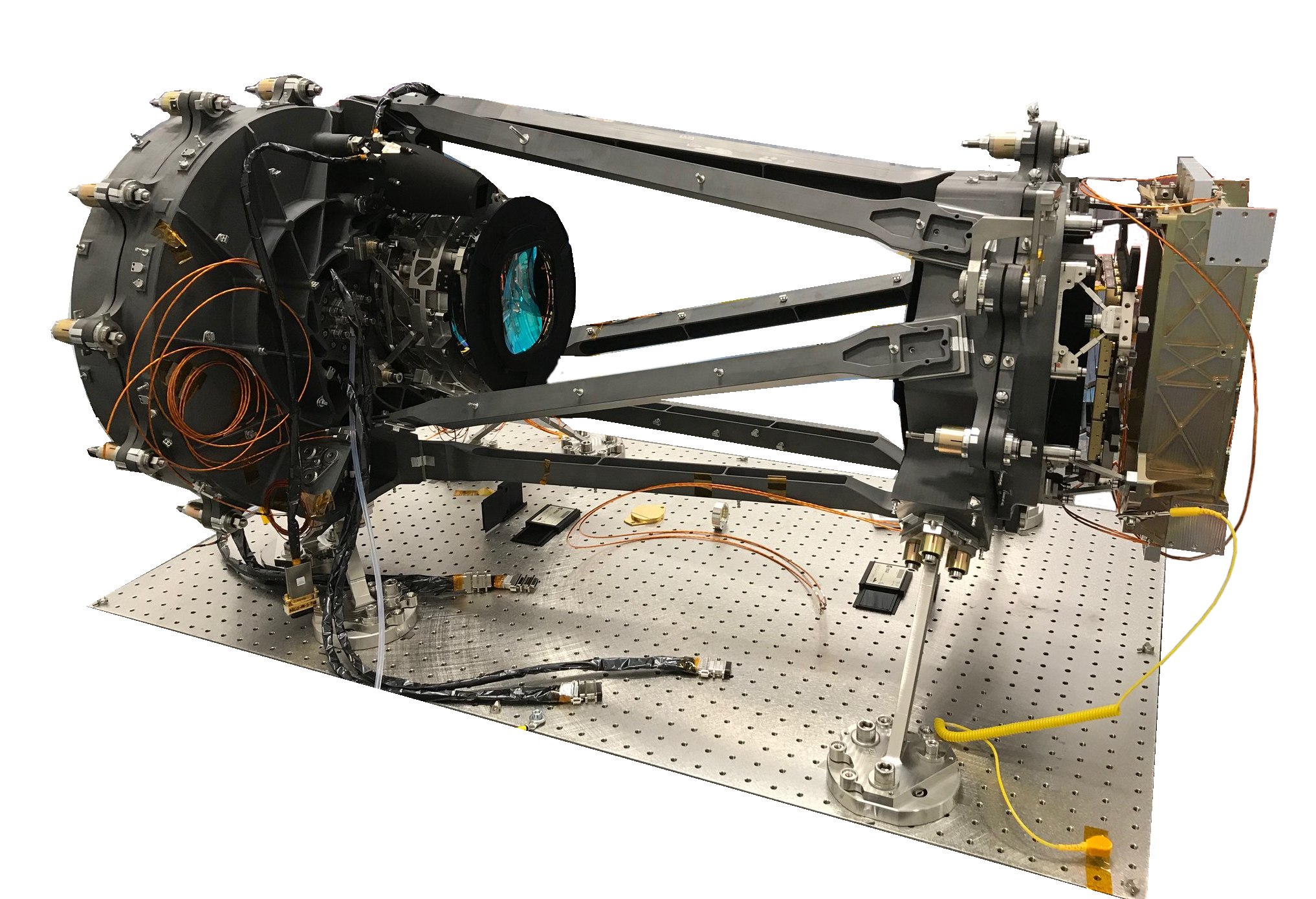
The FPA consists of a grid of Teledyne Hawaii-2RG (H2RG) detectors with pixels. A four-pixel wide border along the detector edges is not light-sensitive, providing baseline reference pixels for detector monitoring. With a plate scale of pixel-1 and including detector gaps, the NISP FoV covers a nearly square-shaped 0.57 deg2 (see Fig. 11).
The 16 H2RGs are operated at K to optimise detector behaviour, while the main optics is kept at 130–132 K. Parallel readout occurs in 32 channels per detector using a multi-accumulate (MACC) scheme, with NISP continuously read at a nominal rate of 1.45408 s per frame. For science and calibration exposures, a group of each 16 successive frames is read non-destructively and averaged by the on-board data-processing unit (DPU). Between these groups the exposure just continues and photons are collected, but a number of frames are not read (so-called ‘drops’), either since they would not add up to another group of 16, or due to running into NISP storage limits. At the end, the count rate in each pixel is determined with a linear slope fit to the group values using an iterative algorithm (Kubik et al. 2016). Standard photometry and spectroscopy exposures for the Euclid Wide and Deep Surveys (Sect. 4) use four and 15 groups with 16 frames each, and a number of four and 11 dropped frames, respectively; we refer to these modes as MACC(4,16,4) and MACC(15,16,11). The effective integration times for the photo- and spectro-exposures are 87.2 s and 549.6 s respectively, while the actual exposure durations are 110.5 s and 572.9 s. The latter times are relevant for the survey planning (Sect. 4), while the former determine the depth of the science data.
NISP uses cold readout electronics at the focal plane, and warm electronics operating at K located in the SVM. The warm electronics contain both the commanding computer and the DPU. The latter performs the baseline subtraction using reference pixels, the MACC slope fit, and the data compression. For images the compressed slope-fit image is downlinked together with a 1-bit quality image that encodes whether the slope-fit lies above a certain threshold. For dispersed spectra images the full information is downlinked in an 8-bit quality image. NISP has full redundancy in its warm electronics and calibration-source LEDs, as well as the power supply to drive the filter and grism wheels.
3.5.2 Near-infrared imaging
The NISP photometric channel (NISP-P) offers three passbands (949.6–1212.3 nm), (1167.6–1567.0 nm), and (1521.5–2021.4 nm), displayed in Fig. 12. The wavelengths refer to the 50% peak-transmission points near the centre of the FoV and are accurate to 0.8 nm. Passband variations within the FoV are characterised to nm. The near-rectangular passband flanks are entirely defined by the 130-mm diameter filters, which carry up to 200 interference coating layers distributed over both filter sides (Euclid Collaboration: Jahnke et al. 2024). The total in-band spectral response, including detectors, is close to 80%. Out-of-band blocking is 10-4 or better within 900–2100 nm, and to outside this range. These excellent blocking capabilities are jointly achieved by the filters, all other coated optical surfaces in the NISP optical path, and the detectors (Fig. 8). Out-of-band contamination is at most 2.0 mmag for sources with extreme SEDs, and more typically 0.2 mmag. More details about this and the NISP photometric system in general are presented in Euclid Collaboration: Schirmer et al. (2022).
The designed point-source depth of NISP-P for the wide survey is 24.0 AB mag, which we exceed by approximately 0.4 mag (Sect. 5). The plate scale of pixel-1 considerably undersamples the NISP PSF that has a typical FWHM of 1.10, 1.17, and 1.19 pixel in , , and when fitting a Moffat profile (see also Bernstein 2002). The measured PSF size is fully compatible with the on-ground characterisation of the NISP optics (Grupp et al. 2014). Details are given in Sect. 5.
3.5.3 Near-infrared spectroscopy
The NISP spectroscopic channel (NISP-S) enables the simultaneous acquisition of slitless spectra for thousands of objects across the FoV with uniform quality. The grism wheel houses four different grisms of 140-mm diameter each. The grisms are dispersion gratings combined with a prism whose base is – just like the filters – slightly curved for optimal focus. Dielectric coatings improve out-of-band blocking (Euclid Collaboration: Jahnke et al. 2024). The total spectral response including all optical surfaces and detectors is shown in Fig. 12.
For the spectroscopic observations of the EWS (Sect. 4.1) NISP-S uses three red grisms covering the same passband (1206–1892 nm; 50% peak transmission wavelengths), allowing the detection of H emitters in the range –. These grisms have different dispersion directions of , , and with respect to the detector columns. By combining the dispersed slitless images of the same field, overlapping spectra from multiple sources can be disentangled (‘decontaminated’) and clean spectra extracted. The red grisms have a dispersion of nm pixel-1 and a resolving power of for a source with diameter. The mission requirement is to achieve a redshift accuracy of . During the ground tests in 2020 it was discovered that the grism does not conform to the specifications and cannot be used for the survey. To achieve spectral decontamination, we use the other two red grisms with additional rotational offsets of the grism wheel, providing a total of four different dispersion directions (for details see Euclid Collaboration: Scaramella et al. 2022). The rotated positions vignette one edge of the detector array by up to 10%, which is accounted for by our calibration, while still meeting the overall image quality requirements.
The designed target sensitivity for the wide survey is a detection for an emission line with flux at 1600 nm (such as redshifted H), for a source with diameter. The in-flight performance was not yet available at the time of writing; however, given the excellent spectral image quality and the fact that NISP-P exceeds its designed depth by 0.4 mag, we are confident that NISP-S also meets its sensitivity requirement.
NISP-S also has a blue grism covering 926–1366 nm, extending the lower H redshift limit to . The blue grism has a resolution of 1.239 nm pixel-1 and a resolving power of . The blue grism is solely used for observations of the Euclid Deep and Auxiliary fields (Sect. 4.2). Its main purpose is to provide a large reference sample of galaxies with 99% redshift completeness and 99% purity required to characterise the typical Euclid galaxy population, while maximising the legacy value of these fields (Sect. 10).
4 Survey planning
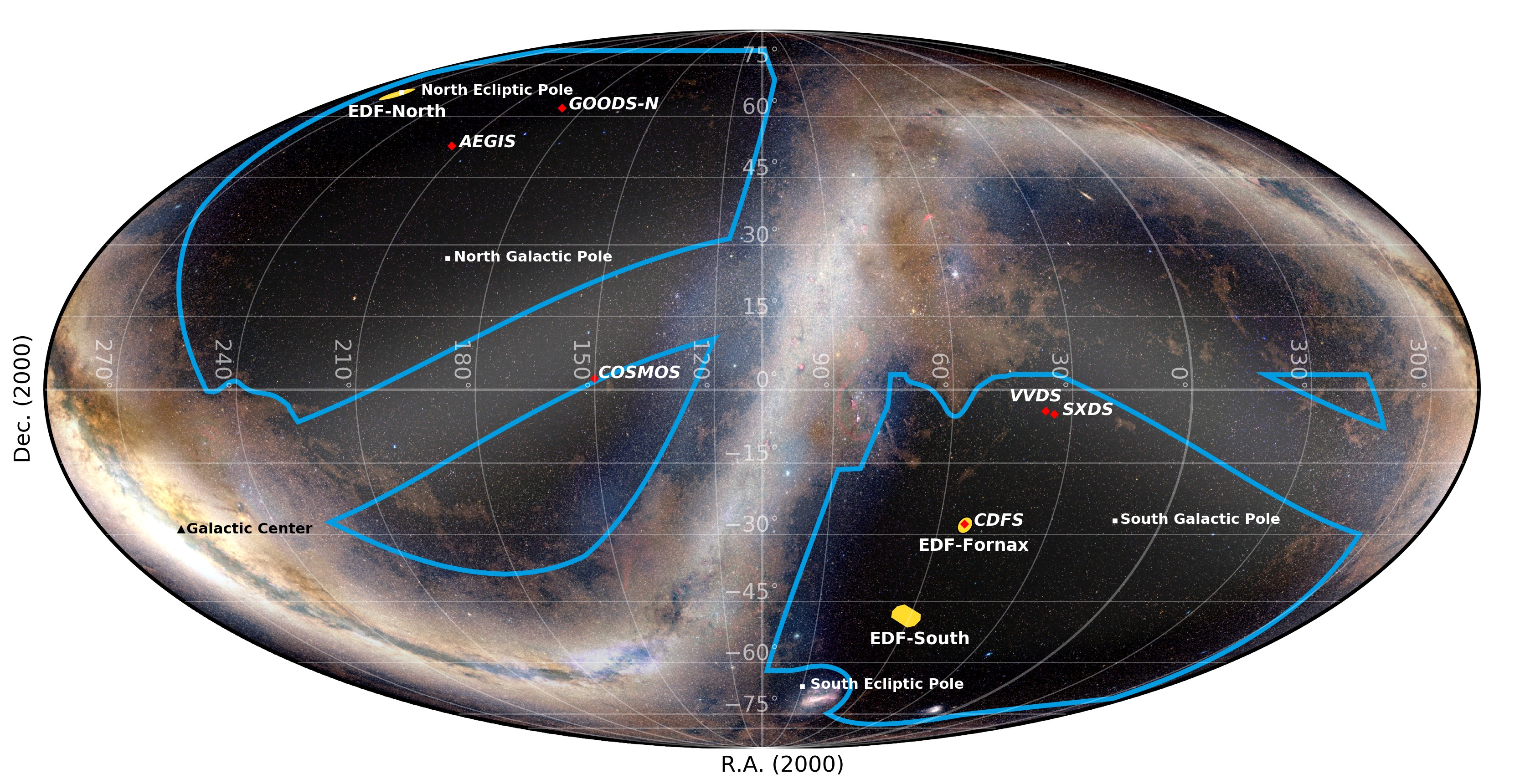
To achieve its primary cosmology objectives, Euclid aims to observe a sample of 1.5 billion galaxies for the 3×2pt analysis, and measure 35 million redshifts for the analysis of the spectroscopic clustering signal. To do so, it needs to cover about 14 000 deg2 of extragalactic sky with low zodiacal background and low Galactic extinction over a period of about six years. In Sect. 4.1 we summarise the design of the EWS. As discussed in Sect. 4.2, these data are complemented by deeper observations over several tens of square degrees, while the performance of the instruments is studied using extensive calibration observations, which are described in Sect. 4.3. Finally, the supporting ground-based observations are summarised in Sect. 4.4 (photometry) and Sect. 4.5 (spectroscopy).
| VIS | |
| 4 -band nominal exposures | 566 s each |
| 2 -band short exposures | 95 s each |
| Bias | 2 per day |
| Dark | 4 per day |
| Flat | 6 per day |
| Trap pumping | 6 per day |
| Charge injection | 8 per day |
| NISP | |
| 4 red-grism spectro exposures | 574 s each |
| 4 -band exposures | 112 s each |
| 4 -band exposures | 112 s each |
| 4 -band exposures | 112 s each |
| 1 Dark | 112 s |
4.1 Euclid Wide Survey
Euclid Collaboration: Scaramella et al. (2022) provides a detailed description of the reference EWS. Here, we summarise its characteristics and highlight the main modifications that were implemented prior to launch. The target area has minimal contamination from the Galaxy, Solar System objects, and the zodiacal background, that is the diffuse sunlight scattered by interplanetary dust in the ecliptic plane. The intersection of the avoided regions around the Galactic and ecliptic planes leaves four separate dark areas on the sky for the EWS, which we refer to as the RoI of Euclid, indicated by the blue lines in Fig. 14. These areas are adjusted in size to maximise the overlap with the ground-based surveys providing complementary data (Sect. 4.4) needed for PSF modelling and photometric redshift estimation. In the latest pre-launch configuration, the EWS covers 14 816 deg2 of the darkest extragalactic sky, of which 137 deg2 are lost due to about 800 bright stars with a magnitude in any Euclid band. As a result, the effective sky area is 14 679 deg2.
As detailed in Laureijs et al. (2011), for the VIS imaging we require a for extended sources with a diameter of times the FWHM of the PSF at AB mag. For NISP, we must reach a for point sources with in all three NISP bands, and for an H line flux of at a redshifted wavelength of 1.6 in the spectra. We show in Sect. 5 that these depth requirements are met with considerable margin. However, as discussed in more detail in Sect. 5.4, unacceptable levels of stray light were observed for certain spacecraft attitude angles. Avoiding these orientations is possible, but it also means that the effective sky area of 14 679 deg2 for the EWS can no longer be met within the nominal mission duration.
The ROS is the building block of the survey, comprising four dithered exposures that form an ‘S’-like pattern; the three dithers that follow the first exposure are in ecliptic coordinates151515In this paper we use the Greek letter for the Galactic longitude to avoid confusion with wavelength . , and , respectively. Table 3 lists the data collected during a typical sequence for a given survey field. In addition to the science data, various calibration exposures are obtained. The ROS lasts 70.2 min, followed by a slew to the next adjacent survey field. Such field slews take 2–4 minutes. Occasionally, large slews are required to begin a new survey patch on the sky, or to perform specific calibration observations. These last between 7 and 33 minutes, and their occurrence is kept to a minimum. Hence, about 20 fields are observed per day.
The EWS itself consists of about 27 500 fields, each of which is observed once with the ROS. Including Euclid Deep Survey (EDS) and calibration observations, the total survey comprises around 49 000 fields.
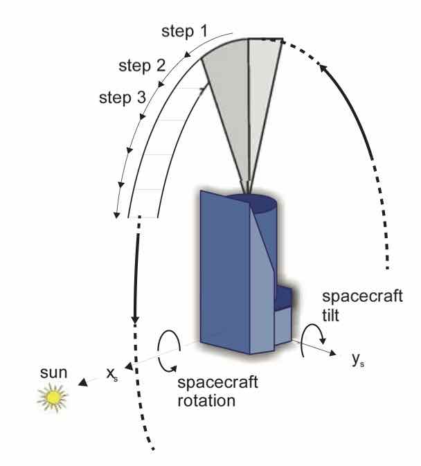
4.1.1 Principal survey strategy
Here, we describe the fundamental principles of the survey design. Significant modifications with respect to the pre-launch strategy are introduced in Sect. 5.5, because of the need to avoid stray light that was discovered post-launch at certain spacecraft attitude angles.
For ecliptic latitudes the EWS tessellates the RoI with non-overlapping identical tiles aligned with the ecliptic meridians, distributed along parallels of latitude. This configuration minimises overlaps and maximises survey efficiency. A tile is a FoV placed aligned with the meridian passing through its centre. The size of the tiles is computed from the intersection of the VIS and NISP FoVs. The tiles are observed in a step-and-stare mode by placing the larger Euclid common FoV (Fig. 11) on the four dithered positions of each tile. The minimum average overlap between neighbouring fields is 2.2% in area, occurring when all fields are aligned with their respective tiles. For the polar caps at a different tiling strategy was chosen to avoid excessive overlaps due to the converging meridians; details are given in Euclid Collaboration: Scaramella et al. (2022).
The basic position of the Euclid spacecraft has its sunshield facing towards the Sun, with the telescope pointing towards the north ecliptic pole (NEP). From this position Euclid can rotate freely around the Sun–spacecraft axis, keeping the sunshield orthogonal towards the direction to the Sun, so that it can point to any field on the transit ecliptic meridian, away from the Sun’s longitude (Fig. 15). The natural observing mode is to step-and-stare along the transit meridian, effectively sweeping the sky with transit meridians, at an approximate rate of per day, as Euclid progresses on its yearly orbit. The full circle defined by a transit meridian is divided in the ‘leading side’, the half-circle pointing in the direction of the spacecraft orbit, and the ‘trailing side’, the opposite half-circle. The two half-circles meet at the ecliptic poles. When observing in the trailing side the FoV is rotated in the sky.
The EWS is frequently halted to observe calibration fields at specific cadences. Moreover, as discussed in Sect. 3.2, all observations must stop every 4 weeks for orbital maintenance. During the interruption, the transit meridian moves and in order for the EWS to continue from the same point the spacecraft needs to tilt from its natural position (Fig. 15). In the latest pre-launch configuration, Euclid was allowed to point away from the transit meridian by tilting up to towards the Sun and up to away from the Sun, maximising thermo-optical stability; that is, the SAA range was restricted to .
If the interruption is too long, the last observed point of the EWS may no longer be visible with the allowed SAA range and can only be observed up to 6 months later, when the antipodal meridian is in transit.
Tilting from the transit meridian to another circle misaligns the FoV on the sky with respect to the orientation of the tessellation tiles. A rotation around the -axis (a change of AA; see Fig. 5) realigns the field with the tile. In the latest pre-launch configuration, the AA range was restricted to for thermal considerations. The limitations on the range of the two solar angles, SAA and AA, together with the need to keep the fields aligned (the ‘tessellation constraint’), defines the ‘window of visibility’ (Fig. 16). The window of visibility shows the span in longitude that Euclid can reach away from transit, and it is a function of ecliptic latitude . At low latitudes, where tilted observations do not introduce a misalignment of the FoVs, the longitude span is identical to the SAA range. Since the misalignment for a given tilt increases with latitude, the limited AA range available to align the FoVs drives the longitude span at high latitudes. Hence the window of visibility broadens towards the ecliptic equator. We note that without the tessellation constraint the ecliptic poles would have perennial visibility, and the window of visibility would broaden towards high latitudes, with the AA range playing no role in its definition. The longitude span is also directly related to how long a tile in the sky remains visible around transit.
Tiles are observed in sequences called ‘patches’, usually covering a latitude-longitude rectangle of the RoI. The viability in scheduling a patch is closely related to the window of visibility. Tiles must be visible at all latitudes of the tessellated RoI (). A reduced SAA range restricted to is used in practice to decrease the asymmetry of the window of visibility between high and low latitudes. Tiles must also be visible for a reasonable span of time; a longer visibility promotes wider patches.
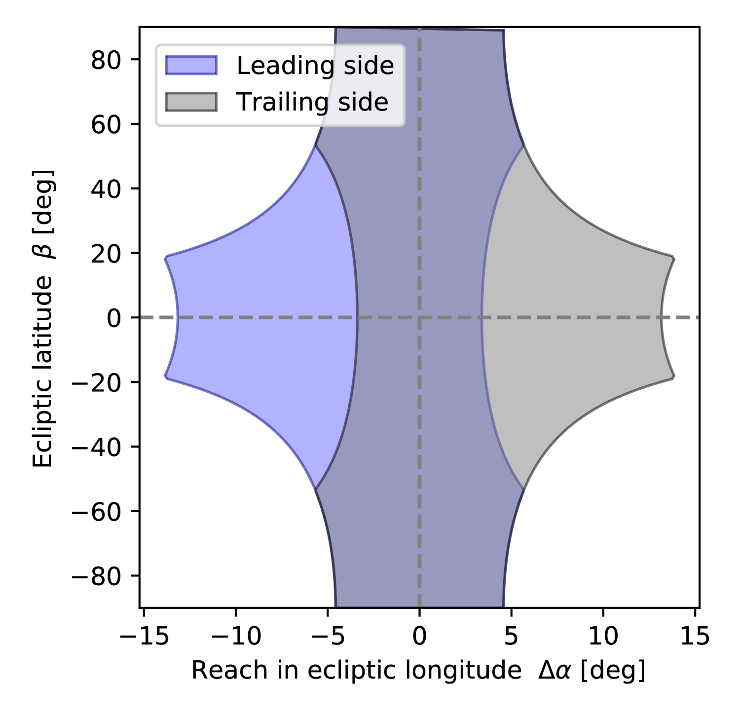
4.1.2 Unallocated time
The EWS is built by tiling patches layer by layer, starting from the poles, where the zodiacal background is lower, towards the ecliptic. The progression of the EWS also aims to observe the areas with complementary ground-based data as early as possible (Sect. 4.4). On the other hand, EWS observations must be scheduled continuously while the transit meridian scans the sky. However, longitude-wise, the area of the RoI is not uniform. At some point, the RoI area is exhausted where the Galactic plane intersects the ecliptic plane, and no EWS fields are available anymore for scheduling. This creates periods of unallocated time, all during the second half of the mission, that will then reappear regularly with a 6-month cadence, growing in duration. In the latest pre-launch configuration the unallocated time amounts to 9% of total time during routine operations (Fig. 17).
The periods of unallocated time will be used for different purposes. Foremost, they offer an opportunity for thermal decontamination of the PLM (Sect. 5.1), and to recover survey areas that were lost for example due to intermittent hardware problems, data-transmission losses, and severe space-weather events. Any remaining unallocated time not used for primary Euclid purposes could become available for targeted observations with the ROS, or for mini-surveys, possibly outside the RoI. Such opportunities, if any, will be developed and communicated in due time.
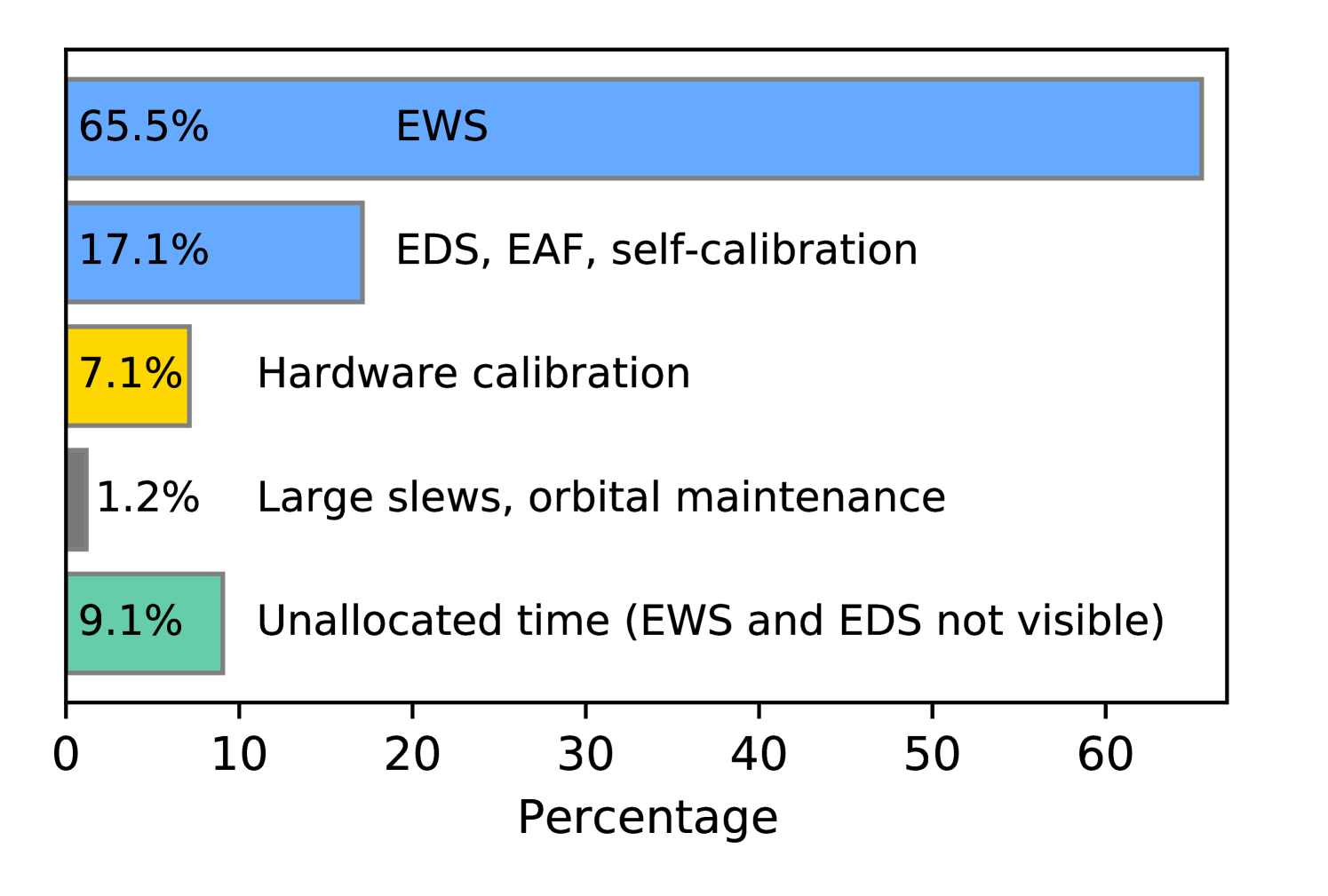
4.2 Euclid Deep Survey
The need to calibrate and monitor the telescope, cameras and electronics requires repeated visits of specific fields that will accumulate substantial depth over time. We also need to characterise the typical EWS source population and systematic effects, requiring deep data over a large area. In this section we present the motivation and characteristics of these data.
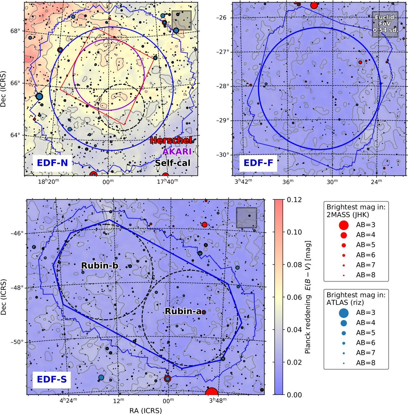
4.2.1 Euclid Deep Fields
About 12% of Euclid’s on-sky observations are spent on the EDS, for which we target a six-fold increase in S/N compared to the EWS, or a gain in depth of about 2 magnitudes. The primary purpose of the EDS is an accurate characterisation of the typical EWS galaxy population, that is a 99% complete and 99% pure spectroscopic sample of at least 120 000 galaxies, as well as accurate morphologies of galaxies to calibrate systematics in the weak-lensing shape measurement. The EDS also enables numerous legacy purposes, from primeval galaxies, galaxy and active galactic nucleus (AGN) evolution, and discovery of supernovae, to the structure of our Galaxy. It will uncover numerous targets for follow-up observations, and greatly extends the scientific scope of the mission beyond its core cosmology goals (Sect. 10).
Depending on the zodiacal background, at least 40 repetitions of the ROS are required to reach the desired EDS depth. Unlike the EWS, the EDS includes blue-grism observations with an exposure-time ratio of 5:3 for the blue relative to the red grism. The EDS comprises the Euclid Deep Field North (EDF-N), the Euclid Deep Field South (EDF-S), and the Euclid Deep Field Fornax (EDF-F). Figure 18 shows the layout of the three fields, which cover a total area of 53 deg2. The EDF-N is a 20 deg2 circular field located at the northern ecliptic pole. The EDF-F is a 10 deg2 circular field including the Chandra Deep Field South (CDFS), which has numerous ground- and space-based ancillary observations. Lastly, the EDF-S is a 23 deg2 field with an extended shape that encompasses two adjacent LSST deep-drilling fields.
4.2.2 Euclid Auxiliary Fields
The EDS is complemented by the EAFs. These fields are used for the calibration of photometric redshifts (Sect. 7.6.1) and to quantify the impact of colour gradients within galaxies on shape measurement in the presence of a chromatic PSF (e.g. Semboloni et al. 2013a). The EAFs include the COSMOS (Scoville et al. 2007), AEGIS (Davis et al. 2007), SXDS (Furusawa et al. 2008), VVDS (Le Fèvre et al. 2005), CDFS (Giacconi et al. 2001), and GOODS-North Giavalisco et al. (2004) fields (Table 4), which have been extensively observed by ground- and space-based telescopes. The CDFS is included in the EDF-F area, but observed independently for scheduling and technical reasons. The fields are observed up to 4–5 times the depth of the EWS.
4.2.3 Euclid self-calibration field and Ultra-Deep Field
The Euclid self-calibration field also belongs to the EAFs, but we discuss it separately here because of its technical significance. This field was chosen because of its location within Euclid’s northern continuous viewing zone that reaches up to from the NEP. This LoS offers a good stellar density for calibration and system-monitoring purposes, and at the same time gives a view of the extragalactic sky with acceptable reddening (see also Fig. 28). The LoS towards the South Ecliptic Pole (SEP) is less favourable due to obstruction by the outskirts of the Large Magellanic Cloud.
The self-calibration field fits in a radius of (Fig. 18), is located within the EDF-N area, and is observed on a monthly basis. We expect to exceed the typical wide-survey exposure time by a factor of 165 after 6 years, resulting in estimated point-source depths of 29.4 AB mag in , and 27.7 AB mag in , , and , that is about 3.2 mag deeper than the EWS. The central part ( radius) serves as a backup pointing to avoid idling during non-standard operations and maintenance. Thus the self-calibration field will eventually become the Euclid Ultra-Deep Field (EUDF). The final depth of the central part is not yet known, given that it will be observed an unknown number of times as a backup field.
| Field | RA | Dec | Area | Depth |
|---|---|---|---|---|
| Self-calibration | 268.813 | +65.29 | 2.5 deg2 | |
| AEGIS | 214.827 | +52.82 | 1.0 deg2 | |
| GOODS-North | 189.250 | +62.25 | 0.5 deg2 | |
| COSMOS | 150.119 | +02.21 | 2.0 deg2 | |
| VVDS-Deep | 36.500 | 04.50 | 0.5 deg2 | |
| CDFS | 53.117 | 27.81 | 0.5 deg2 | |
| SXDS | 34.500 | 05.00 | 2.0 deg2 |
4.3 Calibration observations
Euclid has tight calibration requirements. The VIS, NISP-P, and NISP-S data must meet respective relative photometric accuracy levels of 1.0, 1.5, and 0.7% over the full survey area and a 6-year mission duration. These requirements enable, respectively, a uniform photometric reference for the ground-based photometry (Sect. 4.4), accurate photo- measurements (Sect. 7.6.1), and a stable selection function for galaxy clustering (Sect. 7.7.1). To ensure a sufficiently unbiased weak lensing signal, the uncertainty in the estimate of the ellipticity of the VIS PSF model must be less than per ellipticity component, while the relative uncertainty in the area of the model PSF, quantified by its quadrupole moments, must be better than (Cropper et al. 2013).
We designed a rigorous calibration programme to monitor the in-flight performance and to counter the effects of space weathering and molecular outgassing (Euclid Collaboration: Schirmer et al. 2023) at any time in the survey. In addition, the galaxy population that Euclid observes must be characterised in specific fields. Hence our in-flight calibration activities fall into the following three groups.
4.3.1 Performance verification phase
Commissioning was followed by a 3-month long period for the performance-verification (PV) phase. During this time most system calibrations and characterisations for zero-gravity conditions and in-flight temperatures were updated. Not everything, however, could be repeated in-flight, such as measurements of the absolute QE. A total of 35 observing blocks were executed, the majority of which were based on specialised commanding sequences that were extensively tested on the ground. Whenever possible, on-sky calibrations were taken with the ROS, our fundamental survey building block, because it has been well tested and means that the calibration data were taken in the same way as the survey data, sometimes at the expense of increased overheads. Some initial results are highlighted in Sect. 5.
Each calibration block provides data for several calibration products that inform our error budgets. For NISP we have 12 common calibration products that serve NISP-P and NISP-S, such as: baseline map; brighter-fatter effect (Plazas et al. 2018; Hirata & Choi 2019); electronic crosstalk; dark current; interpixel capacitance (Le Graët et al. 2022); lamp flats; nonlinearity; reciprocity failure (count-rate nonlinearity; Biesiadzinski et al. 2011); and charge persistence.
Eight calibration products are for NISP-P, including absolute flux calibration, illumination correction, detector and optical distortions, ghost images, and the PSF model. NISP-S comprises eleven calibration products, including a complex calibration chain from astrometric positions on sky to individual wavelengths in the dispersed images, based among other things on observations of the compact planetary nebula SMC-SMP-20 (Euclid Collaboration: Paterson et al. 2023) in the Small Magellanic Cloud. For VIS we have a total of 24 calibration products, the majority of which cover electronic and detector properties such as bias, dark, brighter-fatter effect (Antilogus et al. 2014), nonlinearity, crosstalk, charge-transfer inefficiency (CTI; Israel et al. 2015), extended pixel-edge response (CTI-EPER; Robberto 2007), and more. The remainder comprises optical aspects such as the shutter map, illumination correction, stray light levels, lamp flats, and absolute flux calibration. Other PV activities focused on the telescope’s thermal response to solar attitude changes and instrument activities, molecular outgassing, and survey characterisations such as depth, sensitivity, scattered light, and zodiacal background.
4.3.2 Phase diversity calibration campaign
Euclid’s optics, telescope structure, and baseplate are constructed of SiC that is known for its low thermal expansion coefficient, high thermal conductivity, strength, and stiffness (Sect. 3.1.2). Euclid orbits L2 in a thermally stable environment (Sect. 3.2). Yet, at the level of our requirements, Euclid’s PSF is sensitive to spacecraft attitude changes well below , causing an initial thermal imbalance and a subsequent heat flow that affects different telescope parts at different times. The survey is therefore designed to minimise attitude changes while stepping from one survey tile to the next (Euclid Collaboration: Scaramella et al. 2022).
To ensure that an accurate PSF model (Sect. 7.6.4) can be derived for all observations in the presence of thermal variations, we must know the wavefront errors that may occur during the survey. Owing in part to the broad VIS passband, the wavefront errors cannot be retrieved from in-focus observations alone. We therefore employ a combination of in- and out-of-focus observations of stellar fields (see e.g. Wong et al. 2021). At the centre of this phase diversity calibration are four fields that are observed intra-focal, extra-focal, and in-focus; one of these fields has a high LoS polarisation. Six additional fields are observed in-focus only. All fields have known SEDs from Gaia and dedicated ground-based observations, and are also observed with NISP to improve the star-galaxy separation for compact sources.
For each field a different stable thermal state of the PLM is prepared prior to the observations, by maintaining the telescope for about seven days at a given solar attitude. Calibration and scientific filler programmes are run during the thermal stabilisation periods. About 60 days are required after the PV phase to retrieve the data for the PSF model. Routine survey operations began afterwards, in February 2024.
4.3.3 Routine phase
The three deep fields (Sect. 4.2.1) will yield at least 200 000 galaxies with a S/N 6 times that of the EWS. This provides improved morphological information that will aid the calibration of the weak lensing signal (Hoekstra et al. 2017, 2021). Blue-grism exposures are needed to provide a spectroscopic subsample of at least 120 000 galaxies with 99% redshift purity and 99% completeness for galaxy-clustering purposes, and to characterise the typical EWS galaxy population.
Euclid also observes the EAFs (Sect. 4.2.2 and Table 4), for which multiwavelength data by Hubble Space Telescope (HST) are available. The spatially resolved colour information from HST is needed to quantify shape-measurement biases introduced by colour gradients within a galaxy; these biases are inevitable for a diffraction-limited PSF in Euclid’s wide -band (Voigt et al. 2012; Semboloni et al. 2013a; Er et al. 2018). Extensive spectroscopic redshift surveys of the EAFs make them very suitable for the calibration of photometric redshifts. The EAFs are observed with the ROS (Sect. 4.1), providing full VIS and NISP data sets. In total, 17% of the time during routine operations is used on the EDFs, EAFs, and for self-calibration (Fig. 17). These data form a scientific cornerstone of the Euclid mission with substantial legacy value (Sect. 10) owing to their great depth and large number of revisits.
A central pillar of Euclid’s calibration scheme is the set of monthly visits of the self-calibration field (Sect. 4.2.3). These last about 23 hours and obtain a large number of images and spectra to recalibrate Euclid’s spectrophotometric response with high accuracy, S/N, and spatial resolution. In this way we counter any adverse effects from space weathering and outgassing (Euclid Collaboration: Schirmer et al. 2023), and from imperfections in the preceding calibration chain, thus enabling a consistent flux calibration over the full 6-year mission duration. The self-calibration observations also provide data for regular updates of 20 further calibration products.
The NISP hardware calibration plan foresees monthly lamp flats and nonlinearity calibrations, and a lower cadence of reciprocity failure and wavelength-calibration checks. The VIS calibration plan includes biases, flats, darks, trap-pumping, and charge-injection lines on a daily basis, as these are part of the ROS. On a monthly scale we will calibrate the VIS nonlinearity chain, check for radiation damage using trap-pumping, and obtain numerous flat-fields for a high-S/N characterisation of the brighter-fatter effect, and the conversion gain or photon-transfer curve (PTC). The VIS PSF model is recalibrated every 2–6 weeks, depending on when the survey moves to a new large survey patch (Euclid Collaboration: Scaramella et al. 2022). In total, 7% of the time is used for dedicated hardware calibrations that are not part of the ROS (Fig. 17).
4.4 Complementary ground-based photometry
Euclid relies on optical ground-based imaging that complements the VIS and NISP imaging for photometric redshift estimation (Abdalla et al. 2008) and to assign the correct SED-weighted PSF to each galaxy in the lensing analysis (Eriksen & Hoekstra 2018). To this end, a large coordinated campaign of ground-based observations with different observatories will provide the necessary multi-band photometry to matching depths across the EWS and EDS areas. Here, we summarise the characteristics of these data.
The DES provides a good starting point for the southern sky. This survey, completed in 2019, covers about 3750 deg2 of the EWS, with achieved depths of , , , and ( for a point source in a diameter aperture). These depths meet the requirements in the bands, while it comes close in . These data are sufficient for the cosmological parameter estimates based on the first data release (see Sect. 7.8). To enable more precise measurements for the final analyses, the DES data will be superseded by deeper derived data products from the LSST (Guy et al. 2022), which will overlap with 7534 deg2 of the EWS.
The northern sky, however, lacked an equivalent data set: KiDS (de Jong et al. 2015) and the HSC survey (Aihara et al. 2018, 2022) do not cover sufficient area, and largely target regions of the northern sky that are closer to the ecliptic, whilst the DESI Legacy Imaging Survey (Dey et al. 2019) is one magnitude too shallow. To address the need for additional complementary imaging data a new collaboration was set up in 2017: the Ultraviolet Near Infrared Optical Northern Survey (UNIONS), a wide field survey of the northern extragalactic sky that is a ‘collaboration of collaborations’. The Canada-France Imaging Survey collaboration provides - and -band imaging using the Canada-France-Hawaii Telescope (CFHT), -band and part of the -band data are obtained using the Panchromatic Survey Telescope and Rapid Response System (Pan-STARRS; Chambers et al. 2016), while the Wide Imaging with Subaru-Hyper Suprime-Cam Euclid Sky (WISHES) team, a collaboration of Japanese scientists, acquires -band imaging with the HSC (Miyazaki et al. 2018). In addition, HSC -band data are collected through PI time, via a Canadian Gemini-Subaru exchange and time from the Institute for Astronomy, University of Hawaii: the Waterloo-Hawaii-IfA -band Survey (WHIGS). UNIONS is becoming the definitive broadband optical survey of the northern sky and once fully acquired and combined, these will provide the required coverage of the northern part of the EWS over 5711 deg2, joining with the LSST at a declination of degrees over the north Galactic Cap. For reference, the achieved depths by UNIONS are: , , , , ( for a point source in a diameter aperture). As it remains a challenge to ensure that at every Euclid data release the footprints covered from space and from the ground overlap as much as possible, the first year of the survey will be prioritised towards the southern sky, while the data collection in the north by UNIONS continues and balances out the north and the south for the second Euclid data release.
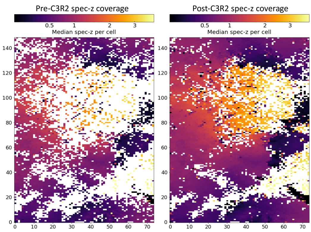
The EDFs (Sect. 4.2.1) and EAFs have their own challenges, with limiting-magnitude requirements of around 26 AB mag over 56 square degrees. The Cosmic Dawn Survey (Euclid Collaboration: McPartland et al., in prep.) is a complementary, UV–IR multiwavelength survey for the EDFs and EAFs that aims to optimise the legacy science returns from these fields, with a primary focus on the high-redshift Universe. The DAWN survey combines dedicated and archival observations from CFHT MegaCam, Subaru HSC, LSST, Spitzer IRAC and other ancillary data available in the EDFs and EAFs, to depths matching the Euclid observations. Photometric catalogues of the imaging data were consistently produced using The Farmer (Weaver et al. 2022). The Spitzer observations and data reduction are described in Euclid Collaboration: Moneti et al. (2022). A description of the ground-based observations from the Hawaii 20 deg2 (H20) Survey and the first catalogue data release can be found in Euclid Collaboration: Zalesky et al. (in prep.).
4.5 Complementary ground-based spectroscopy
As discussed in Sect. 2.2, the correct interpretation of the photometric clustering and lensing signals depends critically on accurate estimates of their redshift distributions. This, in turn, relies on large samples of robust spectroscopic redshifts. To calibrate the redshift distributions of the lenses and sources for the weak lensing and photometric clustering measurements, we have collected a substantial amount of complementary deep spectroscopy.
Our baseline approach is outlined by Masters et al. (2015) and aims to directly calibrate the relation between galaxy colours and the redshift. Specifically, Masters et al. (2015) quantified the expected distribution of galaxy colours using the self-organising map (SOM) algorithm (Kohonen & Honkela 2007), showing that sizeable regions of the colour space were lacking high-confidence spectroscopic redshifts (see the left panel in Fig. 19). They also demonstrated that a targeted campaign of spectroscopic follow-up could obtain the redshifts needed for calibration.
This analysis motivated the Complete Calibration of the Colour-Redshift Relation (C3R2) programme, a coordinated effort between Keck (Masters et al. 2017, 2019; Stanford et al. 2021), the Very Large Telescope (Euclid Collaboration: Guglielmo et al. 2020), and the Large Binocular Telescope (Euclid Collaboration: Saglia et al. 2022), to measure redshifts for faint galaxies down to AB mag spanning the full galaxy colour space. The Keck programme, using DEIMOS, MOSFIRE, and LRIS, resulted in 5100 deep spectra with secure redshifts, while the other observations added over 600 more. The improvement in colour-space coverage as a result of the C3R2 efforts is shown in Fig. 19.
We emphasise that the C3R2 surveys built upon extensive existing spectroscopy to calibrate the colour-redshift relation. Other large-scale deep spectroscopic surveys that contributed substantially to the external redshift calibration sample for Euclid include DEIMOS 10k (Hasinger et al. 2018), DEEP2&3 (Cooper et al. 2012), MOSDEF (Kriek et al. 2015), UDSz (Bradshaw et al. 2013), VANDELS (McLure et al. 2018), VIPERS (Garilli et al. 2014; Scodeggio et al. 2018), VUDS (Tasca et al. 2017), VVDS (Le Fèvre et al. 2013), and zCOSMOS (Lilly et al. 2007).
All deep spectra were collected in a database for careful source-by-source redshift validation, given the need for high purity in the spectroscopic calibration sample (Euclid Collaboration: Ilbert et al. 2021). We are currently testing the performance for the planned tomographic redshift binning for Euclid, using the spectroscopic calibration sample together with the Flagship mock galaxy simulation (Sect. 6.1).
5 Early results from commissioning and PV
Comprehensive results from the commissioning and PV phases will be published once the ongoing data analyses have concluded. The estimated amount of raw data produced by Euclid during the PV phase between August and November 2023 is 21 TB, compared to 12.1 TB of raw data created by HST up until November 2023.171717File names in the HST archive that end in _raw.fits (Matthew Burger, Space Telescope Science Institute, priv. comm.) Therefore, in this paper we present some preliminary results, showing that Euclid’s performance is sufficient for its core scientific goals. More details can be found in the instrument-specific papers for VIS (Euclid Collaboration: Cropper et al. 2024) and NISP (Euclid Collaboration: Jahnke et al. 2024).
5.1 Photometric throughput and molecular contamination
For initial estimates of the total system throughput we used the Gaia (Gaia Collaboration: Vallenari et al. 2023), 2MASS (Cutri et al. 2003), and VHS (VISTA Hemispheric Survey; McMahon et al. 2021) magnitudes of field sources. Considerable colour terms exist in the transformations from the four wide Euclid bands to these external bands (Fig. 12). Our transformations are based on the known passbands and stellar SEDs from our simulations (Sect. 6); in the case of NISP they are given in Euclid Collaboration: Schirmer et al. (2022).
We find the measured NISP and VIS zero points (ZPs) for sources with a frequency-flat SED to be considerably better, by about 0.4 mag, than required. Accurate ZPs and updated Euclid photometric systems will be based on observations of stable white-dwarf spectrophotometric standards that we already established with HST, jointly for Euclid and Roman (proposal ID 16702).
Thin layers of water ice formed on optical surfaces due to outgassing, resulting in throughput modulations from interference and scattering. Contamination is expected and typical for spacecraft, and can be countered with thermal decontamination (for details see Euclid Collaboration: Schirmer et al. 2023).
Throughput monitoring has shown characteristic variations that have been linked to several nanometres of ice on the optics; selective heating of one of the folding mirrors in March 2024 completely restored the transmission to immediate post-launch levels. Because the instrument cavity has little venting area to the outer space, and because outgassing is a continuous process, further decontamination activities are expected over the operation period.
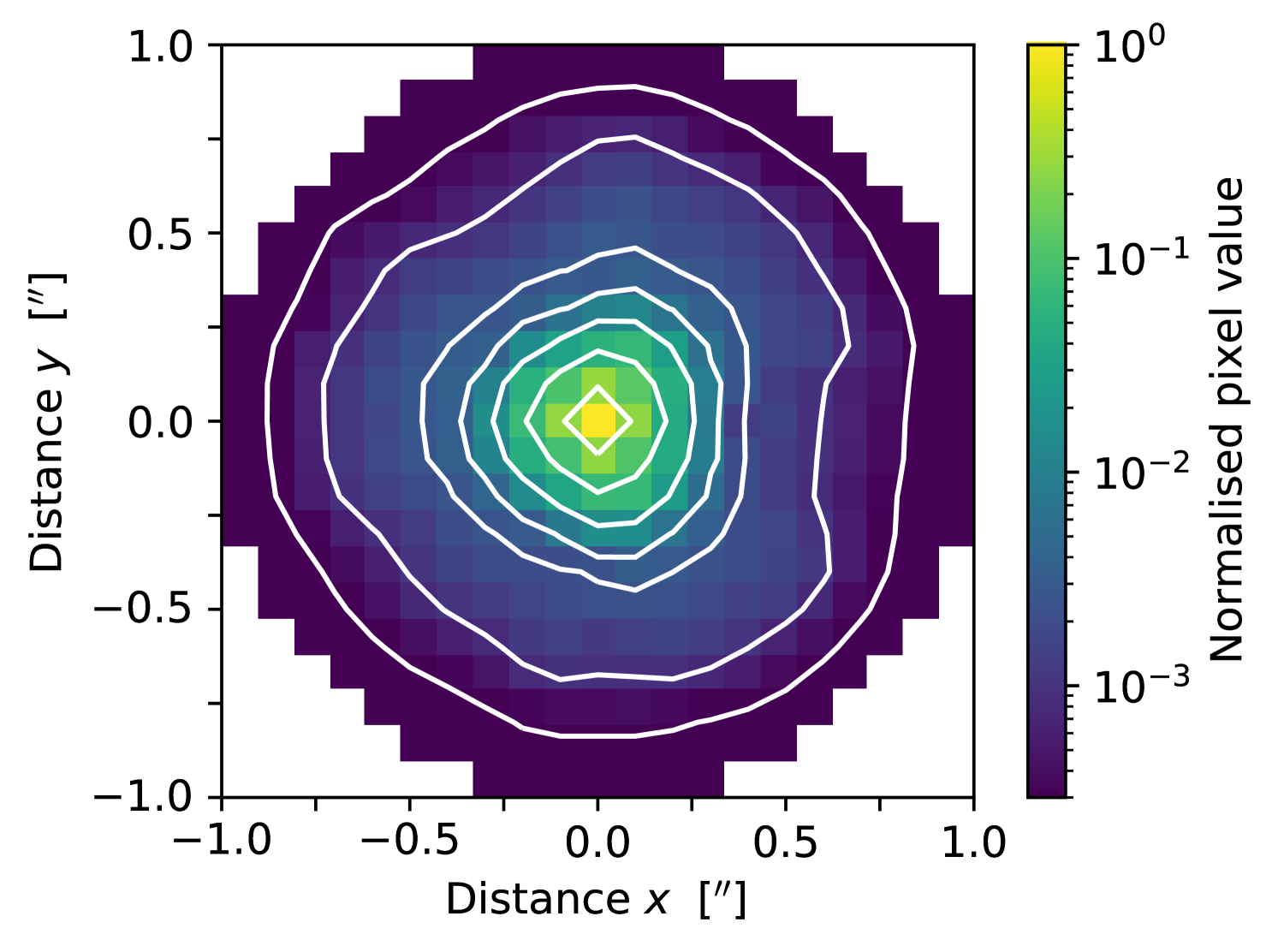
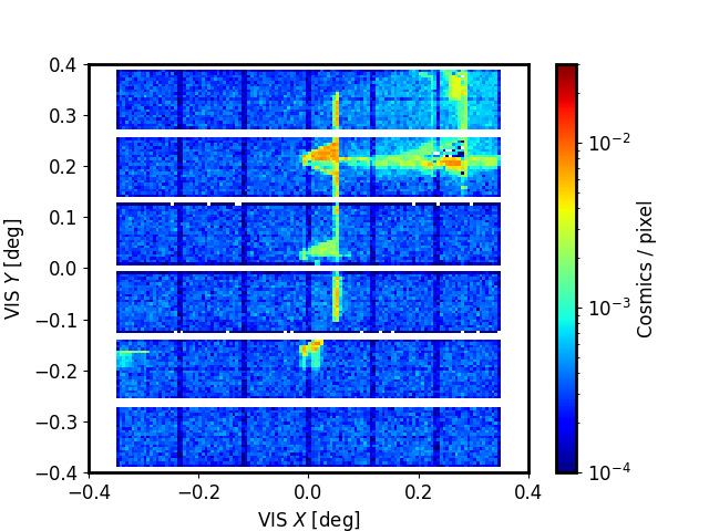
5.2 VIS point-spread function
For the weak lensing measurements we need a detailed and chromatic PSF model that we introduce in Sect. 7.6.4. Here we present an initial and coarse evaluation of the PSF. With a plate scale of pixel-1 the VIS optical PSF is considerably undersampled (Fig. 20). To avoid aliasing in resampled images, the sampling frequency would need to be at least – pixels per FWHM (Bernstein 2002). The requirements on the VIS PSF are an ellipticity less than 0.13, and an FWHM smaller than at 800 nm. The typical ellipticity and FWHM we measure in VIS science exposures are 0.04 and , respectively. This includes jittering effects from the FGS for representative guide-star densities and a background of cosmic-ray hits. The jittering is accounted for in the PSF model using the time-series of the guiding corrections during every exposure. From an opto-mechanical perspective alone, Euclid’s PSF has great stability owing to its SiC components and a thermally stable environment at L2.
In pre-launch testing, the polished M1 was found to have a small residual amount of astigmatism, which would result in a strong dependence of the PSF ellipticity on the telescope’s focus. To reduce this astigmatism, a mechanical correction was applied to M1 to compensate the astigmatism prior to launch. It is thought that this resulted in a small, but noticeable, amount of trefoil in the PSF, visible as an approximately triangular shape in the PSF contours at – from the PSF core (Fig. 20). Like PSF ellipticity, the trefoil is an inherent part of the PSF model (Sect. 7.6.4) and thus accounted for in the shape measurements. The trefoil is described –to leading order– as a spin-3 contribution to the PSF. We therefore do not expect that it has a significant impact on the multiplicative and additive shear biases in Eq. (17), as those are described by spin-0 and spin-4 components.
Thanks to the excellent optical design (see Sect. 3.1.2), most of the light is concentrated in the core of the PSF over the full FoV, while stray light is suppressed. Thanks to further efforts to minimise scattered light (but see Sect. 5.4), the extended PSF should ideally decline with distance as , the limit posed by diffraction. An initial study of the extended PSF by Cuillandre et al. (2024a) took advantage of the observation of the bright star HD 1973. Their results demonstrated Euclid’s exceptional ability for the study diffuse emission around galaxies (see Sect. 10.2), because the extended PSF indeed nearly matches a pure diffraction halo.
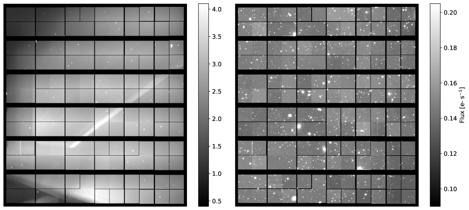
5.3 X-ray contamination from solar flares
Euclid’s instruments have radiation shields, and are additionally protected by the spacecraft itself. This also includes protection from X-rays produced during solar flares, which are absorbed by the silicon in Euclid’s sunshield. However, gaps in the sunshield’s solar cells do let X-rays pass, some of which intersect with the VIS FPA at an angle-of-incidence of about . These are then detected as excess cosmic rays in the VIS images (Fig. 21). NISP is not affected by this.
Contrary to protons that cause displacement damage in the detector’s atomic lattice, X-rays harmlessly create electron-hole pairs in the CCD’s depletion region, like optical photons. The increased density of cosmic rays renders a fraction of the image unusable for scientific analysis. Using the X-ray sensors (XRS; Hanser & Sellers 1996) on board the Geostationary Operational Environmental Satellites (GOES-16 and GOES-18), we find that considerable data loss occurs once the solar X-ray flux approaches about W m-2 in the GOES long band (1.5–12.4 keV).
Typical flares last about 10–60 minutes, so that one or several subsequent VIS images can be affected. As long as particularly active sunspot regions are visible on the Sun, up to 10% of the VIS images can be substantially affected by flares, judging from the GOES solar activity recorded between March and November 2023. During these periods, we expect to lose data from up to 4% of all VIS pixels while passing through the solar maximum in 2024–2025. Any area lost could possibly be recovered during periods of currently unallocated time (Sect. 4.1.2).
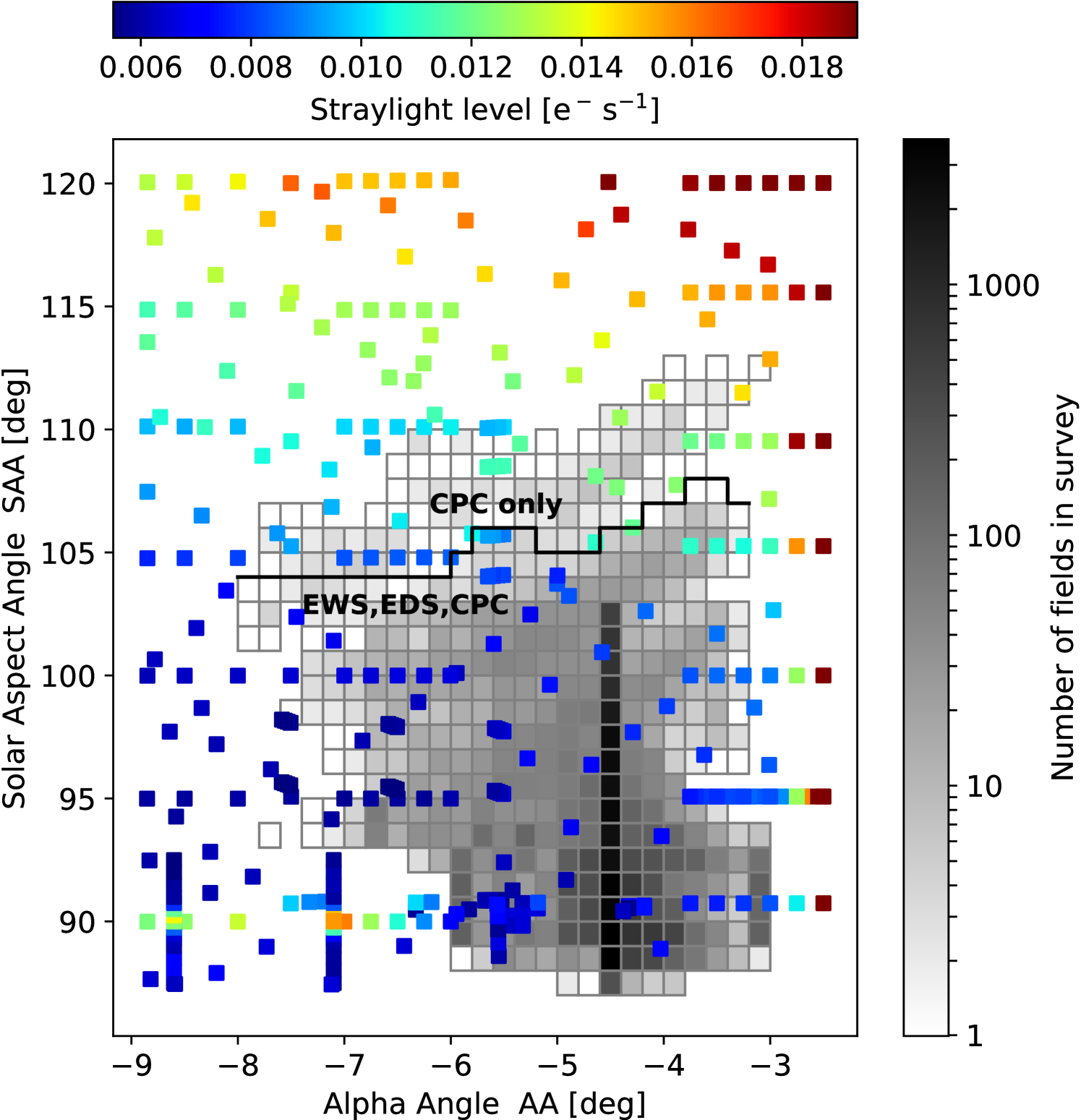
5.4 Optical stray light in VIS
During commissioning it was found that VIS can be affected by considerable amounts of stray light that exceed the zodiacal background by a factor of 10 or more (Fig. 22). The root cause has not been unambiguously identified, but is thought to be a thruster nozzle that is illuminated by the Sun. The light enters the instrument cavity following a triple scattering process, from the nozzle to the backside of the Sun shield, through a hypothesised opening in the thermal multi-layer insulation, to a mounting leg of the VIS shutter, and from there to the VIS focal plane. Even closed-shutter VIS observations are affected, and several parasitic light paths exist. NISP is not affected, as it is enclosed in black multi-layer thermal insulation (MLI), and parasitic light entering through the dichroic is blocked by baffles.
Rotating the spacecraft around its -axis (Fig. 5) imposing moves the nozzle into the shadow, effectively reducing the stray light to levels of a few percent of the zodiacal background (Fig. 22). Rotating up to is safe following a post-launch evaluation. The reduced AA range now available for the survey is (previously ) with a margin of for orbit uncertainty. The stray light is then negligible for Euclid’s core science. Figure 23 shows how the latest survey configuration adapts the spacecraft orientation to the stray light constraint. Low-surface brightness science and some calibrations still require the construction of stray light models from the large number of survey fields and calibration data.
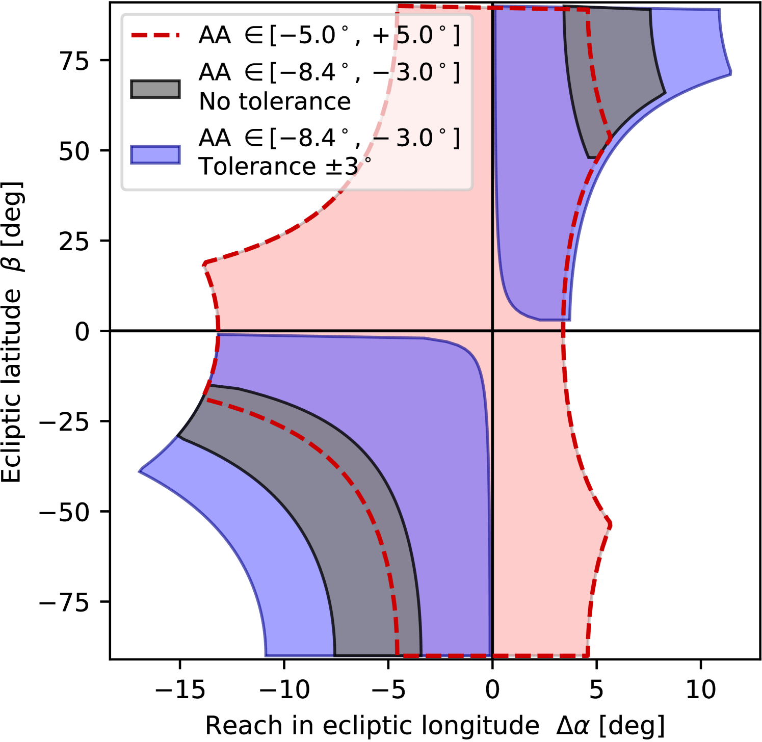
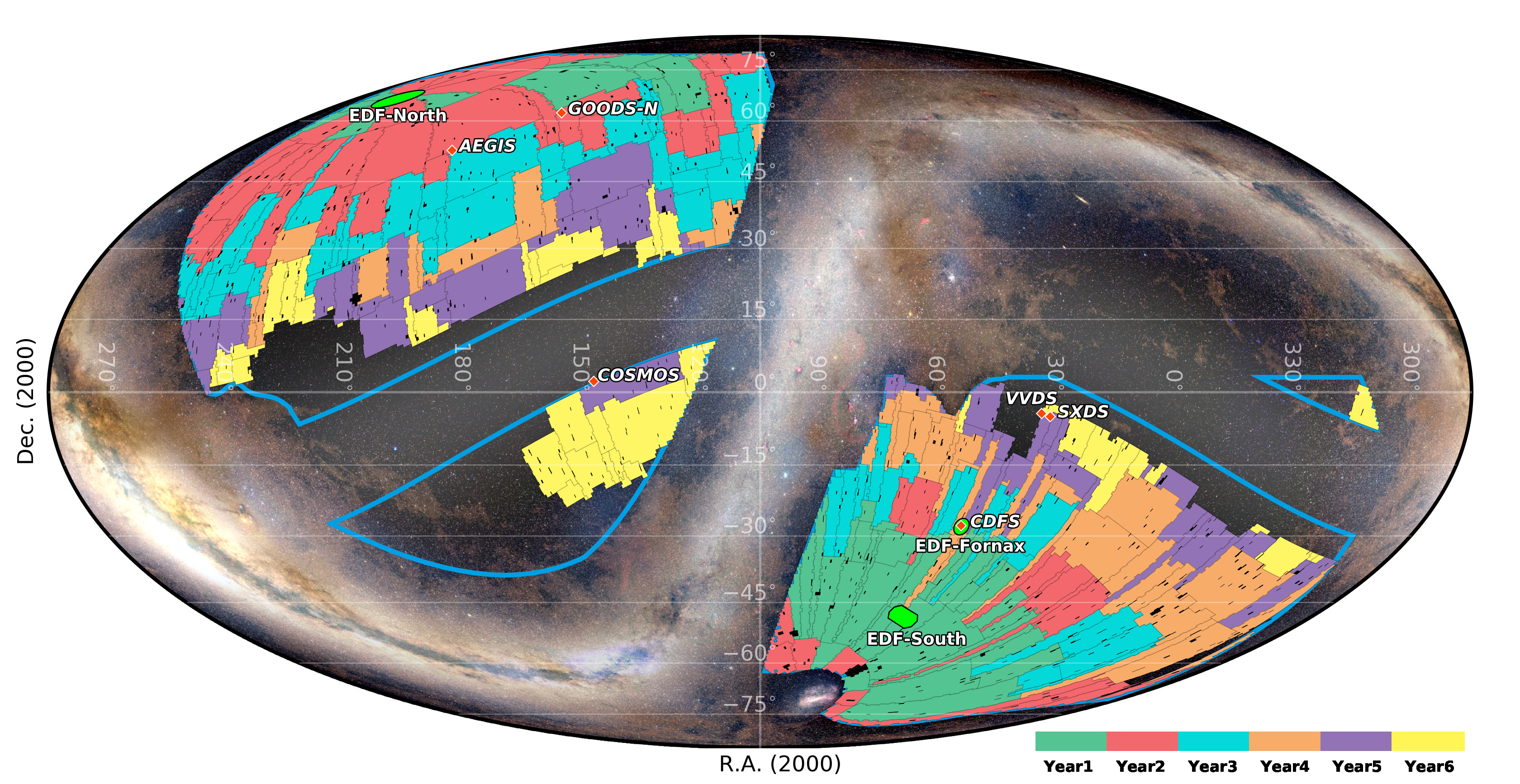
5.5 Latest survey strategy
The reduction of the AA range has the double effect of thinning and skewing the window of visibility, which no longer contains the transit meridian and has a zero reach at some latitudes (Fig. 24). This inhibits the scheduling of Wide Survey patches of any substantial size. Furthermore, half the time it would be impossible to schedule fields with .
Hence, we allowed the FOV to rotate by up to with respect to the tessellation tiles, recovering a large fraction of the tiles’ original visibility, albeit with a different shape. Visibility was regained at all latitudes. A post-launch check showed that we could also safely increase the maximum SAA from to . The new enlarged window of visibility, shown for the leading side in Fig. 24, has two distinct parts in the northern and southern ecliptic hemispheres due to the now asymmetric AA range. The visibilities for the leading and trailing sides are east-west and north-south mirrored. In the leading side, the larger reach in longitude favours observations in the southern hemisphere, while the trailing side favours the northern hemisphere.
This relaxed tessellation constraint implies that neighbouring FoVs are no longer necessarily aligned. To avoid gaps between FoVs we tessellate the sky with smaller tiles, increasing the mean overlap between fields, which reduces the covered sky area. In the latest survey computation, Fig. 25, the EWS covers 13 416 deg2 of which 171 deg2 are lost due to bright stars. The effective sky area is 13 245 deg2, representing a decrease of 5% as compared to the target of 14 000 deg2 in 6 years (Sect. 4.1). The implications of this reduction in survey area for the core science objectives, as well as possible mitigation strategies are being explored.
6 Simulated data
The calibration observations discussed in Sect. 4.3 provide important information about the performance of the telescope and the data that are collected. To prepare the pipeline and to interpret the results, simulated data are needed as well. This includes large realistic input universes that can capture survey characteristics, such as the Euclid Flagship Simulation (EFS; Sect. 6.1) as well as sophisticated pixel-level instrument simulators (Sect. 6.2). The latter are essential for exploring the sensitivity of the measurements to instrumental effects and test our ability to correct these.
6.1 The Euclid Flagship Simulation
The optimal exploitation of the Euclid data demands the development of large-volume and high-mass resolution numerical simulations that reproduce the large-scale galaxy distribution that the mission will observe with high fidelity. Not only do these help to assess the performance with a realism that cannot be achieved otherwise, but such simulations are also an essential tool for the development of the data processing and science analysis pipelines. The major advance that the Euclid data will bring implies the need for a dedicated effort. To this end, we developed the EFS, which is described in detail in Euclid Collaboration: Castander et al. (2024). Here, we summarise its main characteristics.
The EFS features a simulation box of 3600 Mpc on a side with particles, leading to a mass resolution of . This 4 trillion particle simulation is the largest -body simulation performed to date and matches the basic science requirements of the mission, because it allows us to include the faintest galaxies that Euclid will observe, while sampling a cosmological volume comparable to what the satellite will survey. The simulation was performed using PKDGRAV3 (Potter & Stadel 2016) on the Piz Daint supercomputer at the Swiss National Supercomputer Center (CSCS). The input cosmology differs slightly181818The EFS uses the following values for the density parameters: ; ; and , with a radiation density , and a contribution from massive neutrinos . Additional parameters are: the equation of state of dark-energy ; the reduced Hubble constant ; the scalar spectral index of the initial fluctuations ; and the scalar power spectrum amplitude (corresponding to ) at . from the one listed in Table 1, but this has no material impact on the applications.
The initial conditions were realised at with first-order Lagrangian perturbation theory (1LPT) displacements from a uniform particle grid. The transfer functions for the density field and the velocity field were generated at this initial redshift by CLASS (Lesgourgues 2011) and CONCEPT (Dakin et al. 2022). As the usual scaling of the linear power spectrum at to the initial redshift of the simulation (known as back-scaling), to generate the initial conditions, was not used, all linear contributions from radiation, massive neutrinos, and metric perturbations (in the -body gauge, see Fidler et al. 2015) were included via a lookup table and applied as a small corrective PM (particle-mesh) force at each timestep. This ensures a match to the linear evolution of the matter density field at all redshifts when including these additional linear terms. The main data product was produced on the fly during the simulation and is a continuous full-sky particle light cone out to , where each particle was output exactly when the shrinking light surface sweeps by it. This resulting ball of particles contains 31 trillion particle positions and peculiar velocities (700 TB of data). The 3D particle lightcone data were used to identify roughly 150 billion dark-matter halos using Rockstar (Behroozi et al. 2013), and to create all-sky dark-matter 2D maps in 200 tomographic redshift shells between and , with a HEALPix (Górski et al. 2005) tessellation resolution , corresponding to per pixel.
The halo catalogue and the set of 2D dark-matter maps are the main inputs for the Flagship mock galaxy catalogue. A detailed description of the catalogue production is given in Euclid Collaboration: Castander et al. (2024), which we summarise here. Galaxies were generated following a combination of halo-occupation distribution (HOD) and abundance matching (AM) techniques. Following the HOD prescription, halos were populated with central and satellite galaxies. Each halo contains a central galaxy and a number of satellites that depends on the halo mass. The halo occupation was chosen to reproduce observational constraints of galaxy clustering in the local Universe (Zehavi et al. 2011).
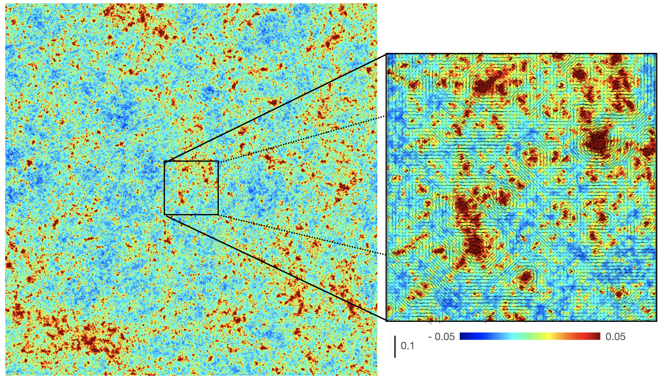
The luminosities of the central galaxies were assigned by performing abundance matching between the halo mass function of the simulation halo catalogue and the galaxy luminosity function (LF). We took as the reference luminosity function a parameterised prescription that tries to fit the observed LF throughout the redshift range of the simulation. We then applied a 15% scatter to the resulting luminosities. The application of scatter is necessary to reproduce the galaxy clustering dependence on luminosity. The satellite luminosities were assigned assuming a universal Schechter LF for satellites in which the characteristic luminosity depends on the central luminosity in a way that ensures that the global luminosity function agrees with observations. Galaxies were split into three colour types, namely red, green and blue, and the central and satellite galaxies in each group were distributed to match the observed clustering as a function of colour by Zehavi et al. (2011). The radial positions of the satellites within their halos follow Navarro–Frenk–White (NFW) profiles (Navarro et al. 1997) with each colour type having its own concentration: green and blue galaxies are distributed using a concentration that is respectively one-half and one-quarter times that of the red galaxies, consistent what Collister & Lahav (2005) found for blue versus red galaxies in the nearby Universe. This colour segregation is assumed to hold at all redshifts (see Sect. 10.6 for a discussion of this assumption).
To determine the simulated redshifts, we assumed that the central galaxy is at rest in its halo. The satellite velocities were drawn using formula derived by solving the Jeans equation of local dynamical equilibrium for each type, assuming velocity anisotropy profiles consistent with what was measured from the kinematics of low-redshift regular clusters (Mamon et al. 2019), with green and especially blue galaxies having more radial orbits around their host haloes. Redshifts of the galaxies were then obtained by projection of these 3D velocities along the LoS.
SEDs were assigned to each galaxy with a procedure that aims to mimic the observed colour distributions as a function of redshift. The resulting SEDs are a linear combination of the ones presented in Ilbert et al. (2009). The stellar masses were computed from the galaxy luminosities and the mass-to-light ratios of the SEDs. The star-formation rates were computed from the ultraviolet luminosity of the SED. The luminosity of the H line was computed from the star-formation rate following the Kennicutt recipe (Kennicutt 1998a). The galaxy clustering measurements of Euclid rely on the detection of this line in the galaxy spectra (see Sect. 2.1). We therefore want to simulate their distribution to our best current knowledge. Consequently, we then refined the H luminosities to match the models of Pozzetti et al. (2016), using abundance-matching techniques. The luminosities of the other main emission lines were assigned using observed relations, taking the H line as reference. The shapes and sizes of the galaxies were assigned following relations based on HST observations (Miller et al. 2013; Dimauro et al. 2018). The observed fluxes of each galaxy were computed by integrating the SED with the filter transmission for the surveys that are expected to be used to obtain photometric redshifts.
As for galaxy lensing properties, we followed the ‘onion universe’ approach presented in Fosalba et al. (2008) and Fosalba et al. (2015), to compute all-sky weak lensing observables (convergence, shear, and deflection) within the Born approximation. The latter agrees within 0.1% out to a multipole with the much more complex and central processing unit (CPU) time-consuming ray-tracing technique (Hilbert et al. 2020). Figure 26 shows the convergence (colour-coded) and the overlaid shear field (sticks indicating the amplitude and direction of the shear) for a source redshift in a patch of approximately of the EFS.
6.2 Simulated Euclid data
Pixel image simulations serve as test data for the development of the data-processing pipeline and computing infrastructure, and to validate the stringent requirements regarding performance and data quality (e.g. Euclid Collaboration: Gabarra et al. 2023). In this respect, several end-to-end science performance verification (SPV) tests have been performed throughout the mission preparation, which allowed for the reproduction of certain instrumental issues to assess their impact and guide decision making (see Sect. 8.1 for more details). Image simulations have also been essential to develop alternative solutions to critical problems that were discovered during on-ground tests, such as the non-conformity of one of the three red grisms for the NISP instrument (Euclid Collaboration: Scaramella et al. 2022; Euclid Collaboration: Jahnke et al. 2024); or to evaluate the impact of unexpected features discovered in-flight, such as the contamination of VIS images by X-ray photons during solar flares (see Sect. 5.3 and Fig. 21). Finally, image simulations are necessary to calibrate intrinsic biases related to the methods used to measure the shapes of the galaxies in the cosmic shear analysis. A large volume of very accurate and representative simulations is required to determine these biases to the required level of precision (e.g. Hoekstra et al. 2017).
To ensure a common input for the instruments, the starting point is a ‘true universe’ catalogue that contains all input sources and their corresponding parameters, spectra, and shapes. These parameters are based on the output from the EFS (Sect. 6.1), which provides both spectra (continuum and emission lines) and morphological parameters (bulge and disc models). The stars are simulated using a hybrid catalogue, using actual stars from Gaia DR3 (Gaia Collaboration: Vallenari et al. 2023) at the bright end (), merged with the fainter end of deep stellar population simulations using the Besançon model (Robin et al. 2003; Czekaj et al. 2014; Lagarde et al. 2021), including binaries, down to . All objects are simulated using common coherent libraries to ensure consistent results between the simulated VIS imaging, NISP photometry and spectroscopy, and ground-based imaging. In addition to individual sources, the simulations include zodiacal light, diffuse stray light from stars beyond the simulated pointing, and thermal irradiance caused by the heat of the various elements of the telescope and instruments. The instrument models and the reference survey characteristics are drawn from the central mission database. This database (versioned and controlled by dedicated change control boards) provides the instrument simulators with all the parameters necessary to simulate the numerous instrumental features of each simulation channel.
To create simulated VIS observations and the associated calibration frames, we have developed the Euclid VIS simulator (ELViS). It includes an accurate emulation of the optical response, which is based on the complex PSF modelling tools that are described in Sect. 7.6.4. Although challenging, ELViS can capture the complexity of the chromatic PSF and its spatial variations. The sources are projected on the simulated mosaic of 36 CCDs, and an extensive list of instrumental signatures can be included, such as bias, pixel response non-uniformity, cosmetic defects, saturation, bleeding, shutter movement, and ghosts from the dichroic plate. Particularly important for Euclid are simulations of the imperfect charge transfer during the readout. The simulated readout electronics include a nonlinear response, saturation of the analogue-to-digital converter, and electric cross-talk, with parameters determined during the on-ground test campaigns.
To capture the dual use of the NISP instrument, two separate codes are used, Imagem and TIPS, to simulate the photometric and spectroscopic channels, respectively. As is done for VIS, both science and calibration images are produced. As the photometric and spectroscopic channel share the same optical path and detector units, the NISP-P simulator, Imagen and NISP-S simulator, TIPS employ common background, PSF, optics, detector, and electronics models. Consistency across the two channels is particularly important because the spectroscopic analysis relies on measurements from the imaging data. The simulations start from the same list of astronomical sources that is used by ELViS. The simulated NISP PSFs contain the same types of effects that have been included for VIS instrument, but with a simplified module to capture the variation of the PSF (given the less strict requirements, we opted to use a tabulated PSF as opposed to recomputing it for each object). Each different multiple accumulated sampling readout (MACC mode) is simulated for photometric and spectrometric images. At the detector level, variable QE is simulated using QE estimates obtained from on-ground tests, while the pixel-response non-uniformity (PRNU) is taken from the on-ground flatfield data. To capture biases introduced during readout, nonlinearity and gain are simulated together with the MACC readout modes. On the spectroscopic side (TIPS simulator), the slitless light dispersion is handled by aXeSIM191919http://axe-info.stsci.edu/axesim/ (Kümmel et al. 2009), developed by the Space Telescope Science Institute. The simulation of the slitless spectra requires a complete characterisation of the trace dispersion, with sensitivity, diffraction coefficients, grism tilts, vignetting, and PSFs at each dispersion order (expressed as a Taylor series expansion). The dispersion order of interest is the first order, where the main spectrum can be recovered. However, the zeroth and second orders of dispersion need to be simulated as well. The readout electronics are shared with the photometric channel and the simulations are therefore also similar (except for the MACC modes, which are photometry and spectroscopy specific).
We also produce pixel simulations of the external ground-based surveys that are used to characterise the SEDs of the stars and galaxies and to determine photometric redshifts. Here, it is important to capture the key characteristics of the ground-based data, summarised in Sect. 4.4, while providing realistic images that can be used to examine the performance of the various processing steps. With the exception of LSST, the surveys have already collected data, so that realistic prescriptions for their main features can be readily implemented. For instance, the simulations include realistic values for the background levels, zero points, filter transmissions, bias levels, flat-field characteristics, detector defects, observed cosmic rays, and PSFs for each of the simulated surveys. Importantly, the simulated ground-based data use the same input catalogues as the simulations of the Euclid instruments, so that all the detection and cataloguing steps can be tested, as well as the determination of photometric redshifts. For a more detailed description of the pixel simulations, the reader is referred to Euclid Collaboration: Serrano et al. (2024).
7 Survey data products
Euclid provides high-quality optical and NIR imaging, as well as slitless NIR spectroscopy over a large fraction of the extragalactic sky. The processing of these data and supporting ground-based observations is performed by the SGS. In this section, we present the most salient parts of the pipeline. The key steps in the processing of the Euclid optical and NIR imaging data are highlighted in Sects. 7.1 and 7.2, respectively, while the processing of the supporting ground-based imaging is summarised in Sect. 7.3. These data form the basis for the creation of the object catalogues, described in Sect. 7.4. The processing of the slitless spectroscopy and the subsequent redshift determination are discussed in Sect. 7.5.
In Sect. 7.6 we describe how these results are used to derive the key ingredients for the 3×2pt analysis. The science-ready data products, summarised in Sect. 7.7, include the various two-point statistics, as well as weak lensing convergence maps and catalogues of clusters of galaxies. Although many of these data products are excellent starting points for myriad scientific investigations, several high-level data products will be released as well, with a particular focus on the interpretation of the primary probes. These data, as well as a range of calibrated data products, will be released to the scientific community in a number of data releases (Sect. 7.8).
7.1 Processing of VIS imaging data
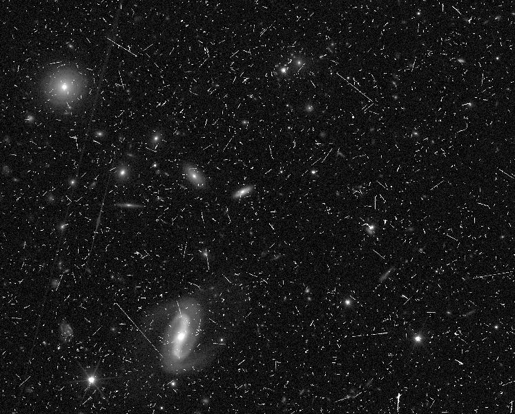
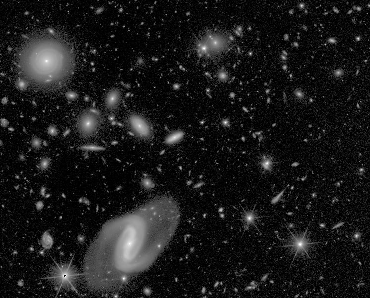
The high resolution imaging data provided by the VIS instrument is the starting point for the weak lensing measurements. To reach the main objectives of Euclid, the shapes of about 1.5 billion galaxies need to be measured with unprecedented accuracy. To this end, a range of instrumental effects need to be carefully accounted for (Massey et al. 2013; Cropper et al. 2013; Euclid Collaboration: Paykari et al. 2020). This involves fully characterising the performance of the instrument through the processing and analysis of an extensive amount of calibration data. The subsequent processing of the raw VIS data relies on these calibration products to correct all relevant instrumental effects to enable robust shape measurements.
Before launch, each pipeline processing element was tested and validated using the simulations described in Sect. 6.2. These simulations enabled an assessment of how well instrument models (based on pre-launch observations) could be derived using realistic observing sequences. They also allowed an evaluation of how well measurements (photometry, astrometry, and object shape) could be made after the application of these models. These findings are being updated using the PV observations and in-flight calibrations.
At its most basic level, the processing of the VIS data can be divided into three categories: the calibration pipeline that generates or updates the VIS calibration models, which by definition do not alter the input pixels; the science pipeline that alters the input pixels by applying the calibration models; and the validation pipeline designed to assess the performance of the data processing. Because the requirements for weak lensing shape measurement are so strict, the adopted approach is to apply the minimal number of pixel-level corrections, and, if feasible, to provide the information to reverse the correction if necessary (or to provide images for which a given correction has not been applied).
In detail, the pipeline that processes the VIS data calibrates and corrects a comprehensive set of pixel-level effects, which would otherwise bias the shear estimation (Cropper et al. 2013). These include electronic offset (bias), dark current, PRNU, detector-chain nonlinearity, brighter-fatter effect (Antilogus et al. 2014), charge-transfer inefficiency (Israel et al. 2015), illumination correction, and the flagging of cold, hot, and saturated pixels, as well as optical and electronic ghosts and cosmic rays. Moreover, the astrometric solution, required to be better than 30 mas, and photometric solution are computed, using Gaia DR3 (Gaia Collaboration: Vallenari et al. 2023) as the reference catalogue. Apart from robust shape measurements, these processing steps enable relative photometry measurement with an accuracy better than 1%. This implies that the collective contribution of residuals from the detection chain, small- and large-scale flat fielding, source extraction, and background and scattered light correction, is smaller than this target.
The main outputs of this step in the processing are the calibrated individual exposures, as well as stacks and their associated source catalogues. However, important supporting data are also provided, such as the calibration models, the background and flag maps, the distortion model, and a first estimate of the PSF model that is used for multi-band photometry during the generation of the main survey catalogue (Sect. 7.4). For reference, Fig. 27 displays a view of a single raw frame (left) and the corresponding processed stack (right) of the Euclid self-calibration field. The left panel demonstrates the need for the robust detection of cosmic rays, whereas the deep image on the right shows the potential of Euclid to study low-surface-brightness features around galaxies.
7.2 Processing of NIR imaging data
The interpretation of the observed weak lensing signal requires accurate estimates of photometric redshifts (Sect. 2). As shown by Abdalla et al. (2008), the NIR images from the NISP instrument in the , , and bands provide key information to improve the photometric redshift precision (see also Sect. 7.6.1). To reach this goal, NISP images require an exquisite calibration that takes into account all instrumental effects and a possible time variation of the telescope’s throughput (Sect. 5.1). Most notably, the relative photometric calibration needs to be better than for the entire magnitude range down to 24.0 AB. This requirement has been the main driver for the design of the processing pipeline.
The generation of the calibration products needed for the reduction of NISP images is carried out through a number of dedicated pipelines running on well-defined blocks of calibration observations. This is the case, for instance, for bad pixel identification, dark current, detector nonlinearity, PRNU, large-scale illumination correction, geometric distortions, persistence image creation, and relative and absolute photometric calibration factors.
The reduction of the NIR exposures can be divided into three main steps: the preprocessing, where all detector-related effects common to both NISP photometric and spectroscopic exposures are accounted for; the calibration part, which includes PSF estimation, computation of the astrometric solution based on VIS catalogues, application of flat-fielding and photometric calibration based on the precomputed products, and source catalogue extraction from individual dithered observations; and lastly the stacking of frames for each observation sequence along with the generation of their PSF and source catalogues. Similarly to the VIS processing, we keep the amount of pixel-level operations to a minimum, while providing at the same time all relevant information about modelling and corrections, so that they may be reversed if needed or tailored for specific purposes.
For each of the three NIR filters, the output of the NIR processing consist of calibrated individual dithered observations and stacks with their associated source catalogues. These data products are provided to the subsequent processing step for the creation of the main survey catalogue (Sect. 7.4), along with all ancillary information, including root mean square (RMS), data quality flags, background, and PSF images.
Prior to launch, the design and implementation of the various processing steps have been extensively tested through a number of simulation campaigns with increasing realism and coverage of instrumental features, mostly based on modelling from ground calibration campaigns and in some cases by design. Further improvements will be made using the calibrations obtained during the PV phase (Sect. 4.3.1). Figure 28 gives an impression of the quality of data. It shows a small area in the Euclid self-calibration field (Sect. 4.2.3).
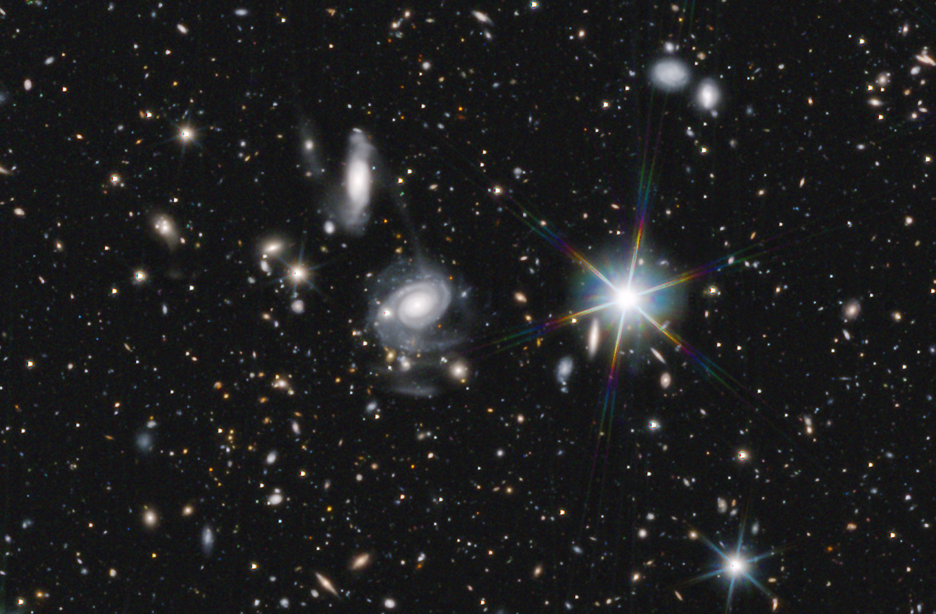
7.3 Processing of ground-based imaging data
The Euclid imaging data are complemented by supporting ground-based observations (Sect. 4.4) to improve the precision of the photometric redshifts and to determine the SED-weighted PSF model for the galaxies used in the weak lensing analysis (Sect. 7.6.3). The challenge is to uniformly calibrate this vast and heterogeneous external data set with extraordinary accuracy: the EWS is composed of three surveys (UNIONS, DES and the LSST) employing five telescopes with differing , , , , and filters. The EDS and EAFs have primarily been observed using HSC, but there are additional datasets available featuring, for example intermediate band filters, that are being included to aid in the testing and validation of the photometric redshift estimation and the VIS PSF modelling. Hence, the data are complex, with a wide range of single exposure depths and seeing conditions (from roughly to ), sampled with over 450 different detectors. The resulting data set will be large, ultimately comprising roughly 1.5 PB of raw (uncompressed) science observations. Crucially, to ensure robust photometric redshifts, the processing of these data should result in 1% single-filter photometric homogeneity over the entire EWS, and subpercent colour homogeneity over the VIS FoV (Eriksen & Hoekstra 2018).
For the cataloguing process described in Sect. 7.4, the required external data product inputs are coadded ground-based images. These coadded images are supplemented with associated PSF models for all objects that are identified in the VIS- and NIR-based detection process. These coadded images are built using a single pipeline whose software components were initially developed as part of the DES data management system (Mohr et al. 2008) and have been tuned and validated to serve our needs and then integrated into the SGS code base. The pixel coaddition is based on the widely used SWarp code (Bertin et al. 2002; Bertin 2010). We developed a dedicated code to model the PSF to take into account the position-dependent PSF models of all input images.
To facilitate the processing of the individual ground-based exposures, a common data model is enforced across all external ground-based data sets. This common input data product– termed a single-epoch frame (SEF)– consists of a detrended and astrometrically and photometrically calibrated single CCD image, the associated position-dependent PSF model and an associated catalogue that includes, at a minimum, the sky positions and PSF-fitted magnitudes of the brighter, unresolved sources. Typically, these SEFs are created using output data products from the external surveys. For example, the ensemble of -band SEFs from Pan-STARRS is prepared using the software within the Pan-STARRS collaboration (Magnier et al. 2016; Waters et al. 2016). Similarly the - and -band SEFs from WHIGS and WISHES are produced using output data products from HSCpipe (Bosch et al. 2018, 2019), which is software developed by the HSC and LSST teams. The - and -band SEFs from CFHT are created using the MegaPipe software developed by the CFHT team (Gwyn 2008).
For the EDS data, we receive the ground-based data from the Cosmic Dawn team (Euclid Collaboration: McPartland et al., in prep.; Sect. 4.4) in the case of Euclid Deep Field North (EDF-N) and Euclid Deep Field Fornax (EDF-F), while we directly downloaded public data from the HSC archive for other EAFs such as COSMOS and produce the data ourselves in the case of Euclid Deep Field South (EDF-S). For the publicly available DES data (Abbott et al. 2018b) and other Dark Energy Camera (DECam) (Flaugher et al. 2015) data, we produce and calibrate the SEFs ourselves using extended versions of pipelines originally developed for DES (Mohr et al. 2012; Desai et al. 2012) that include also image masking (Desai et al. 2016) and have been reorganised and rewritten to simplify the large-scale processing required. Finally, thanks to a collaboration agreement, the data products from the LSST are provided through a joint Euclid-Rubin working group (see Guy et al. 2022, for details).
To enable an accurate and uniform photometric calibration of the ground-based external data across the full extragalactic sky that will be observed by Euclid, we leverage Gaia (Gaia Collaboration: Prusti et al. 2016) photometry and spectroscopy that are stable across the sky with a systematic uncertainty of 2 mmag (Gaia Collaboration: Vallenari et al. 2023). Initial testing of statistical transformations from Gaia , and to each of the external bands in DES demonstrated a high level of consistency between the DES DR2 (Abbott et al. 2021) calibration and the Gaia-based predictions (George et al. 2020). Further tests with the UNIONS dataset provided indications that the external photometry predictions from statistical transformations based on Gaia , and photometry exhibited improved stability across the sky and improved internal self-consistency in comparison to the original UNIONS calibration. This demonstrated the promise of adopting Gaia data as a basis for calibrating the heterogeneous ground-based data sets to ensure consistent photometric redshifts and stellar SED s across the Euclid sky.
A challenge in employing the statistical transformation function from Gaia , and (George et al. 2020) to the external data bands is that systematic changes in the stellar populations over the Euclid sky could bias the Gaia-based predictions, introducing errors larger than the advertised 2 mmag systematic uncertainties in Gaia photometry. Therefore, with the availability of the Gaia DR3 (Gaia Collaboration: Vallenari et al. 2023) and calibrated spectra, we have transitioned to using Gaia spectra and the associated synthetic magnitudes to calibrate the external data. We calculated Gaia synthetic magnitudes using the Gaia calibrated spectra together with the appropriate bandpass for each external survey band and camera combination. Under the assumption that the external data bandpasses are robust, these Gaia synthetic magnitudes are highly accurate, enabling us to meet the Euclid requirements. In the case that there are significant residual errors in the external data bandpasses, these errors would enter both the ground-based photometric calibration and the SED fitting being performed for photometric redshifts and stellar SED constraints. In addition, we expect to be able to use the Gaia spectra to aid in characterising bandpass variations across the focal plane in the ensemble of cameras being used to obtain the ground-based data needed for Euclid.
For the UNIONS and DES external data sets there are enough Gaia synthetic magnitude constraints per SEF to enable a photometric calibration of individual SEFs that approaches the 2 mmag systematic floor of the Gaia mission. For the EDS and EAF data sets, the situation is more complicated, because the typical HSC integrations are longer, pushing the saturation limits in these SEFs to fainter magnitudes and reducing the overlap between the Gaia-based synthetic magnitudes and the external data sets. To address this we incorporate also relative photometric constraints between overlapping pairs of SEFs. This allows us to combine the direct photometric constraints from Gaia synthetic magnitudes across an ensemble of co-located SEFs, delivering a comparable level of photometric calibration accuracy in the EDS and EAF datasets as we achieve in the EWS.
7.4 Catalogue creation
The imaging data form the basis of the object catalogue that is used for most of the subsequent analyses. To avoid multiple entries for the same object, the survey area is divided into predefined tiles. Each tile consists of a rectangular extended area and a core area that is defined by a set of HEALPix indices (Górski et al. 2005). All data needed for the detection and photometry are generated to cover the extended tile area, which overlaps with neighbouring tiles. Only the objects in the core area, which is unique for each tile, are actually selected for insertion into the object catalogue (Kümmel et al. 2022). This procedure avoids multiple detections of identical objects in adjacent tiles, while allowing the proper processing of large, extended objects in the overlap areas between two tiles.
The pipeline retrieves all imaging data for the tile of interest and creates coadds of the calibrated Euclid VIS and NISP exposures. As part of this step, the background is subtracted from each exposure and each image is sampled to the native VIS pixel scale of pixel-1. Information on flagged pixels and areas around bright stars that are affected by diffraction spikes or blooming is propagated, as is the case for the model PSF in each exposure.
In principle, the information in all bands could be combined to maximise the prospects for object detection, but this would result in complex selection biases for the primary probes. To avoid this, we opt for a staged process, where we detect and subsequently deblend objects in the VIS and NIR bands separately. This ensures a clean selection of the weak lensing source sample, while recording all objects that are visible in the Euclid data. For the NIR detections we employ a deep image generated from the combined , , and data. Source detection is done with SourceXtractor++202020https://github.com/astrorama/SourceXtractorPlusPlus (Bertin et al. 2020), with detection parameters that are optimised for completeness, while keeping the false detection rate below . The denclue algorithm (Tramacere et al. 2016) is used for the deblending procedure. The resulting VIS and NIR detections are then combined into a single joint catalogue that is used to perform photometry and to determine a number of other properties. To enable the selection of VIS-detected objects, the combined catalogue contains a flag that indicates whether a source was detected in VIS or in the deep NIR image.
Accurate multi-band photometry is essential for the determination of robust photometric redshifts, but optimising the pipeline for this application might not be ideal for other science cases. Therefore, to maximise the usefulness of the catalogue, fluxes are measured in the following ways.
-
•
Total object flux within a Kron aperture on the detection image with T-PHOT212121The transformation of the PSF from the VIS band with the highest resolution to the NIR and ground-based images, which is necessary for A-PHOT and T-PHOT, is done using convolution kernels as described in Boucaud et al. (2016). (Merlin et al. 2015).
-
•
Isophotal flux measured by summing the flux of the pixels above the detection threshold in the detection image.
-
•
PSF flux measured on the VIS image.
- •
-
•
Template-fitting photometry computed by PSF-convolving the VIS object shape to the different bands and fitting the surface-brightness profiles.
-
•
Single-Sérsic fitting photometry using SourceXtractor++ (Kümmel et al. 2022) in all available bands.
To increase the scientific value of the catalogues, morphological properties are also determined. A robust separation of point-like and extended objects is achieved by computing the difference between the central surface brightness and the total brightness. This quantity is translated to a probability of the object being point-like using calibrations based on simulated data (Sect. 6.2). We include the non-parametric estimates for concentration, asymmetry and smoothness (CAS; Tohill et al. 2021), as well as the Gini index (Lotz et al. 2004) for all objects. Moreover, the catalogue includes the best-fit Sérsic models in all bands obtained using SourceXtractor++ (Kümmel et al. 2022).
7.5 Processing of NIR spectroscopy data
The first steps in the processing of the dispersed NIR images are similar to what is done with the imaging data used for photometry (Sect. 7.2): the same detector-level effects need to be accounted for (bad pixel flagging, nonlinearity correction, persistence masking, dark subtraction, and cosmic-ray rejection). Therefore, these steps are based on a common set of processing elements. The different nature of the images does lead to some modifications, for instance in the cosmic ray rejection. The main difference, however, pertains to the instrument models that are adopted for the two observing modes. Specific calibration products are used for each case. The resulting images are then used to extract the spectra.
7.5.1 Extraction of spectra
To extract the spectra from the preprocessed NISP spectroscopic images, we need to precisely locate the dispersed image of each object (the so-called ‘spectrogram’) in the spectroscopic frame. Specifically, we are interested in the first order of the grism dispersion, where more than 96% of the object flux is concentrated. To this end, the object catalogues derived from the corresponding direct photometric images are critical.
First, the two-dimensional first-order spectrograms for each object are located on the full NISP spectroscopic frame, based on its coordinates measured from the corresponding direct image. This involves applying the astrometric solution, which translates sky coordinates into detector reference positions of the different dispersion orders. The precise location of the spectrogram is then traced, accounting for any inclination and curvature. Along the dispersion direction, the spectrum is re-mapped into wavelength steps, using the wavelength solution computed from reference planetary nebulae emission-line spectra (see Sect. 4.3.1, and Euclid Collaboration: Paterson et al. 2023).
Detector-level pixel-to-pixel variations are corrected from calibrated detector flats, and values for the background over the full focal plane are sampled on detector areas where no spectra are present. These are then averaged per detector, and the values subtracted over the whole frame.
In slitless observations, overlapping spectra from nearby objects represent an important contribution to the noise affecting a given spectrum. Euclid adopts a specific observing sequence to mitigate this, collecting four exposures at varying dispersion directions in each ROS, as described in detail in Sect. 3.5.3. A model of the spurious contribution of each neighbouring source contaminant is built using its spatial extent estimated from the -band photometric image, and its intrinsic SED. If possible, the latter is estimated from uncontaminated portions of the spectrograms extracted from one of the available exposures taken as part of the ROS. If an object happens to be contaminated in all four exposures, a power-law SED interpolation of the available NIR photometric measurements is used instead. These decontamination operations are performed on each identified 2D spectrogram, ultimately resampled on a rectilinear grid along the dispersion and cross-dispersion directions.
At this stage, 1D spectra can then be extracted from the individual exposures in a ROS by properly integrating over the cross-dispersion dimension. This is performed through optimal extraction (Robertson 1986; Horne 1986), using a weighting profile derived from the -band photometric image of the source. This also includes appropriate rotation, matching of both NISP-P and NISP-S PSF s, shear, and resampling, to account, in the case of galaxies, for the inclination of the source with respect to the dispersion direction, so as to minimise effective spectral line-spread function and maximise S/N.
The spectrum extraction is followed by a chromatic relative flux calibration, using bright point sources in the self-calibration field repeatedly observed over the NISP field of view. This process normalises to the same relative flux scale all 1D spectra from different observations, detectors, and location in the focal plane. The absolute flux is then obtained using the overall chromatic sensitivity curves, derived from observations of spectrophotometric standards for each observing setup.
Finally, the flux-calibrated 1D spectra corresponding to each of the four exposures in a ROS 222222These may in fact be more or less than four, depending on the specific position of the object on the detector. In the EWS, the few cases when more than four sub-exposures are available correspond to objects near the borders of the field, which benefit from the overlaps between pointings. are averaged into a combined 1D spectrum using inverse-variance weighting. During this operation, statistically outlying pixel values (corresponding, e.g. to cosmic ray or contamination residuals) are identified and discarded. This is this 1D spectrum that is then passed to the next step of the spectral analysis, together with the corresponding statistical variance, bit mask – that is per-pixel flagging – and combined effective line-spread function estimate.
Fig. 29 shows the results for a galaxy in the COSMOS field with a known redshift of (Mainieri et al. 2007). Comparison of the redshift and line flux estimates allows us to quantify the accuracy of the NISP spectroscopic calibrations. The top panel shows the four individual spectrograms extracted for this object over the full red grism (RG) domain, after applying the decontamination procedure necessary to remove the signal from nearby objects, and rectilinear resampling. The bottom panel shows the combined and flux calibrated 1D spectrum for this object, with the H line clearly detected. We note that this galaxy is not representative for the majority of emission line detections, because its H flux is approximately ten times brighter than the limiting flux for the EWS.
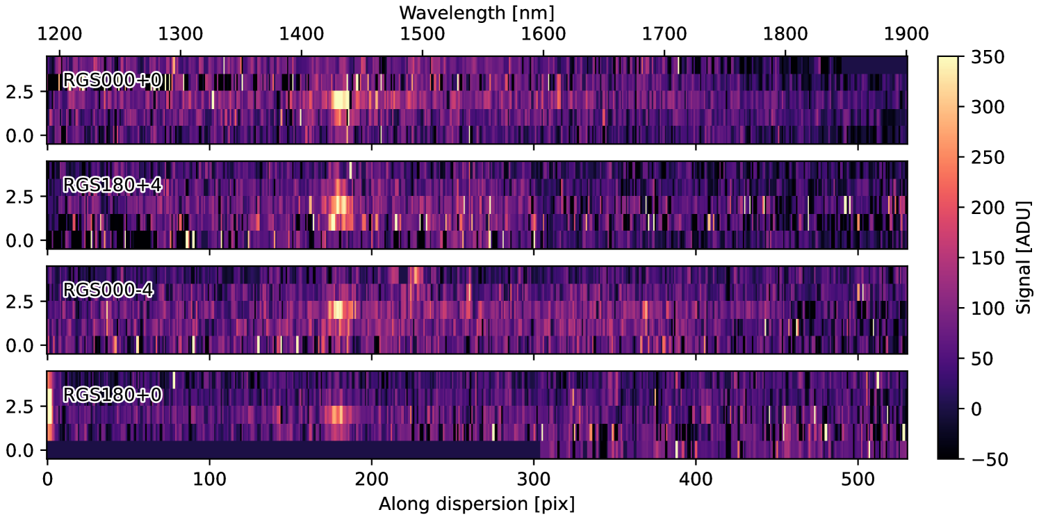
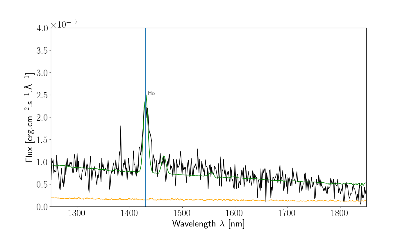
7.5.2 Redshift measurement
The next step is to determine redshifts and measure line fluxes from the extracted spectra, and to provide an estimate of the reliability of the measurements. In the case of EWS observations, the spectra are obtained with the RG, while for the EDFs, the blue grism (BG) spectra are included to enhance the performance of the redshift estimation and to maximise the purity and completeness. Photometric measurements from VIS and NISP could be optionally included and used for the redshift measurement.
The redshift measurement itself is performed through template fitting over a regular grid of redshifts, spaced logarithmically. A first pass uses a coarser logarithmic grid (initial step logarithmic grid, after which a redshift probability density function (PDF) is calculated for each model. All those individual PDFs are combined into one so-called ‘first pass PDF’. A first list of redshift solutions is based on the main peaks (up to 10) of this first PDF. The redshift measurement is then refined around each of these solutions by refitting over all the models, but with a finer redshift grid; the PDF is recalculated and the best final solutions (up to five) and corresponding models are then obtained from the strongest peaks. The peaks are ordered following the value of the integral of the PDF under each peak with a window.
The model includes a set of six distinct continuum models representing various star-formation histories from the Bruzual & Charlot (2003) library. Given the resolution and limited wavelength coverage of NISP, we found that it is not necessary to have more detailed continuum parameters, because it only leads to degeneracies between the different templates. We then add nebular emission lines from templates describing various ratios between the different emission lines. These templates have been built from the more than 35 000 galaxies of the VVDS programme (Le Fèvre et al. 2013), which provides an unbiased sample of spectra for a wide range of galaxy types with , but with magnitude limit of . Using these templates is more efficient than fitting all possible emission lines independently, since the number of free parameters becomes too high to provide a reliable solution. Finally the model includes intrinsic reddening based on Calzetti et al. (2000) and intergalactic medium (IGM) absorption as described in Meiksin (2005).
It is also possible to include priors in the calculation of the PDF, which can be used to favour solutions where a detected emission line is identified as one of the strongest emission lines usually detected in galaxy spectra (e.g. [O II], [O III], H), or just H. Alternatively, one can use the known redshift distribution of H emitters as a baseline for the PDF instead of a flat prior. Tests have shown that such an empirical prior gives the best results in terms of purity and completeness (also see Sect. 7.7.1).
In addition to the galaxy model, the pipeline also provides solutions for quasar and stellar models. The quasar model is built in the same way as was done for galaxies, but including a series of double power-law continuum and Lorentzian broad emission lines. The stellar models are built from a set of 36 templates covering all stellar types (Pickles 1998). The selected object class corresponds to the highest statistical evidence over the three categories (galaxy, star, or quasar).
Once the redshift has been calculated, the fluxes of the detected emission lines are measured using both direct integration (DI) and a Gaussian fit (GF). In the DI method, the spectrum is first continuum-subtracted, using the continuum evaluated from a median-iterate filtering smoothing with a variable window. Each line is then integrated, starting from the position of the peak as provided in the previous step, until the flux remains positive; together with the flux, also the S/N, equivalent width (EW), and position of the lines are provided. In the GF method, a multi-Gaussian model plus a constant continuum model is considered, with Gaussians, depending on the line considered: (i) if a blend with adjacent lines is expected (e.g. we assume three Gaussians for the H+[N ii] doublet complex); or (ii) if the lines are separate but close in wavelength, and their ratios can be linked through physics (e.g. two Gaussians for the [O iii] and [S ii] doublets), or if a line is isolated (e.g. one for H). In contrast to the DI method, this allows for us to deconvolve the contribution of different lines in a complex (e.g. H from [N ii]). This model is used to fit the data with a Levenberg–Marquardt algorithm, deriving the flux, S/N, continuum, FWHM, EW, and wavelength for all the lines, assuming the (up to) five redshift solutions (with their uncertainties) obtained in the step before for each galaxy.
Spectra of objects below redshift 0.9 display very few features in NISP spectra, and hence any artefact in the spectra might be misinterpreted as an emission line. It is therefore essential to identify those spectra that are affected by artefacts: these interlopers could outnumber the targets of the EWS () because the redshift distribution peaks around 0.5 for the limiting AB magnitude of in the EWS. To discriminate objects with secure redshift measurements from possible interlopers, the pipeline provides a numeric indicator of the ‘reliability’ of the redshift measurement, which quantifies the quality of the spectrum based on the analysis of the PDF using a deep-learning algorithm. This algorithm will be trained on EWS-like observations of the EDS, for which a correct redshift at the 99% confidence level is expected. This training will be applied to the set of PDF of the EWS spectra to quantify the reliability of the redshift measurements.
7.6 Measurements for 3×2pt statistics
As discussed in Sect. 2.3 the shape measurements from Euclid are combined with photometric redshifts derived from multi-band photometry. The precise photometric redshifts are required to divide the sample into tomographic bins, while their redshift distributions need to be characterised well for a correct interpretation of the clustering and lensing signals. In Sect. 7.6.1 we describe how the photometric redshifts are determined and we plan to calibrate the corresponding redshift distributions to high accuracy. As described in Sect. 7.6.2, the photometry is also used to classify the objects for further science applications.
The galaxy shape measurements benefit greatly from the sharp diffraction-limited PSF. Nonetheless, our objectives require its size and shape to be determined with unprecedented accuracy. This implies that we have exquisite knowledge of the optical properties of the telescope and understand how the detectors record the incoming photons. This is, however, not sufficient: the PSF is chromatic, which means we need to estimate the appropriate PSF for each galaxy based on its observed SED. This requires a dedicated procedure that is described in Sect. 7.6.3.
The requirements for Euclid were derived by considering the change in the observed unweighted quadrupole moments, , when a galaxy image is convolved by the PSF. For an object with an observed surface-brightness distribution, , and total flux, , its quadrupole moments are defined as
| (20) |
The shape of an object can then be quantified by combining the quadrupole moments into the complex polarisation (or distortion)232323This definition is related to the third flattening (see Sect. 2.2) through . , , where
| (21) |
while the size of an object is captured by
| (22) |
Although unweighted moments are not practical in the presence of noise and blending, they do provide a convenient framework to quantify the impact of the PSF on shape measurement (Paulin-Henriksson et al. 2009; Massey et al. 2013). In this case, the observed quadrupole moments of a galaxy are given by the sum of the quadrupole moments of the true galaxy image and those of the PSF (Valdes et al. 1983), so that
| (23) |
Cropper et al. (2013) used this to allocate tolerances for a wide range of instrumental effects, starting from an acceptable level of bias in cosmological parameters. A limitation of this simple ‘flow down’ is that it did not capture spatial variations of sources of bias, resulting in conservative estimates for the impact of residual systematics on the observed lensing signal (Kitching et al. 2019). To explore a more realistic scenario, Euclid Collaboration: Paykari et al. (2020) considered a ‘flow-up’ from perturbations to the defocus of the PSF model to the bias in cosmological parameters. They found that PSF variations at the level of the requirements induced biases of about 4% of the expected statistical uncertainty in dark energy parameters, well within requirements. Further tests, using simulated data, confirmed that the requirements derived by Cropper et al. (2013) are adequate and conservative and thus remain the basis for the calibration of VIS data (Sect. 4.3) and the modelling of the Euclid PSF, which is described in detail in Sect. 7.6.4. The challenging task of accurate shear estimation from the Euclid images is discussed in Sect. 7.6.5.
7.6.1 Photometric redshift estimation
As shown in Eq. 14, the amplitude of the lensing signal depends on the redshift distribution of the sources, in addition to the cosmological parameters. Moreover, being able to separate the overall galaxy sample into subsamples that are separated in distance enhances the amount of information that can be extracted from a weak lensing, or 3×2pt analysis. The current baseline configuration uses 13 evenly populated bins in the redshift range .
The mean redshift of these subsamples is of particular importance for cosmic shear, since a bias in the estimated mean redshift directly translates into a bias in cosmological parameter inference. Given the objectives of Euclid, this implies that the mean redshift must be known to per bin (Ma et al. 2006; Amara & Réfrégier 2007). Importantly, the modelling of the photometric clustering signal in the 3×2pt analysis relies not only on accurate knowledge of the mean redshift, but also of the width of the redshift distributions of the different subsamples (e.g. Tutusaus et al. 2020; Porredon et al. 2022). The need for precise photometric redshifts is therefore two-fold: to place objects in narrow tomographic redshift intervals, minimising the overlap between subsamples; and to ensure that the distribution in redshift of the sources in each subsample is accurately known. These two needs are addressed separately in the photometric redshift pipeline, since the former requires that we optimise the photo- for precision, while the latter demands very high accuracy.
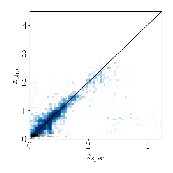
For individual galaxies, the need to place objects in tight redshift intervals, with being a key requirement, leads to two considerations: the effective dispersion of the PDF around its assumed true redshift (‘photo- scatter’); and the probability that our assumed redshift for an object is far from its true redshift (‘outlier rate’). Further requirements are placed on the choice of the photo- algorithm by the nature of the EWS. It must be able to run efficiently for the billions of galaxies we will observe and to be able to account for effects that vary on an object-by-object basis, namely the impact of Galactic reddening and the variation of filter transmission curves across the FoV of an instrument (Euclid Collaboration: Paltani et al. 2024). These additional concerns led to the development of the NNPZ (Nearest-Neighbour Photometric Redshifts) algorithm; its performance on a sample of spectroscopic redshifts taken from the COSMOS field is shown in Fig. 30. These results were taken from the Euclid photo- data challenge of Euclid Collaboration: Desprez et al. (2020), which compared different methods using simulated DES (optical) and Euclid (NIR) data. The photometric redshift quantity that is used to assign tomographic redshift bins is the mode of the NNPZ PDF, and for the sample shown in Fig. 30 the scatter () and outlier fraction () of this photo- with respect to the spectroscopic redshifts lie slightly outside of our requirements ( and , respectively). This is adequate for the first data release (DR1; see Sect. 7.8), while we expect to achieve a better performance for later releases, once much deeper LSST data become available.
Machine-learning algorithms such as NNPZ rely heavily on how representative the reference training data are of the target data set. Complete and representative spectroscopic samples are impractical to assemble for the EWS, and so instead we will build a sample of galaxies with accurate and precise photometric redshift PDFs from a carefully selected and curated set of deep reference fields, the EAFs. These reference field photo-s will be computed using a new custom SED-fitting package called Phosphoros (see Sect. 3.3 in Euclid Collaboration: Desprez et al. 2020, for a brief description). Through tagging the SEDs with properties, such as a mass-to-light ratio or metallicity, Phosphoros is able to additionally produce sampled posterior distributions of physical quantities (e.g. stellar masses) for each reference galaxy. The PDF and multi-dimensional physical-property posterior information can then be propagated from these reference field galaxies to the EWS galaxies with NNPZ. In this sense, NNPZ operates as an accelerator for the template-fitting approach, and its lack of an explicit training phase allows us to account for effects that vary on an object-by-object basis (Euclid Collaboration: Paltani et al. 2024). The PDFs we output at this stage are still expected to be subject to biases, due to our imperfect knowledge of galaxy SEDs and the priors we use, and are therefore used only for tomographic redshift binning in the weak lensing analysis. The galaxy physical properties inferred through this process are not used in the weak gravitational lensing analyses, but will be used for a vast range of non-cosmological applications (see Sect. 10).
Once galaxies have been assigned to their tomographic redshift samples, we must reconstruct their collective distribution in redshift, , for cosmological inference of the weak lensing signal. The strategy to achieve the target accuracy of per tomographic bin was outlined in Masters et al. (2015) and has evolved only a little since then. Briefly, the 8- or 9-band photometric space of the target galaxy sample is quantised by way of a SOM (Kohonen & Honkela 2007), resulting in a 2-dimensional array of vertices or ‘cells’ (also see Fig. 19). Each cell of the SOM is represented by a vector of values, where each value corresponds to the ratio of flux in a photometric band with respect to the value, and thus each cell represents a possible galaxy SED with free amplitude. Galaxies in the weak lensing sample are each assigned to their closest SOM cell in the flux-ratio space used to construct the SOM. The SOM algorithm preserves locality of the input space, in the sense that similar vectors of flux ratios with respect to will be nearby to one another in the 2-dimensional SOM map, and therefore each cell has a finite size in the input parameter space. The Euclid survey is supported by ground-based observations with different instruments and filters for the northern and southern regions (see Sect. 4.4). To place all galaxies correctly in the SOM we perform a band-standardisation step whereby a per-galaxy colour term is computed and applied to the observed photometry in each band. Corrections for Galactic reddening and bandpass variation are also carried out during this step.
Construction of the is based on the spectroscopic sample built up through the C3R2 programme (see Sect. 4.5). The sample is designed to cover the diversity of galaxy SEDs in the shear sample, but the measured SED of an object depends on the noise properties of the observations and other survey characteristics. In order to be able to account for varying survey depth, the spectroscopic sample is drawn from the EAFs (Sect. 4.2.2), where the of the data are five times higher than the EWS. We can then draw multiple realisations of the EWS noise properties and apply them to these objects to form a calibration sample that covers both the range in galaxy SEDs and photometric scatter of the shear sample.
With the calibration sample in hand we perform the estimation for each tomographic redshift subsample separately. Each galaxy in a subsample is assigned to its best-matching SOM cell and the shear weights of objects (see Sect. 7.6.5) are summed within each SOM cell. These sums of weights represent the statistical power of each SOM cell, with an analogous quantity determined by each objects’ probability to pass the selection flux cut in the case of photometric clustering. The calibration objects are treated in the same way, with the exception that their ‘shear weights’ are always unity, that is, their PDFs are measured via NNPZ and their artificially noised flux measurements are dereddened and band-standardised in the same way as for the shear sample. The calibration objects are then assigned to tomographic bins on the basis of the mode of the PDF, exactly as for the shear sample objects. They are also rendered into the SOM and the number of them per SOM cell, within the given tomographic bin, is computed. The redshift distribution of a tomographic bin is then just a weighted histogram of the spectroscopic redshifts, where the weight of a spectroscopic object is the sum of shear weights in its cell, divided by the number of spectroscopic objects in that cell. In this way, all trusted redshifts per cell are used, but the relative sampling difference between the shear sample and the selection of objects for which we have spectroscopic redshifts is accounted for.
There are some SOM cells containing galaxies that can be used for the weak lensing analysis, but that lack spectroscopic measurements. Those galaxies are flagged and removed from the analysis because we are unable to represent them in the recovered redshift distribution. With this strategy, the distribution is subject to sample noise, but Masters et al. (2015) showed that we will be able to meet our target requirement of on the mean redshift per tomographic bin, provided that each tomographic subsample is represented by a large () number of cells.
As a further validation of the redshift distributions estimated with the SOM method, we will use clustering redshifts (Newman 2008). This method employs angular cross-correlation measurements of the positions of the sources in the tomographic bins and spectroscopic calibration samples that overlap on the sky. Crucially, this drops the assumption of the calibration sample fully covering the colour and magnitude range of the source sample. As such, different calibration samples that are typically brighter and cover larger areas are used, which makes this approach highly complementary to the SOM method. Measuring the angular cross-correlation amplitude between the tomographic source samples and the spectroscopic calibration samples finely binned in redshift can result in an accurate reconstruction of the tomographic redshift distributions. As shown in Naidoo et al. (2023), an overlap area of only a few hundred square degrees between the Euclid source sample and spectroscopic surveys like BOSS, DESI, and the Euclid NISP-S sample is sufficient to reach the requirement on the accuracy of the mean redshift of the tomographic bins.
7.6.2 Classification
The objects detected in Euclid images comprise galaxies, stars, QSOs, globular clusters, Solar System objects, and a diverse array of contaminants and artefacts. In order to avoid introducing selection effects in the weak gravitational lensing analysis, each detected object with a full complement of photometric information available is treated as a possible galaxy at the photometric redshift determination stage. Contaminants and stars are determined during the shape measurement process (see Sect. 7.6.5) by their low shear weights. However, to facilitate the modelling of the PSF we must identify a very pure sample of stars that spans the range of stellar colours. Using only morphological information, such as an object’s apparent compactness, risks introducing biases into the PSF model, and so this step is ideally performed using only photometric information.
Our classification uses a set of three pretrained probabilistic random forests (pRFs), each a binary classifier for a type of object, such as star versus not a star. The pRF returns a probability that an object is of that type and thus each object receives three probabilities, one for each of the considered types, namely star, galaxy, and QSO. An object is assigned a given class if its probability to be that class exceeds a predetermined threshold, and a single object can be given multiple classes. Only those objects classed as stars and not any other additional classes are considered suitable for PSF modelling. Class probabilities are retained for use in non-cosmological legacy science processing (see Sect. 10).
7.6.3 SED modelling
The convolution of galaxy images by the PSF is the dominant source of bias for weak lensing studies, and an accurate estimate of the PSF is required to obtain unbiased shape measurements. Here, we focus on the challenges that arise from the fact that the Euclid telescope is diffraction limited and the VIS passband is very broad (see Cypriano et al. 2010; Eriksen & Hoekstra 2018, for more background). In the analysis we need to take into account that each galaxy is convolved by an effective PSF that depends on its SED. Moreover, to determine the underlying optical PSF model successfully, we must know the SED of each of the stars that is used in this process.
For bright stars () Gaia spectra can be used directly, but for fainter objects we must estimate their SEDs at high accuracy from their broad-band photometry (Eriksen & Hoekstra 2018). To perform this task we re-use NNPZ, the nearest-neighbour method that was developed for the main photometric redshift pipeline, but choose as target quantities the fluxes at different wavelengths. Similar to what is done to determine the redshift probability density functions (PDFs), we construct a reference data set of objects that is in principle representative of the objects for which we need to recover the SED information. Specifically, we use the Gaia spectra, assuming that across the Euclid footprint we have examples of all relevant stellar types and metallicities. An analysis of the impact of differential Galactic reddening between brighter and fainter stars of the same types (and thus different radial distances) is ongoing. We integrate the Gaia spectra through a series of 55 synthetic narrow-band filters of width 10 nm, filling the range , and recover the weighted mean flux from the closest neighbours. The weight is a pseudo-likelihood computed from the distance in flux space between the target object and a reference object, with a free SED amplitude parameter.
The measurement of galaxy SEDs follows a similar procedure, but in this case we lack an equivalent to the Gaia spectro-photometric data set. Moreover, existing sets of galaxy SED templates are either incomplete or biased and would thus introduce biases in the PSF construction that would propagate to cosmological parameter estimation (see Eriksen & Hoekstra 2018).
The strategy to create the NNPZ reference sample for galaxy SEDs is summarised as follows. Instead of using spectra, we begin with broad- and intermediate-band photometry from the COSMOS and CDFS fields to provide a coarse sampling of galaxy SEDs through much of the bandpass range. We then apply a combination of Gaussian process (GP) interpolation and template-guided filter colour terms to achieve the finer 55 narrow-band sampling that we also use for the stellar SEDs. To reduce the impact of sample variance we plan to collect additional medium band data across the EAFs.
7.6.4 VIS PSF model
As discussed in detail in Cropper et al. (2013), accurate measurement of weak lensing shear imposes stringent requirements on model accuracy for the Euclid VIS PSF. In the case of Euclid, this means that the PSF model must be known throughout the mission lifetime with a residual temporal-spatial model uncertainty of per ellipticity component, while the size needs to be known such that . Although the Euclid VIS system possesses a highly stable, diffraction-limited PSF, meeting these requirements is nonetheless challenging because of a number of design choices.
First, to reach the required depth, VIS uses a broad bandpass, but this also results in a strong chromatic dependence for the PSF. Hence, as already discussed in Sect. 7.6.3, the PSF varies between stars and galaxies according to their colour or SED, and within galaxies due to local changes in stellar populations (i.e. colour gradients within galaxies; Semboloni et al. 2013a; Er et al. 2018). Moreover, Euclid utilises a dichroic to split the visible and NIR components of the beam, which was designed to produce a hard bandpass edge with minimal out-of-band light (in conjunction with coatings also applied to two of the fold mirrors). This is achieved using a complex multi-layer dielectric coating, which induces wavelength- and polarisation-dependent phase errors on the wavefront and consequent effects in the PSF model (Gaspar Venancio et al. 2016). This is further influenced by chromatic, polarised reflection from the silver optical surfaces and fold mirror coatings, and transmission at the detector. Finally, the pixel size of the Euclid VIS CCDs is such that the PSF is undersampled at all wavelengths in the VIS bandpass.
Hence, in addition to capturing the variation across the FoV, the VIS PSF model also needs to allow for the propagation of the model between stars and galaxies with differing SEDs. Together with the need to produce an oversampled model, to address pixel undersampling, this motivates utilising a PSF forward-modelling approach. The Fraunhofer condition links the image-plane PSF to the wavefront error at the exit pupil of the telescope (e.g. Hopkins & Yzuel 1970). Under this condition, one may forward model the PSF on the detector FPA using a combination of chromatic wavefront modelling for the optical contributions and both chromatic and achromatic convolutional kernels for the detector and guiding error contributions (also see Ma et al. 2008). When modelling the PSF, it is essential to analyse image data that have had all linear and nonlinear detector effects corrected, including detector nonlinearity and the brighter-fatter effect (BFE), the latter currently being corrected by a modified version of the algorithm due to Coulton et al. (2018).
An important benefit of forward modelling is that a wide range of effects can be included in a consistent fashion. In the case of the VIS PSF model, these include the following.
-
•
A model for vignetting of the pupil by the secondary optics structure, constructed from industry-supplied CODE V242424CODE V® is a commercial optical design tool. model inputs and tested against CODE V model outputs.
-
•
Optical path differences due to optical layout, modelled locally on the pupil plane as a weighted sum of Zernike polynomials. Zernike polynomials are a natural basis set for this contribution, since they are defined to be orthogonal on a circular pupil, although the vignetting breaks the orthogonality of the polynomial set in this application. Variation across the FPA is included as a polynomial fit across the FoV for each Zernike polynomial.
-
•
The surface figure error (SFE) contribution to the wavefront error, resulting from imperfections of each reflecting surface, are included by propagating a model for the beam footprint on pre-launch measured SFE maps for each optical surface.
- •
-
•
Detector charge diffusion is modelled as in Niemi et al. (2015), as a chromatic convolutional effect.
-
•
Chromatic dependencies, including polarisation-dependent telescope throughput, detector quantum efficiency, and source SEDs, are included as spectral weightings in the broadband, chromatic PSF model, which is computed by spline interpolation of monochromatic calculations at multiple wavelengths, followed by integration across the VIS passband and out-of-band optical wavelength region.
-
•
The chromatic response to polarisation from mirror coatings, most notably the layered dielectric coatings of the dichroic, the silver coating on FOM 3, the coatings on FOM 1 and 2 at high angles of incident light, and the hafnium oxide coating on the detector. In particular, the layered dichroic coating induces a strong chromatic and FoV dependence, which must be accounted for in the model. To characterise this dependence and to provide inputs for the PSF modelling, we have commenced an extensive test campaign on the spare model of the dichroic (Baron et al. 2022, 2023; Baron 2024). The polarisation dependence of the VIS optical system is modelled following Chipman et al. (2019, chapters 11,16). An FoV- and wavelength-dependent set of four ‘Jones pupils’ is produced from the CODE V model of the optical surfaces and layout. The Jones pupils describe the system’s polarised response to orthogonal input polarisation states across the pupil. They are included in the construction of the complex electric field at the exit pupil, and transformed to the monochromatic PSF at a given wavelength for a given set of Stokes parameters, via the construction of an ‘amplitude response matrix’ and Mueller point-spread matrix. We emphasise that this effect must be included even for unpolarised incident light, which should be considered as a combination of two incoherent orthogonal polarisation states.
- •
The wavefront model for the Euclid VIS PSF allows for a fully flexible and modular parameterisation, including chromatic, spatial, and temporal variations. The SFE, dichroic, and detector contributions, with the exception of CTI, are expected to be invariant across the mission lifetime and therefore the models for these are fixed using laboratory measurements. The telescope pointing stability is measured during observations using the FGS, and propagated to the model for any given exposure. However, the optical model is expected to vary throughout the mission, due to thermal variations arising from changing telescope orientation with respect to the Sun and due to variations in spacecraft heat inputs. Distortions to the telescope structure under gravity and perturbations resulting from the launch process mean that laboratory measurements of the optical alignment cannot predict wavefront errors, and instead these must be inferred from in-orbit data.
The PSF model is therefore calibrated across the lifetime of the survey using a hierarchical calibration process consisting of three steps. First, the initial state of the PSF model is inferred from PV (Sect. 4.3.1) and early science operations (ESOP) data across a range of spacecraft attitudes with respect to the Sun vector. This is used to produce a basis set of spatially dependent PSF variations, which can be fit to further observations at other attitudes. Since PSF optical modes are expected to be degenerate with detector modes (e.g. the charge diffusion kernel), this process is conducted iteratively, alongside fits for detector modes, until requirements on validation metrics are met. Because detector modes are not expected to vary across PV and ESOP calibration data, they are fit in a meta-analysis of the full calibration data set. This basis set is then updated from continuous observations with a monthly cadence, and any perturbations to the basis set modes are fed through to further optimisation. The monthly calibrations are taken on a limited set of defined fields, to simplify the interpretation of PSF variations between observations. This process should capture long-timescale variations. Finally, the resulting calibrated basis set is fit to each science observation, producing short-timescale variation on the timescale of science observation cadence. This enables an accurate PSF model to be produced for shear measurement in each science observation.
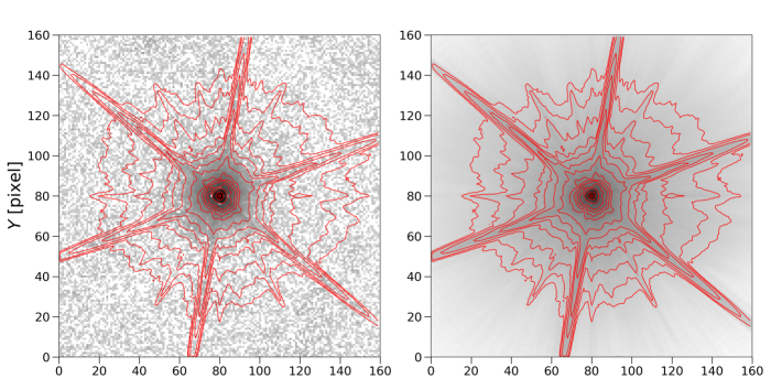
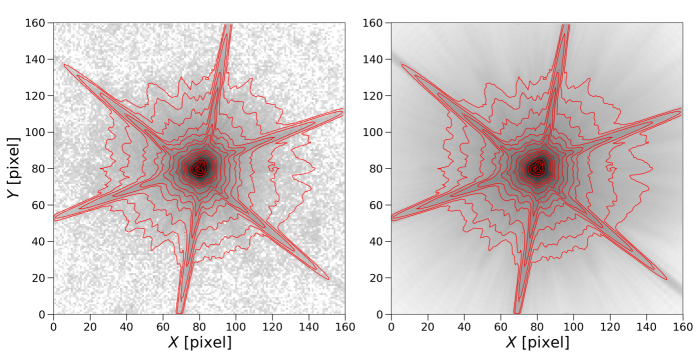
In the calibration, the initial telescope optical state is assumed to be maximally unknown, whereas the PSF model contains degenerate effects, both between optical Zernike modes and between detector and guiding error effects. Together, this can make it difficult for initial PSF calibration to robustly determine the underlying optical parameters that are used to infer the PSF across the mission lifetime.
We therefore utilise phase-diverse observations to calibrate the PSF model during the observation of PV and ESOP calibration images (see section 4.3.2). The phase diversity technique (e.g. Gonsalves 1982; Fienup 1982) adds known aberration to the observations, and for the Euclid mission we add defocus by deliberate movement of the M2 mirror along the beam propagation direction. Adding a known defocus serves two purposes: first, it causes optical modes to become distinct from detector modes, due to dispersion of the PSF across a wider scale of pixels; and second, perturbations in optical modes induce differing impacts on the PSF image for each defocus, allowing a joint fit that lifts degeneracies between optical modes. Together, the phase-diverse calibration allows for the model parameter optimisation to robustly find the true best-fit model parameters, by simplifying the posterior that is optimised, through lifting degeneracy and multi-modality. These phase-diverse data are analysed with a model-fitting approach, to account for the wide VIS passband and the image undersampling (cf. Fienup 1999).
Figure 31 shows the pre-calibration VIS PSF model, fit to a PDC test data set taken during the PV phase. This comprised three sets of 10 exposures, taken at nominal in-focus and with two defocus offsets, applied as a movement of the M2 mirror by m, corresponding to about 0.8 waves of defocus. Larger defocus amounts are prohibited by the requirement to operate the FGS. Also shown are stacked profiles of stars in that data set, applying pixel-level sigma-clipping to remove contaminating sources. This stacking procedure was carried out on both the stars and the model images fit to those stars. Red contours show isophotes for the model PSF. We see that the features of the PSF, as observed in the stars selected in the data, are well described by the PSF model. There is good agreement on all scales, including in the wings of the PSF, with good alignment of the diffraction spikes caused by the spiders holding the M2 mirror, including lateral translation of those spikes in the defocused images, and the halo caused by SFE on M1. We note that these models were fit to a set of phase-diverse test data with approximately 15 times fewer exposures than the PV and ESOP PDC calibration sets, and the models shown are not yet expected to satisfy the model accuracy requirements discussed above.
7.6.5 Shape measurement
Although Euclid is designed to provide sharp images of distant galaxies, the observed shapes are biased because of the convolution with the PSF, noise in the images, blending with other galaxies, the presence of cosmic rays, as well as a variety of detector-related sources of bias. These amount to biases that dwarf the lensing signal itself, and thus all need to be carefully accounted for.
Over the years much effort has been spent on developing and testing methods that aim to provide accurate ellipticities for individual galaxies (see e.g. Heymans et al. 2006; Massey et al. 2007; Bridle et al. 2010; Kitching et al. 2012a, 2013, b; Mandelbaum et al. 2015, for the results from several community-wide efforts). The sensitivity of algorithms to certain systematics will differ, and hence it is advantageous to consider several approaches. A well established method is to fit parameterised models to the observed surface brightness. To this end, we have developed LensMC (Euclid Collaboration: Congedo et al. 2024), which is based on forward modelling galaxies with fast Markov chain Monte Carlo (MCMC) sampling and marginalisation over nuisance parameters. It measures the properties of objects from the multiple exposures jointly, while mitigating the bias due to detected neighbours by measuring objects in groups. The robustness has been proven on realistic simulations of EWS images, using galaxies drawn from the EFS as input. The development of LensMC has benefited from the knowledge gained from the ground with lensfit (Miller et al. 2007; Kitching et al. 2008a; Miller et al. 2013), which has been successfully applied to the various data releases of KiDS (e.g. Fenech Conti et al. 2017; Kannawadi et al. 2019; Li et al. 2023a).
An alternative route uses the observed moments of the surface brightness. For instance, MomentsML (Tewes et al. 2019) is a machine-learning algorithm that trains a neural network to estimate the shape parameters from the moments of the surface-brightness profiles of galaxy images. In principle, this can reach the required accuracy, but it does rely critically on the realism of the simulated training data. This is a general concern for shape measurement (e.g. Hoekstra et al. 2017; Kannawadi et al. 2019), also because biases are already introduced during the object detection stage (e.g. Fenech Conti et al. 2017; Hoekstra et al. 2021). To (partially) circumvent these concerns, MetaCal (Sheldon & Huff 2017; Huff & Mandelbaum 2017) measures the shear response of an object for any shape measurement method by directly distorting its observed images. It has already been extensively applied to the DES lensing analysis (Zuntz et al. 2018; Gatti et al. 2021). Moreover, tests on realistic simulated images have shown its potential for Euclid (Hoekstra 2021; Kannawadi et al. 2021; Hoekstra et al. 2021). Hence, work is ongoing to develop a MetaCal setup for the analysis of Euclid data.
Simulated images are also needed to calibrate the biases introduced by other complications, such as the blending of galaxies at different redshifts (MacCrann et al. 2022; Li et al. 2023a) or specific detector effects. The latter includes the non-uniformity of the pixel response over the CCD, bleeding due to charge overflow in a pixel, and CTI in the readout process. Other effects that need to be quantified are the various sources of background noise, variation in the star density, cosmic rays, galaxy blending, and contribution of unresolved galaxies to the background (Euclid Collaboration: Martinet et al. 2019). Many of these effects only become relevant because of the precision that Euclid can achieve. Some are very specific to space-based observations where radiation damage leads to CTI. The impact on the VIS images can be modelled following Massey et al. (2014), All these effects must be accurately included in the simulation pipeline described in Sect. 6.2 to reach a successful calibration (e.g. Hoekstra et al. 2015, 2017).
As already discussed in Sect. 2.2, the shear biases can be split into a multiplicative and additive contribution (see Eq. 17), assuming the applied shear in the simulations is sufficiently small, or the algorithm sufficiently linear. In some cases it can be useful to isolate PSF leakage from the additive bias, adding the term to Eq. 17, where quantifies the imperfect correction for the PSF ellipticity .
Massey et al. (2013) showed that to reach our scientific goals (also see Sect. 2), the uncertainties in the multiplicative and additive shear bias must remain below and , respectively, for each component of the shear. These numbers represent the total error budget, which then needs to be divided among several contributions (Cropper et al. 2013). Reaching such accuracy on shear measurement requires calibrating on realistic image simulations over a wide enough area so that measurement errors on these biases are negligible compared to the target accuracy. The required number of simulated galaxies, , to reach a given uncertainty in the total multiplicative shear bias, , is given by (Fenech Conti et al. 2017; Euclid Collaboration: Congedo et al. 2024)
| (24) |
where is the modulus of the shear applied to the simulated galaxies,252525The simulations may use a different shear for each galaxy to capture the impact of the blending of galaxies at different redshifts (MacCrann et al. 2022; Li et al. 2023a) or a constant shear across the entire scene (Kannawadi et al. 2019; Li et al. 2023a, e.g.) and is the dispersion of intrinsic ellipticities, taken to be in the case of Euclid (Euclid Collaboration: Martinet et al. 2019). However, this number can be lowered by shape (Massey et al. 2007) and pixel (Euclid Collaboration: Martinet et al. 2019) noise cancellation. In the former, pairs of galaxies with rotation are considered, so that the mean intrinsic ellipticity reaches in the absence of noise, and in the latter an extra identical pair with noise of opposite sign is included to lower the impact of shot noise in the calibration process. Together, these cancellations improve the runtime of the calibration simulations by a factor of 7 in the case of Euclid (Jansen et al. 2024).
Since galaxy morphologies depend on redshift, the calibration must be performed for each tomographic bin to avoid any undesired selection effects (e.g. Kannawadi et al. 2019). This process multiplies the number of nuisance parameters related to the calibration that need to be passed to the likelihood by the chosen number of tomographic slices. It also means that the shear and photometric redshift calibration must be performed jointly and that the galaxy morphology and photometry dependence on redshift must be accurately reproduced in the calibration simulations (Li et al. 2023a). Finally, the chromaticity of the VIS PSF, combined with the SED variation across galaxy bulges and disks, introduces a non-negligible residual bias in shear measurements. This effect is referred to as ‘colour gradient’ bias (Voigt et al. 2012). Semboloni et al. (2013a) showed that it is possible to correct for it on average using estimates for the bias from HST imaging in two narrow filters (F606W and F814W), which has been confirmed to be sufficient for Euclid by Er et al. (2018).
7.7 Science-ready data products
The carefully calibrated data products that have been described in the previous sections can be used for scientific exploitation. The enhanced galaxy catalogues contain information about the redshifts and stellar masses of galaxies, as well as detailed morphological information and extensive photometry in all bands. To enable the various cosmological analyses, however, the catalogues are processed further. The cosmological information contained in the catalogues is compressed into the various two-point statistics that have been introduced in Sect. 2. In Sect. 7.7.1 we summarise the steps in the calculation of the clustering statistics of the spectroscopic clustering sample, while Sect. 7.7.2 describes the summary statistics needed for the 3×2pt analysis. Moreover, high-resolution maps of the projected mass distribution (Sect. 7.7.3) and a catalogue of clusters of galaxies with a well defined selection function (Sect. 7.7.4) are provided.
7.7.1 Spectroscopic clustering statistics
As discussed in Sect. 2.1, the statistical properties of the galaxy distribution can be quantified in terms of a set of clustering moments, which compress the cosmological and astrophysical information from galaxy surveys. The most fundamental measures of galaxy clustering are two-point statistics, which fully characterise the fluctuations in a Gaussian density field.
The starting point is the spectroscopic galaxy catalogue, described in Sect. 7.5. Since the spectroscopic measurements are made with a slitless spectrograph, it is necessary to apply a selection process to identify the galaxy sample with confident redshift measurements. The EWS will be primarily sensitive to luminous emission line galaxies in the redshift range with an H line flux above the nominal limit of . The catalogue will be selected to maximise the galaxy number density, while keeping the fraction of spurious redshift measurements under control. It is important to account for potential systematic effects that can modulate the detection limit and remove genuine galaxies from the sample, or lead to errors in the redshift measurement that add interloper galaxies and reduce the purity. These inaccuracies in the selection have a direct impact on clustering statistics.
The redshift purity and completeness of the sample will be evaluated using the EDFs (Sect. 4.2.1), which enable a detailed assessment of the spectroscopic selection function across the EWS. The selection function will be characterised by a random catalogue of mock, unclustered objects that is constructed to closely trace the mean density of galaxies in the EWS and exhibit the same angular and radial selection effects. Constructing this random catalogue involves a forward-modelling process that relies on the noise level estimated in the NISP exposures and approximate end-to-end simulations of the spectroscopic measurement pipeline.
The resulting selected galaxy catalogue, and its corresponding random catalogue, are provided as data products. Their ‘reconstructed’ versions are also provided; they are obtained by applying a nonlinear transformation to the observed positions of the galaxies aimed at reducing the effect of the nonlinear evolution of cosmic structures and to enhance signal-to-noise on mildly nonlinear scales. Reconstructions can be performed either using the standard Zeldovich approximation approach (e.g. Padmanabhan et al. 2012) or with an efficient implementation of the cosmological least-action method (Sarpa et al. 2021), both of which provide excellent results at the BAO scale.
Original and reconstructed catalogues are used to compute the clustering statistics. The clustering moments can either be measured in configuration or Fourier space, and while they are theoretically equivalent, in practice their estimation can lead to different types of uncertainties and they can be differently impacted by systematic effects. To ensure accuracy, it is important to measure them in both spaces. In configuration space, we measure the spatial 2PCF of galaxies, which quantifies the excess probability of finding two objects at a given separation in a discrete sample of mass tracers with respect to a random Poisson sample. Estimating this quantity involves counting pairs, which can be computationally intensive. Therefore, we prioritise minimising memory allocation and maximising computational efficiency in our implementation of the estimator, while ensuring accuracy within sub-percent requirements.
Apparent deviations from statistical isotropy in clustering measurements depend on the geometry of the Universe and the growth rate of cosmic structures, breaking the circular symmetry of iso-correlation contours. To quantify these effects accurately, our estimator accounts for deviations by decomposing pair separation vectors into polar or Cartesian coordinate systems, which define the transverse and parallel components to the LoS within a local plane-parallel approximation. To achieve computational efficiency and minimise redundancy, we implement two parallel pair-counting algorithms, namely ‘chain-mesh’ and ‘kd-tree’ techniques, both exact in counting all object pairs within a predefined separation range and with varying performance levels in CPU time and memory usage at different scales (Marulli et al. 2016). Our estimator also incorporates the random-splitting technique to enhance computational speed (Keihänen et al. 2019) in the validation tests. This technique involves splitting the random sample, which typically contributes significantly to the computational load, into smaller subsets. The number of subsets can be determined by the user, finding a balance between computational efficiency and accuracy needs. The outputs of our estimator include the first five Legendre multipole moments, see Eq. 9, of the 2PCF, the anisotropic, 2-dimensional 2PCF in polar and Cartesian coordinates, the projected 2PCF, and data and random pair counts. Depending on the option selected by the user, the estimator computes the auto-correlation function of the objects in the catalogue or the cross-correlation of the objects in two different catalogues. Finally, the 2PCF s of the original and of the Zeldovich reconstructed catalogues will be computed.
Various effects render the observed distribution of galaxies non-Gaussian and thus transfer information to higher clustering moments. In order to enable extraction of that information, Euclid will additionally produce measurements of three-point statistics. In particular, we have developed an efficient estimator for the three-point correlation function (3PCF), which employs both the local spherical harmonics approximation technique proposed by Slepian & Eisenstein (2015) and the brute-force triplet-counting approach, which is mainly used for verification purposes. The three-point estimator takes the same input as the two-point estimator, but produces different outputs, namely the connected and reduced 3PCFs for all triangle configurations, as well as the corresponding data and random triplet counts.
The Fourier-space analogue of the two- and three-point correlation functions are the power spectrum and bispectrum, respectively. Their implementation within Euclid follows the methodology of the standard Feldman–Kaiser–Peacock (FKP; Feldman et al. 1994) estimator, which measures correlations of Fourier modes from a weighted fluctuation field. This field is constructed from the difference between the galaxy and random catalogues (see paragraph above), multiplied by weights, which are chosen such that they minimise the variance of the estimator and depend on the number density of the selected galaxy sample. The fluctuation field is then smoothed onto a regular grid that is sufficiently large to encompass the full galaxy catalogue, which enables the use of fast Fourier transforms (FFTs).
In the presence of RSDs, the clustering moments acquire a dependence on the LoS towards a given pair or triplet of galaxies. Measurements of the power spectrum and bispectrum must appropriately account for the variation of the LoS over the extent of the survey footprint, which led Yamamoto et al. (2006) to derive an extension of the FKP estimator (see also Szalay et al. 1998; Yoo & Seljak 2015; Scoccimarro 2015). However, since the Yamamoto estimator presents a computational challenge for data sets as large as those produced by Euclid, in practice one approximates the LoS by that of one of the galaxies in the pair or triplet. With this approximation it is still possible to extract the anisotropic signal using FFTs (Scoccimarro 2015; Bianchi et al. 2015), making the computation efficient, while consequences of this choice of LoS can be addressed at the level of the theoretical models (e.g. Beutler et al. 2019). The implementation for Euclid allows us to measure the first five Legendre multipoles of the power spectrum, Eq. 10, in addition to the monopole, quadrupole, and hexadecapole of the bispectrum.
The clustering two-point statistics moments estimated in Fourier space carry the imprint of the survey selection function (also called the survey window function), which must be accounted for when fitting theoretical models to the measurements. The required correction of the theoretical templates can be computed from the power spectrum of the random catalogue, which is therefore a separate data product of the Euclid pipeline.
7.7.2 Photometric 3×2pt statistics
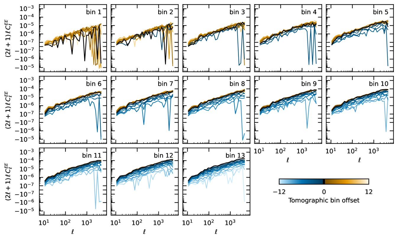
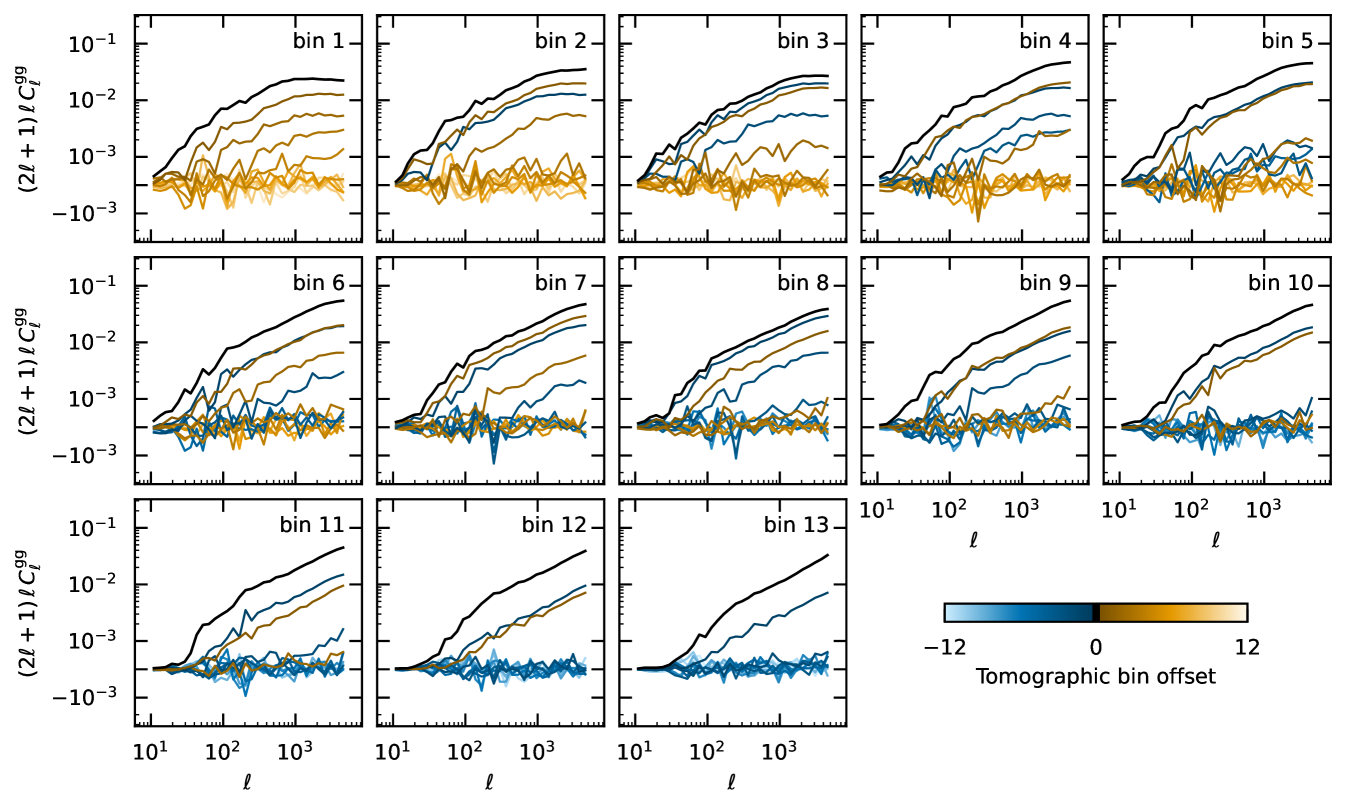
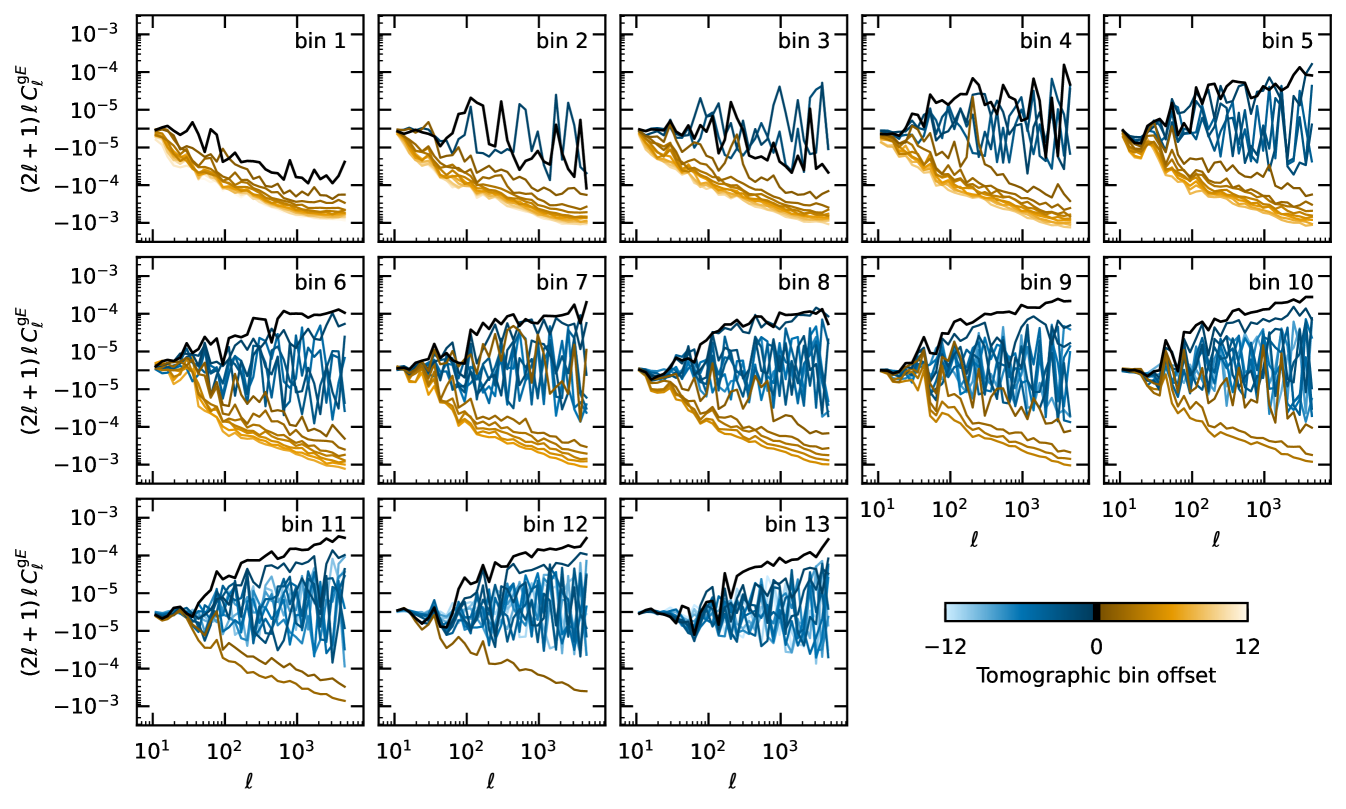
Euclids photometric galaxy samples are determined by their detection in the filter. Nominally, this includes all galaxies with (, extended source) and with valid photometry in all NIR and all available ground-based bands. The resulting samples and their key properties, such as number density and redshift distributions, are further modulated by statistical weights, which typically correlate strongly with S/N in . Data processing enables the full galaxy sample to be split into up to 13 tomographic bins (Euclid Collaboration: Pocino et al. 2021) via point estimates for the photometric redshifts. The bin boundaries will be placed such that the statistical constraining power is optimised (see e.g. Zuntz et al. 2021; Euclid Collaboration: Pocino et al. 2021), while also keeping systematic trends and cross-correlation in the redshift distribution calibration to a minimum.
The galaxy samples used for shear measurement and for photometric galaxy clustering will generally differ, due to different statistical weights and the number and placement of tomographic bins, as well as potentially brighter cuts in to reduce spurious clustering patterns caused by spatially varying selection effects. These selection effects are not only caused by systematic variations in the detection efficiency, such as background noise level, foreground stellar density, or Galactic extinction, but also by trends in all bands entering the photometric redshift estimation, including those from ground-based surveys. This makes it challenging to predict or simulate the full complement of selection effects. By default, we will therefore apply a data-driven approach that learns systematic galaxy density variations from the observed data, closely following methods applied to current imaging surveys (Johnston et al. 2021; Rodr´ıguez-Monroy et al. 2022). Thus, we will construct visibility maps and, equivalently, random catalogues for each tomographic bin in the photometric galaxy clustering sample.
As discussed in Sects. 2.2 and 2.3, we will extract cosmological information from the 3×2pt statistics of the photometric galaxy catalogue. To do so, we measure the two-point correlations of:
-
1.
galaxy ellipticities, tracing cosmic shear;
-
2.
galaxy positions, tracing angular galaxy clustering; and
-
3.
cross-correlations between galaxy positions and ellipticities, tracing galaxy-galaxy lensing.
The 3×2pt statistics are angular statistics, which are measured in projection on the sphere. To obtain information from the cosmological evolution of the galaxy sample, the 3×2pt statistics are computed for all auto- and cross-correlations of the full set of tomographic redshift bins.
We can measure angular statistics on the sphere either in real space, as observed, or in harmonic space, after a spherical harmonic transform of the observations. To maximise the scientific return of Euclid, we will measure the 3×2pt statistics in both real and harmonic space. While there is a mathematical relation such as Eq. 12 for each angular correlation function and its power spectrum, the transformation between real and harmonic space requires information on all angular scales, from the full sky to the infinitesimally small. In practice, we therefore cannot exactly transform one measured statistic into the other, even if both ultimately probe the same information, and we will hence measure them separately.
The main real-space measurement consists of the following estimates of the 3×2pt angular correlation functions:
-
1.
the cosmic shear estimator is a weighted average of the observed shears (Schneider et al. 2002a);
- 2.
- 3.
Each real-space estimate is computed in linear or logarithmic bins of angular separation , and for all combinations of tomographic redshift bins. A secondary set of derived two-point statistics is also measured, consisting of band-power spectra (Schneider et al. 2002a) and Complete Orthogonal Sets of E/B-Integrals (COSEBIs; Schneider et al. 2010), which are different linear combinations of the primary correlation function measurements.
The harmonic-space measurement consists of the following angular power spectra:
-
1.
the cosmic shear angular power spectrum from pairs of galaxy ellipticity maps;
-
2.
the angular clustering power spectrum from pairs of galaxy number density maps, together with visibility maps accounting for the survey footprint and systematics;
-
3.
the clustering-shear cross-correlation power spectrum from combinations of galaxy ellipticity and number density maps.
These spectra are measured from partial-sky data that are observed only within the Euclid survey footprint, which imprints the respective angular selection function of each tomographic bin on the measurements (Brown et al. 2005). To account for this effect, every harmonic-space 2-point measurement comes with a so-called mixing matrix, which imprints the same angular selection of the survey on the full-sky angular power spectra obtained from theory.
Error estimates for the measured two-point statistics, in both real and harmonic space, are provided by a delete-one jackknife computation, where the available survey area is divided into a set of smaller regions, and all measurements are repeated while leaving out each region in turn. The resulting sample is then used to estimate the covariance of each set of 3×2pt statistics. Finally, all two-point measurements are repeated for all shape measurement methods (Sect. 7.6.5) that are used in a particular data release.
To illustrate the wealth of data that Euclid’s 3×2pt statistics will deliver, we measure a synthetic harmonic-space data vector from the EFS. Galaxies from the simulation are selected using an approximate footprint for the northern part of Euclid’s first data release (DR1), and binned into 13 photometric redshift bins with equal number density. The results are shown in Figs. 32, 34 and 33.
7.7.3 Weak lensing convergence maps
The spatial correlations in the galaxy shapes provide direct information on the projected mass distribution along the LoS: in the weak lensing regime, the observed shear as a function of position can be used to reconstruct the corresponding convergence field. The result can be compared to the distribution of luminous matter, but the main use of these maps is to compute a range of statistics that provide additional cosmological information, beyond the two-point statistics discussed so far. These include the one-point probability distribution function, peak counts, and Minkowski functionals (for an extensive overview of possible estimators, see Euclid Collaboration: Ajani et al. 2023). Hence, convergence or mass maps have become a standard product of weak lensing surveys (e.g Massey et al. 2007; Van Waerbeke et al. 2013; Shan et al. 2014; Jeffrey et al. 2018; Oguri et al. 2018), and Euclid is no exception.
Given the substantial survey area of nearly 14 000 deg2, mass mapping262626We refer to ‘mass mapping’ when reconstructing the convergence maps from the observed reduced-shear field. can be performed either in the plane by dividing the Euclid survey into small fields, so that the flat-sky approximation remains valid, or directly on the curved sky. The latter, also known as spherical mass mapping, allows for large scales to be probed and is particularly suited for cross-correlations with other observables, such as CMB measurements, the distribution of galaxies, or all-sky cluster catalogues. However, the resolution of the spherical convergence maps and the complexity of the algorithm are limited by the computation time and memory required. As a consequence, planar mass mapping remains important to reconstruct convergence maps with a good resolution and precision, needed in particular to probe the non-Gaussian features of the weak lensing field, for example for higher-order statistics or to study the complex mass distribution in merging clusters (e.g. Clowe et al. 2006; Jee et al. 2012). Since the two methods are complementary, Euclid will provide convergence maps over the full survey area based on both approaches, as well as high-resolution maps of smaller patches around the most massive clusters of galaxies. The angular resolution of these maps will depend on the galaxy density and should not exceed 2 for the wide-field and 1 for the small-field maps.
Irrespective of the approach, the reconstruction of the convergence maps from the shear is a difficult task because of shape noise, irregular sampling, complex survey geometry, and the fact that the shear is not a direct observable. Taking these considerations into account, the Euclid data releases will include mass reconstructions based on two different planar inversion algorithms. The first method is the standard method proposed by Kaiser & Squires (1993). This Kaiser–Squires (KS) method has several shortcomings, but it is nevertheless commonly used. We therefore include it to allow cross-checks with previous measurements. The second algorithm employs the nonlinear inversion method KS+, described in Pires et al. (2020). This aims at reconstructing the convergence with minimal information loss, while controlling systematic effects. Details of the algorithms and an assessment of their performance are given in Pires et al. (2020). Extensions of these two methods to the curved sky have been implemented (e.g. Kansal 2023), and the results of those algorithms are also included in the Euclid data releases. A key application of the results is the study of higher-order statistics, which complement the constraints from the two-point correlation functions (see Sect. 9). For instance, Euclid Collaboration: Ajani et al. (2023) showed that various higher-order weak lensing statistics can tighten constraints on and by a factor of about 2, with prospects for further improvement.
7.7.4 Catalogue of clusters of galaxies
Another way to study the peaks in the matter distribution is to identify overdensities of galaxies. Such clusters of galaxies represent an extreme environment, affecting the star-formation histories and morphological properties of galaxies (e.g. Dressler 1980), and as such can be used to test models of galaxy formation. Moreover, their abundance as a function of mass and redshift is sensitive to the underlying cosmological model (e.g. Allen et al. 2011; Kravtsov & Borgani 2012, also see Sect. 9.2). Euclid probes a large cosmological volume, and thanks to the deep NIR imaging it will extend the redshift range for cluster studies considerably, thus complementing large surveys that use the Sunyaev-Zeldovich effect (Planck Collaboration XXVII 2016; Bocquet et al. 2019; Hilton et al. 2021) and X-ray emission (e.g. Liu et al. 2022; Bulbul et al. 2024) to detect and study them.
The investigation of individual clusters, such as the interacting cluster 1E0657558 (also known as the Bullet Cluster; Clowe et al. 2006), can provide useful insights, but most applications involve large samples that are used in statistical analyses. To correctly interpret the results, understanding how the sample is established is paramount. Moreover, the efficacy of detecting clusters in a multi-band imaging survey depends on a wide number of parameters in the algorithms employed.
Euclid Collaboration: Adam et al. (2019) explored this issue in detail by comparing the performance of various cluster-finding algorithms using synthetic Euclid data. The main criteria were their performance in terms of sample purity and completeness. This resulted in the selection of two algorithms that will be used to generate the catalogues of galaxy clusters. We describe their main features below. Importantly, the two codes employ rather different approaches to detect clusters, thus enabling a useful internal cross-check on any potential systematics associated with cluster detection.
The Adaptive Matched Identifier of Clustered Objects (AMICO; Maturi et al. 2005; Bellagamba et al. 2018; Maturi et al. 2019) employs an optimised matched-filter algorithm that can be trained directly upon the survey data. The baseline cluster model incorporates a NFW radial density profile (Navarro et al. 1997) and a Schechter LF for the cluster members, although different models can be used as well. Clusters are iteratively identified within a 3D (angular position and redshift) significance map. This algorithm has already been used to find clusters in KiDS (Maturi et al. 2019) and the Javalambre-Physics of the Accelerating Universe Astrophysical Survey (miniJ-PAS; González Delgado et al. 2022; Maturi et al. 2023).
The second algorithm, PZWav makes minimal assumptions about expected cluster properties. This code uses a difference-of-Gaussians smoothing kernel to detect galaxy overdensities on the physical scale of galaxy clusters. Clusters are identified as statistically significant overdensities within a 3D data cube, with angular pixels with sizes of roughly and bin widths in redshift that are appropriate for the photometric redshift PDFs. Versions of this code have been used for multiple surveys, including the IRAC Shallow Cluster Survey (ISCS; Eisenhardt et al. 2008), and a search in the S-PLUS fields (Werner et al. 2023).
Both codes have been validated and tests on simulated data indicate that they will yield samples with high purity and completeness (e.g. Euclid Collaboration: Adam et al. 2019). We recently used the Flagship simulation (version 2.1.10; Sect. 6.1), processed with Phosphoros, plus AMICO and PZWav. The analysis accounted for the uncertainties associated with the photometry, the photometric redshifts, the efficiency of the detection algorithms, and the intrinsic scatter of the cluster astrophysical properties. Based on these findings, we expect that Euclid will detect about clusters within the redshift range , of which 30% are expected to lie at . The final sample selection will be based on the purity level estimated with tailored numerical simulations and the data-driven approach implemented in SinFoniA (Maturi et al. 2019). These results are in agreement with the earlier forecasts presented in Sartoris et al. (2016).
The pipeline for cluster finding will yield a merged cluster catalogue containing detections from both the AMICO and PZWav algorithms, which will be matched using both geometrical and membership-based procedures. Information from the detection (e.g. cluster position and significance) will be augmented with additional information from subsequent analyses for a detailed optical characterisation of the sample. This includes refined photometric and spectroscopic redshift estimates, as well as richness and membership estimates based upon the approaches of Castignani & Benoist (2016) and Andreon (2016). For a subset of clusters for which measurements are possible, the catalogue will also include weak lensing masses, cluster density profiles, luminosity functions, and velocity dispersions. Additionally, the size and the sensitivity of the EWS will allow the construction of a shear-selected cluster catalogue (see, e.g. Schneider 1996; Wittman et al. 2001; Schirmer et al. 2007) with more than clusters.
7.8 Data releases
The SGS processes Euclid data as soon as they become available. The data acquired on board are downloaded to Earth once a day (Sect. 3.3.1) and received at the mission operation centre (MOC), located at European Science Operations Centre (ESOC) in Darmstadt, Germany. It is then transferred to the Science Operations Centre (SOC) at European Space Astronomy Centre (ESAC) in Spain, where the raw instrument files, together with the telemetry of the spacecraft are turned into processable flexible image transport system (FITS) files, which are then ingested in the central SGS processing archive. The subsequent processing of the data is distributed among the 9 Science Data Centres (SDCs) which all run the same processing pipeline, but on different parts of the data.
This daily ‘on-the-fly’ processing uses the latest version of the pipeline and calibration products, and is used to monitor the health of the instrument and the quality of the data product produced by each of the processing steps. Once validated, these processed data are published in the ESA Science Archive. From that moment, these data are available to all members of the Euclid Consortium (EC). In principle, these data can be used for scientific investigation, but special care has to be taken, because the calibrations and processing functions continue to improve. Although such upgrades are integrated into the pipeline in a controlled manner, over time the data become increasing inhomogeneous. This may not pose a problem for many applications, but it can prevent robust high-level tests that are needed to validate the data for further cosmological analysis. To this end, about 500 deg2 of EWS data are regularly reprocessed to ensure homogeneity and all data products are made available without blinding the summary statistics (see Sect. 8.2.4 about our blinding strategy).
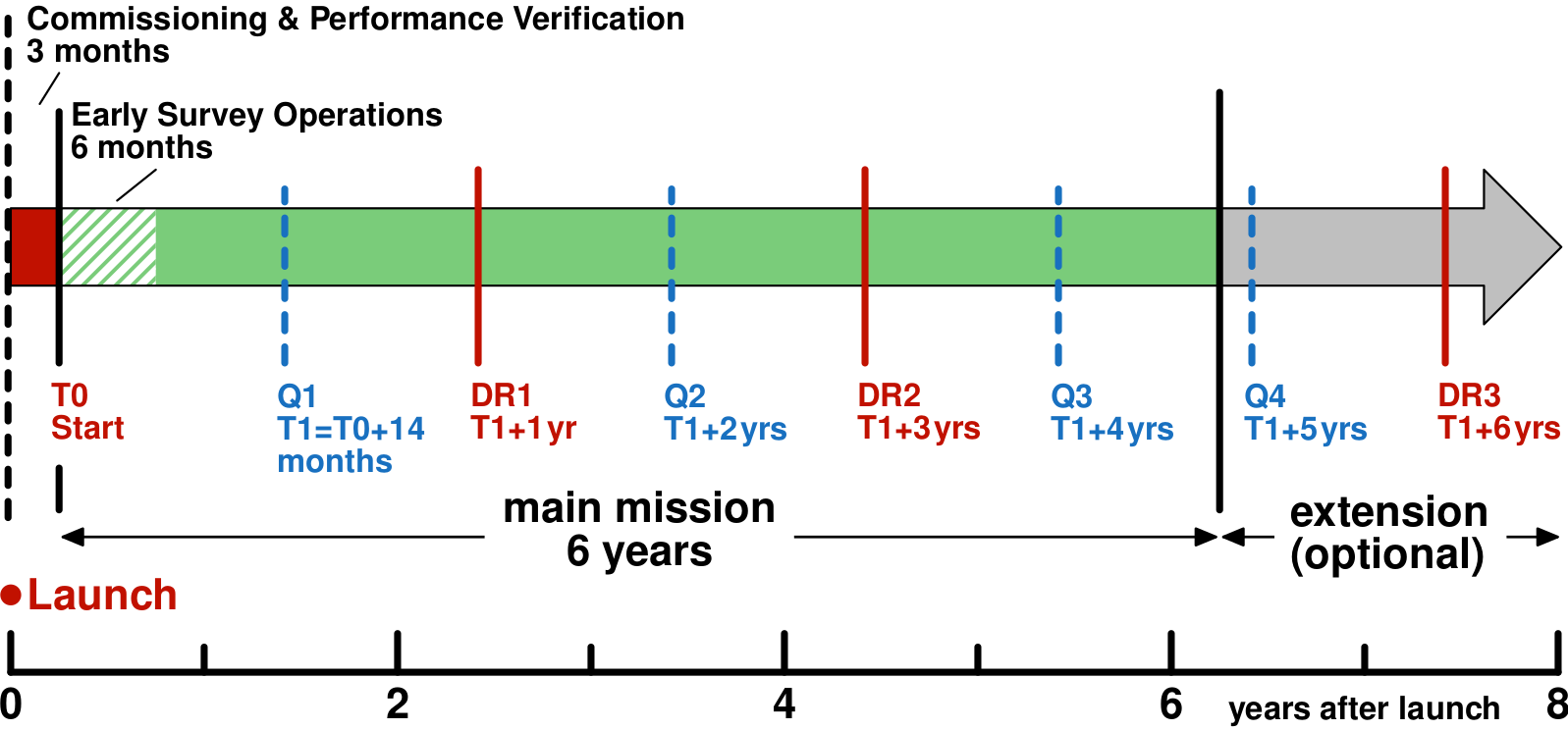
The data processing is also homogenised for each of the three major public DRs. All DRs will occur through the ESA Science Archive, which is already on-line and currently gives access to the Early Release Observations data, presented in accompanying papers. A tentative release schedule, relative to the start of early survey operations, is shown in Fig. 35. The three DRs will contain the complete Euclid data set for roughly the first year of the survey, the first three years of the survey, and the complete survey, respectively. Each DR will comprise all the EWS data products detailed in the preceding sections, similar products obtained on the EDS during the period covered by the DR, as well as the associated calibration products. The SGS software version used for the DR will also be made public at the release time.
As Fig. 35 shows, the DRs are interspersed with so-called quick releases (Q) of smaller volume. At the time of writing, only the contents of Q1 have been planned. This release comprises data for a single visit over the EDFs: 20 deg2 of the EDF-N, 10 deg2 of EDF-F, and 23 deg2 of the EDF-S. We aim to release the imaging and spectroscopic data, as well as catalogues and photometric redshifts.
8 Constraining cosmology with the primary probes
A major development in cosmology since the publication of Laureijs et al. (2011) and the selection of Euclid has been the release of the results from the analysis of Planck data, resulting in cosmological parameter constraints with high precision (Planck Collaboration XVI 2014; Planck Collaboration XIII 2016; Planck Collaboration VI 2020). Moreover, results from other cosmological probes have also continued to improve. As a result, the parameters that describe the concordance CDM model are now well constrained, even though the physical nature of the main ingredients is yet to be explained. Interestingly, in recent years, some inconsistencies between probes have been claimed. For instance, local measurements of the Hubble constant (Riess et al. 2021) differ from the preferred value reported by Planck Collaboration VI (2020). Similarly, weak lensing studies find a lower amplitude for the lumpiness of matter, quantified by (e.g. Asgari et al. 2021). Whatever the origin of these differences, it is clear that the much smaller statistical uncertainties and reduced systematic effects of the Euclid results will have a significant impact in resolving the current debate and defining a new standard model of cosmology.
To exploit the impressive statistical power of Euclid, it is essential that all sources of systematic errors, whether of instrumental, astrophysical, or theoretical origin, are properly identified and their impact fully assessed. This includes assessing the choice of observables, but also the determination of the likelihood and exploring options for the modelling of various systematic effects. Doing so requires a comprehensive analysis of the performance of the mission, from the pixel-level data to the cosmological inference.
In Sect. 8.1 we present the general methodology that has been adopted to assess the impact of systematic errors and describe some of the tools that have been developed to ensure that cosmological constraints derived from Euclid are robust. These efforts are supported by extensive sanity and consistency checks of the data, which in turn drive some of the calibration needs. In Sect. 8.2 we summarise the work done to date to ensure robust parameter estimation, and provide updated predictions for the primary probes. In Sect. 8.3 we explore the prospects of constraining models beyond standard CDM using Euclid.
8.1 Science performance verification
As discussed in Sect. 2, the science objectives that drove the design of the project are to derive precise constraints on the parameters and , which allow us to probe the dynamical nature of dark energy, and to derive constraints on the growth-related parameter. The performance of Euclid for the former is quantified by the FoM defined by Eq. 2. The choices for observables and requirements on residual systematic effects all derive from these core objectives.
It is often not clear how experimental design choices are related to changes in the precision and accuracy with which cosmological parameters can be determined. A first attempt was presented in Laureijs et al. (2011) in order to establish the feasibility of the mission. Since then, new insights have led to additional sources of bias that need to be accounted for, while others may now be better understood. Also, as design choices are made, requirements should be updated, as values derived from generic considerations tend to be conservative (for example, see the discussion in Euclid Collaboration: Paykari et al. 2020, for the weak lensing case).
To quantify how the inferred values of cosmological parameters from a set of observables depend on the adopted underlying cosmological model, uncertainties in our understanding of astrophysical sources of bias, or imperfections in the calibration of the instruments, we have developed tools that enable an end-to-end analysis. This allows us to link changes in the mission design to biases in the cosmological parameters of interest, which in turn helps to prioritise their importance, and to derive requirements for specific steps in the analysis pipelines. This is the main objective of the Science Performance Verification (SPV) exercise.
The basis for this SPV are the EFSs, which provide a sample of realistic galaxies in the redshift range of interest, for both the EWS and EDS. As described in Sect. 6.1, there are multiple purposes of such simulations. In the context of SPV, they are first used to define the set of fiducial values of the reference Euclid model, resulting in a common input catalogue for realistic synthetic observations. As discussed in Sect. 6.2, such simulated data are used to validate the performance of the elements of the pipeline in terms of purity, redshift precision, and photometric performance, as well as evaluating residuals in shape measurements. Such SPV studies also allow us to take global systematic effects into account. For instance, the star density and Galactic extinction varies across the survey. Similarly, radiation damage or ice build-up introduce large-scale variations that need to be quantified.
The performance of individual pipeline elements can be used to approximate the full end-to-end by a series of catalogue-level operations. Although this may not capture all co-dependencies, it provides a fast way to produce catalogues for large areas, while capturing the various sources of bias in a realistic fashion. As an example, biases in shape measurement are introduced by instrumental effects on the scale of the galaxy image. Hence, it is not necessary to create simulated images for a full Euclid survey. Instead, determining the biases as a function of relevant properties for a representative sample is sufficient. These dependencies can then be used to propagate biases at the catalogue level. For instance, Euclid Collaboration: Paykari et al. (2020) used this approach to explore the impact of spatially varying PSF and CTI residuals for the Euclid weak lensing measurements.
8.1.1 Reference observables and nuisance parameters
| Parameters | Fiducial value | Prior | |
|---|---|---|---|
| Cosmology | |||
| Dimensionless Hubble constant | |||
| Present-day physical baryon density | |||
| Present-day physical cold dark matter density | |||
| Dark energy equation-of-state parameters | |||
| Slope primordial curvature power spectrum | |||
| Amplitude of the primordial curvature power spectrum | 3.04 | ||
| Growth index | |||
| Baryonic feedback efficiency factor of the HMCode emulator | |||
| Photometric sample | |||
| Amplitude of intrinsic alignments | |||
| Power-law slope of intrinsic alignment redshift evolution | |||
| Coefficients of cubic polynomial for clustering bias | |||
| Coefficients of cubic polynomial for magnification bias | |||
| Per-bin shear multiplicative bias‡ | |||
| Per-bin mean redshift shift | |||
| Spectroscopic sample | |||
| Per-bin linear bias | |||
| Per-bin second-order bias | |||
| Poissonian shot noise for extra-stochastic parameters | |||
| Per-bin counter term for Legendre monopole | Fixed | ||
| Per-bin counter term for Legendre quadrupole | Fixed | ||
| Per-bin counter term for Legendre hexadecapole | Fixed | ||
| Per-bin purity factor (assuming Poisson distributed interlopers) | |||
‡ We assume a constant nuisance parameter for the multiplicative bias in each photometric redshift bin , which corresponds to the parameter appearing in Eq. 17. The other components (i.e. ) are assumed to be negligible.
As a preparation for the scientific exploitation of Euclid, an evaluation of its performance for the core science goals has been carried out that incorporates our current best knowledge of the mission. Here, we focus on the primary probes (described in Sect. 2) and limit the evaluation using the observables defined in harmonic space.
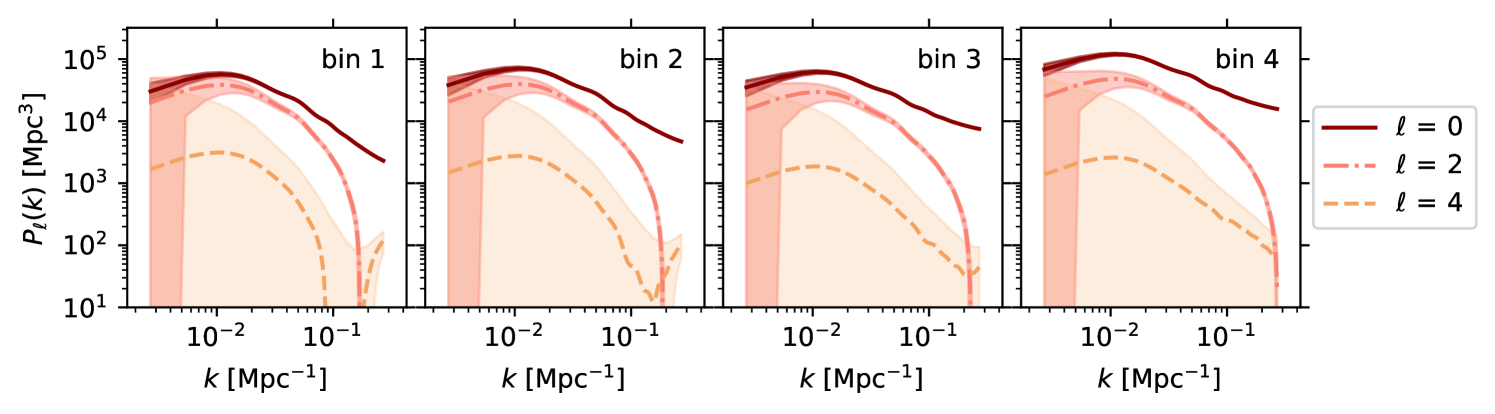
For the spectroscopic clustering measurements, we used the first three even multipoles of the galaxy clustering spectra , defined in Eq. 10. As was done in Euclid Collaboration: Blanchard et al. (2020), we used four redshift bins, with mean redshift values and we used the same binning in . Figure 36 shows the predicted signals for the four redshift bins, where the shaded indicate the uncertainties for the EWS based on the analytical covariance matrix (Sect. 8.1.2). Scale cuts in , which need to be applied for the cosmological inference, were chosen to alleviate so-called projection effects (also known as prior volume effects that shift marginalised posterior distributions; Moretti et al. 2023). We used a maximum value of in the analysis.
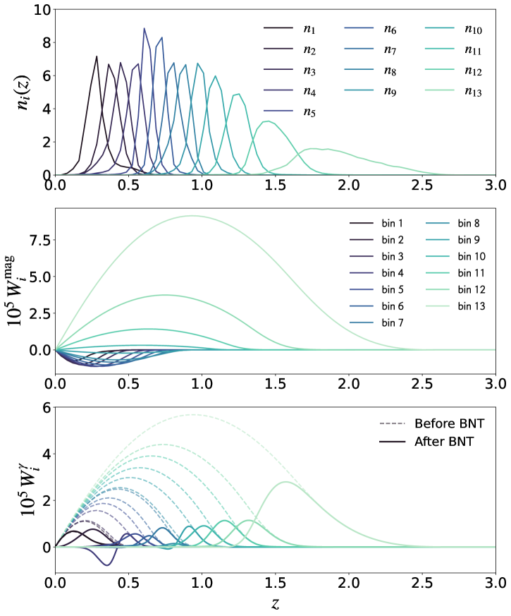
The 3×2pt analysis combines the auto- and cross-angular spectra for the weak-lensing and photometric galaxy-clustering probes. We use 13 equi-populated redshift bins, which are presented in Fig. 37. These are based on photometric redshifts derived from the EFS assuming LSST-like external photometric data (Sect. 7.6.1). As such, these represent the best-case scenario, because the initial analysis will be based on shallower ground-based data. In the following, we also assume that the samples used for weak lensing measurements and photometric clustering are the same. For a more exact treatment, an estimation of the joint errors in photometric redshift and multiplicative bias would be needed.
Although magnification does not improve cosmological constraints, we do need to account for it to avoid biased parameter estimates (e.g. Duncan et al. 2022; Mahony et al. 2022). The middle panel of Fig. 37 shows the magnification kernels, which highlight that magnification is particularly important for the highest redshift bins. The bottom panel shows the shear kernels. We also show results after applying the BNT transformation (Bernardeau et al. 2014; Taylor et al. 2018a), which allows us to control the mixing of scales from LoS projections. Figure 38 shows the synthetic angular power spectra for the weak lensing auto-correlations between the redshift bins, while Fig. 39 shows the corresponding photometric clustering signals. We do not show the cross-correlations, but they are included in the SPV analysis. For the binning in -space we adopted a set of 32 log-spaced bins, ranging from , for the weak lensing and photometric galaxy clustering measurements. This ensures a manageable size of the data vector, but these choices may be adjusted for the actual data analysis. Cuts in are implemented on the observables in harmonic space after BNT transformation, so that accounts for less than 20% of each . For the 3×2pt analysis, we chose for cosmic shear and for angular clustering and galaxy-galaxy lensing.
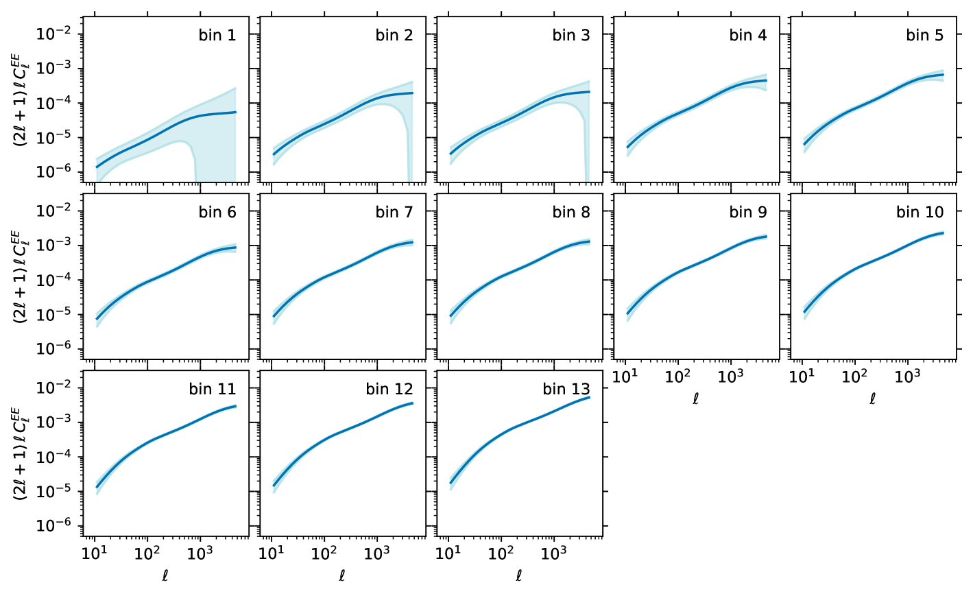
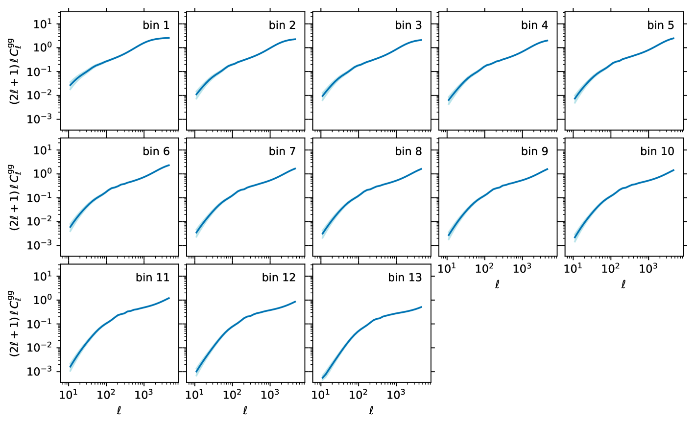
The SPV aims to capture the impact of biases in the data or errors in the modelling itself. In the cosmological inference our ignorance is quantified by nuisance parameters that need to be used consistently, in particular when combining probes. The nuisance parameters can describe astrophysical quantities, such as galaxy biases, or aggregated quantities, such as uncertainties in the purity factor, the mean redshift, or residual multiplicative biases. The nuisance parameters used here are listed and described in Footnote 27. Furthermore, careful modelling needs to take place at nonlinear scales (see Sect. 8.2.2 for details), to ensure that the maximum information encoded at large -values is used to exploit the full Euclid cosmological constraining power. Consequently, a number of key assumptions have been made, regarding the impact of baryonic feedback processes and the modelling of galaxy bias, magnification bias, interlopers, and intrinsic alignments, which all will have to be revisited once data are acquired.
We review the model predictions in Sect. 8.2.2, but briefly discuss our choice for the IA model here. For this study case, we adopt the so-called nonlinear linear alignment (NLA) model (Bridle & King 2007) to describe the scale dependence of the signal, while we assume that the amplitude of the signal scales as
| (25) |
where is the nonlinear growth rate. We assume that the redshift dependence is described by a power law with slope . The amplitude is quantified by the dimensionless parameter , which is scaled by the constant , whose value is determined by the amplitude measured by Brown et al. (2002) in the low-redshift SuperCOSMOS survey (Hambly et al. 2001).
8.1.2 Data covariances
The SPV relies on an accurate estimate of the uncertainties. Hence, attention needs to be paid to the computation of covariance matrices. These are also essential to capture the correlations between probes, redshift bins, and angular scales. For the results presented in Sect. 8.2.1, we made a number of assumptions. First of all, we adopted a Gaussian distribution for the data vector, so that its statistical properties can be entirely characterised by the covariance matrix. Although it might be difficult to go beyond this assumption, we plan to assess its validity in future work. Second, we consider the spectroscopic clustering results to be independent of the 3×2pt measurements. This has been shown to be a reasonable approach for a Euclid-like mission (see Taylor & Markovič 2022). Finally, we evaluated the covariance matrix only for the fiducial model. As shown in Carron (2013), this is required in the Gaussian likelihood approximation to avoid the introduction of spurious parameter information. We assumed that the true model is not too far from the fiducial model (see, e.g. Harnois-Déraps et al. 2019 for a discussion of the impact of this assumption on cosmic shear constraints).
The computation of the covariance matrix of the observables is a challenging task. From a theoretical perspective, the computation of its Gaussian part is well understood. The difficulties arise from the fact that the observed modes are not statistically independent, but are coupled. One dominant source of mode coupling is the nonlinear growth of gravitational instabilities. The effect is particularly important on small scales for the observables in the 3×2pt analysis. The mode coupling through super-sample effects is another significant contributor (see e.g. Euclid Collaboration: Sciotti et al. 2023; Beauchamps et al. 2022). For the SPV analysis this term alone is included since we have found that this should give a realistic estimate. Another source of mode coupling is the impact of masks and visibility functions. When finite volumes and masks have to be taken into account, the harmonic components become coupled (Brown et al. 2005). This depends on the details of the survey, as well as the masking procedures. For now, only the size of the footprint has been taken into account in the SPV exercise – via a rescaling of the covariance by the sky fraction , with the solid angle subtended by the survey, in steradians. A more comprehensive treatment is left for future analysis.
The multi-probe Gaussian covariance is given by (Euclid Collaboration: Blanchard et al. 2020):
| (26) |
In the above equation, the Kronecker delta enforces the aforementioned independence of the different modes in the absence of convolution with the mask. The noise terms are non-zero only for the auto-correlations between probes and tomographic bins:
| (27) |
where is the variance of the total intrinsic ellipticity of the sources. Finally, are the number densities of sources () and lenses (), relevant for cosmic shear and photometric galaxy clustering respectively.
8.2 Expected cosmological parameter constraints
Comparing the Euclid measurements to model predictions is not straightforward, owing to the small statistical uncertainties, the need to marginalise over a large number of nuisance parameters (that are needed to quantify residual systematic effects), our limited knowledge of the nonlinear evolution of structure, and the impact of astrophysical processes on the matter distribution. Moreover, an accurate covariance matrix is needed so that all correlations between measurements can be correctly accounted for. Here, we provide an overview of the tools and procedures that have been developed in order to derive cosmological parameter estimates for Euclid. This updates some previously published forecasts presented in Euclid Collaboration: Blanchard et al. (2020).
8.2.1 CLOE: the Cosmology Likelihood for Observables in Euclid
Given the unprecedented precision of the Euclid data, it is important that the comparison with theoretical predictions uses codes that have been tested rigorously. To this end, we have developed the Cosmology Likelihood for Observables in Euclid (CLOE), a highly flexible modular analysis pipeline written in python3. To ensure the fidelity of the results, the development of CLOE has combined the practices of continuous integration and delivery, enforcing automation in its construction, with careful unit testing and deployment of the code against similar pipelines (Euclid Consortium: Martinelli et al., in prep.).
As a baseline, CLOE provides the theoretical predictions for Euclid’s primary cosmological probes282828The development of CLOE is open to the whole Euclid Consortium, allowing the merging of additional cosmological probes, such as cross-correlations with the CMB or cluster of galaxies. for a given set of cosmological and nuisance parameters. It computes the corresponding likelihood given the measurements (Sect. 7.7) and outputs the posterior probability distributions for the cosmological and nuisance parameters. It relies on the publicly available Boltzmann solvers CAMB (Lewis et al. 2000) and CLASS (Lesgourgues 2011) to compute the theoretical background parameters that are the foundation of the calculations of the primary observables. CLOE computes the predictions for the primary cosmological probes in both harmonic and real space.
A Bayesian approach is used to determine constraints on a given set of cosmological parameters, , given the Euclid data vector, . According to Bayes’ theorem, the key ingredient in the estimation of the posterior distribution of the parameters, , is the likelihood function , which describes the plausibility of a certain parameter value , given a model , after observing a particular outcome. To sample the full posterior distributions of the cosmological parameters of interest, CLOE can be linked to the Bayesian analysis frameworks Cobaya (Torrado & Lewis 2021) and CosmoSIS (Zuntz et al. 2015) as external likelihoods. As a result, CLOE can employ a large number of different MCMC sampling algorithms, such as Metropolis-Hastings, classic nested sampling (e.g. PolyChord; Handley et al. 2015a, b) or advanced nested samplers (e.g. Nautilus; Lange 2023).
Generally, we assume that the likelihood probability distribution of these measurements and the underlying physical model , given the Euclid primary observables , is Gaussian,292929The impact of non-Gaussian terms in the likelihood has been thoroughly studied, and found to depend on the range of scales employed. For our choice of scales for the angular power spectra of photometric probes, non-Gaussian terms have been demonstrated to be negligible for Euclid (Upham et al. 2021; Hall & Taylor 2022). with a covariance matrix that does not depend on cosmology, so that, up to an additive constant,
| (28) |
where is the inverse of the covariance matrix and is the theory vector constructed with the predictions for the Euclid primary observables assuming a cosmological model . CLOE can compute non-Gaussian terms of the likelihood distribution if the type of covariance matrix selected for the statistical analysis is numerical, according to Sellentin & Heavens (2016) and Percival et al. (2022).
Specifically, CLOE consists of a series of semi-autonomous python modules that interface with a Bayesian statistical framework tool, such as Cobaya, to read the relevant data vectors and covariance matrices, to compute the theory vectors (see Figs. 36, 38 and 39), and to calculate the likelihood. The modules that contain the relevant recipes that are needed to compute the theoretical predictions interface with another module that includes the modifications arising from nonlinear structure formation (Sect. 8.2.2). In an exercise of Open Science, CLOE participates in the pilot study case of ESA datalabs303030https://datalabs.esa.int (Navarro et al. 2024) as one the selected Euclid software pipelines to directly interface with the Euclid science archive system in the near future. As a demonstration of the capabilities, all the CLOE-related figures in this paper have been computed using ESA datalabs as the reference analysis framework.
8.2.2 Nonlinear structure formation
A major strength of CMB measurements is that the signal for a given combination of cosmological parameters can be computed directly, because the primary CMB fluctuations are in the linear regime. This is no longer the case for Euclid, unless the cosmological interpretation is restricted to rather large scales. To exploit the information contained in the smaller scales, nonlinear structure formation and the complexities of galaxy formation need to be taken into account. The challenge is to find an appropriate balance between the desire to minimise the statistical uncertainties, whilst ensuring that the predictions are robust. This involves defining the smallest scales that can reliably be used for a particular observable (e.g. Martinelli et al. 2021). The problem is not limited to the signal itself, but also involves robustly quantifying the covariance between measurements at different scales and the combination of observables that probe common structures. As a minimum, this implies a coherent description of the primary probes of Euclid, ensuring that theoretical and astrophysical sources of bias are adequately accounted for. These efforts combine analytical and numerical calculations. Below, we summarise the different approaches that have been adopted to model the various summary statistics from Euclid. We do expect further developments, especially in the implementation of emulators (e.g. Eggemeier et al. 2022; Pellejero-Ibanez et al. 2022). As a first step, efforts have focused on analytical prescriptions and emulators that have been extensively validated with simulations and used in some of the most recent data analyses (e.g. Bose et al. 2020; Arnold et al. 2022; Carrilho et al. 2023; Piga et al. 2023).
For the spectroscopic galaxy clustering probe, we need to model the nonlinear galaxy power spectrum in redshift space. We will use a 1-loop perturbation theory model, with counter-terms computed using the effective field theory (EFT) of LSS (Ivanov et al. 2020; d’Amico et al. 2020), which allows us to predict the clustering of matter in the mildly nonlinear regime. To this end, we have developed a new code (Moretti et al. 2023) using the FAST-PT algorithm for the loop-integral evaluations (McEwen et al. 2016; Fang et al. 2017). The code has been validated against -body simulations (Oddo et al. 2021; Tsedrik et al. 2023, also see Fig. 2) and has been used for the re-analysis of BOSS data (Moretti et al. 2023; Carrilho et al. 2023).
For the analytical covariance, the prescription of Wadekar & Scoccimarro (2020) is used, including contributions from nonlinear effects, the window function, super-survey modes, and the integral constraint. As part of the analysis of BOSS DR12, this prescription has been shown to be in excellent agreement with the covariance estimated from over 2000 numerical mocks up to , leading to negligible differences in cosmological parameters using either approach (Wadekar et al. 2020).
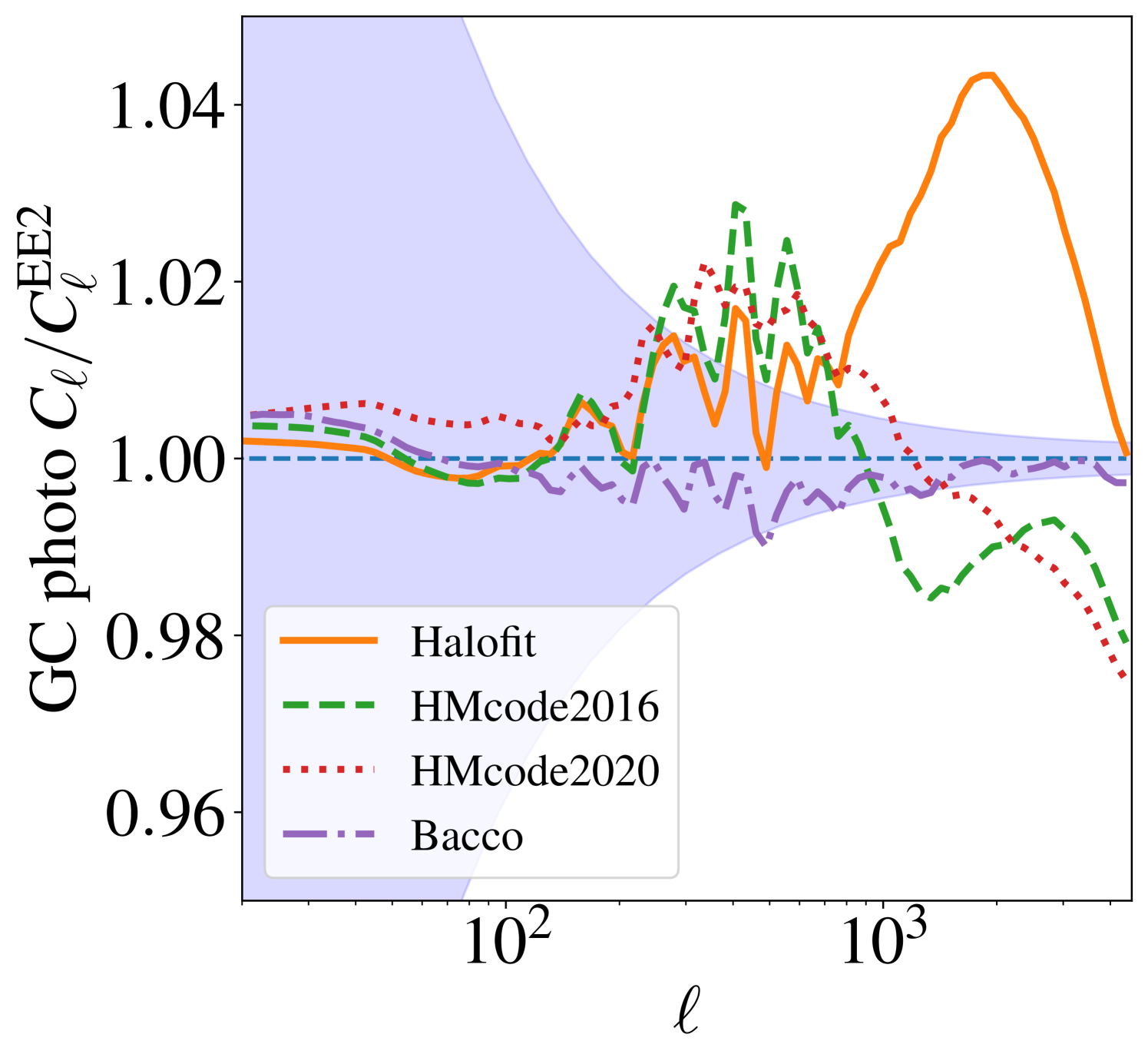
The modelling of the 3×2pt signals presents its own challenges, because of the desire to probe the matter power spectrum on nonlinear scales, and the need to account for baryonic feedback for the shear-shear and galaxy-shear correlations (Semboloni et al. 2011). In this case, two emulators, based on -body simulations, have been developed and validated. The resulting Euclid Emulator (Euclid Collaboration: Knabenhans et al. 2019) and the bacco emulator (Angulo et al. 2021) can predict the nonlinear power spectrum with an accuracy of about out to in the redshift range , and include predictions for massive neutrinos and CDM. Ongoing development of these emulators aims to ensure that their accuracy is sufficient for the analysis of the Euclid data. For baryonic feedback effects, we have implemented the BCEmu (Giri & Schneider 2021) and bacco (Aricò et al. 2021) emulators. Other popular prescriptions like halofit (Smith et al. 2003; Takahashi et al. 2012) and HMCode (Mead et al. 2016, 2021) are also available (see Fig. 40). Ongoing simulated data challenges will determine the minimum number of baryonic feedback parameters needed for unbiased parameter inference and the associated scale cuts required, while we also plan to implement nonlinear and non-local bias models for photometric galaxy clustering with prescriptions based on either perturbation theory (Pandey et al. 2020) or hybrid emulators for biased tracers (Zennaro et al. 2023).
As alluded to in Sect. 2.2, we need to account for intrinsic alignments of galaxies (Joachimi et al. 2015; Troxel & Ishak 2015). To capture a wide range of possible alignments, we have implemented the tidal alignment and tidal torque (TATT) model (Blazek et al. 2019), used in the DES cosmic shear analyses (see e.g. Troxel et al. 2018). Progress will come from linking IA models to observations, including those made by Euclid, so that the dependence of the IA signal on galaxy properties can be used to reduce the number of nuisance parameters (Fortuna et al. 2021).
Finally, to consistently model the correlations between scales, tomographic bins, and the different probes, we need an accurate covariance matrix for the 3×2pt measurements. Currently, several independent codes have been studied and validated, including the PySSC module (Lacasa & Grain 2019). Thus far, the focus has been on quantifying the impact of super-sample covariance, which is the largest of the expected non-Gaussian contributions (Barreira et al. 2018; Upham et al. 2022; Beauchamps et al. 2022; Euclid Collaboration: Sciotti et al. 2023).
We also want to explore models that include complexity beyond the baseline CDM model (see Sect. 8.3). Although the range of possibilities is vast, we have focused the development on the main science objectives of Euclid. Hence, we have included nonlinear modelling prescriptions for CDM, , and massive-neutrino cosmologies. Ongoing efforts include developing and implementing nonlinear models for a suite of exotic dark energy and modified gravity cases.
8.2.3 Parameter estimation
Since the estimates for the performance of Euclid were presented in Laureijs et al. (2011), the fidelity of the predictions has steadily improved. In particular, Euclid Collaboration: Blanchard et al. (2020) presented results from the first collaborative analysis to verify forecasting tools. This study focused on forecasts based on Fisher matrix techniques applied to both primary probes. A key aspect involved the comparison of different numerical implementations. The results showed optimistic and pessimistic scenarios for several cosmological models (flat and non-flat, and different cuts of the nonlinear scales), highlighting the role of the cross-correlations, especially for models beyond a cosmological constant, potentially increasing the dark energy FoM by at least threefold.
In this section, we update the forecasts from Euclid Collaboration: Blanchard et al. (2020) using the primary probes only (see Sect. 8.1.1 for details about our setup). We limit the discussion to the baseline models of interest: a spatially flat cosmological model, using Eq. 1 to describe the dark energy equation of state (CDM); and a model where the parameter is left free (CDM + ).
We generated synthetic noiseless data vectors by running CLOE v2.0.2 (Euclid Consortium: Joudaki et al., in prep.) using the fiducial values for the cosmological model parameters presented in Footnote 27. For this analysis we used the analytical super-sample covariance matrix for the 3×2pt observable (see Euclid Collaboration: Sciotti et al. 2023), and a Gaussian covariance matrix for the spectroscopic probe (GCsp), following the specifications of the SPV exercise for the survey area and other experimental systematics. For the correction of the matter power spectrum at nonlinear scales, we used the latest version of HMcode (Mead et al. 2021) for the photometric probes (allowing the baryonic feedback efficiency factor of the code emulator, , to be free) and a 1-loop perturbation theory model based on FAST-PT for the spectroscopic measurements, as described in Sect. 8.2.2.
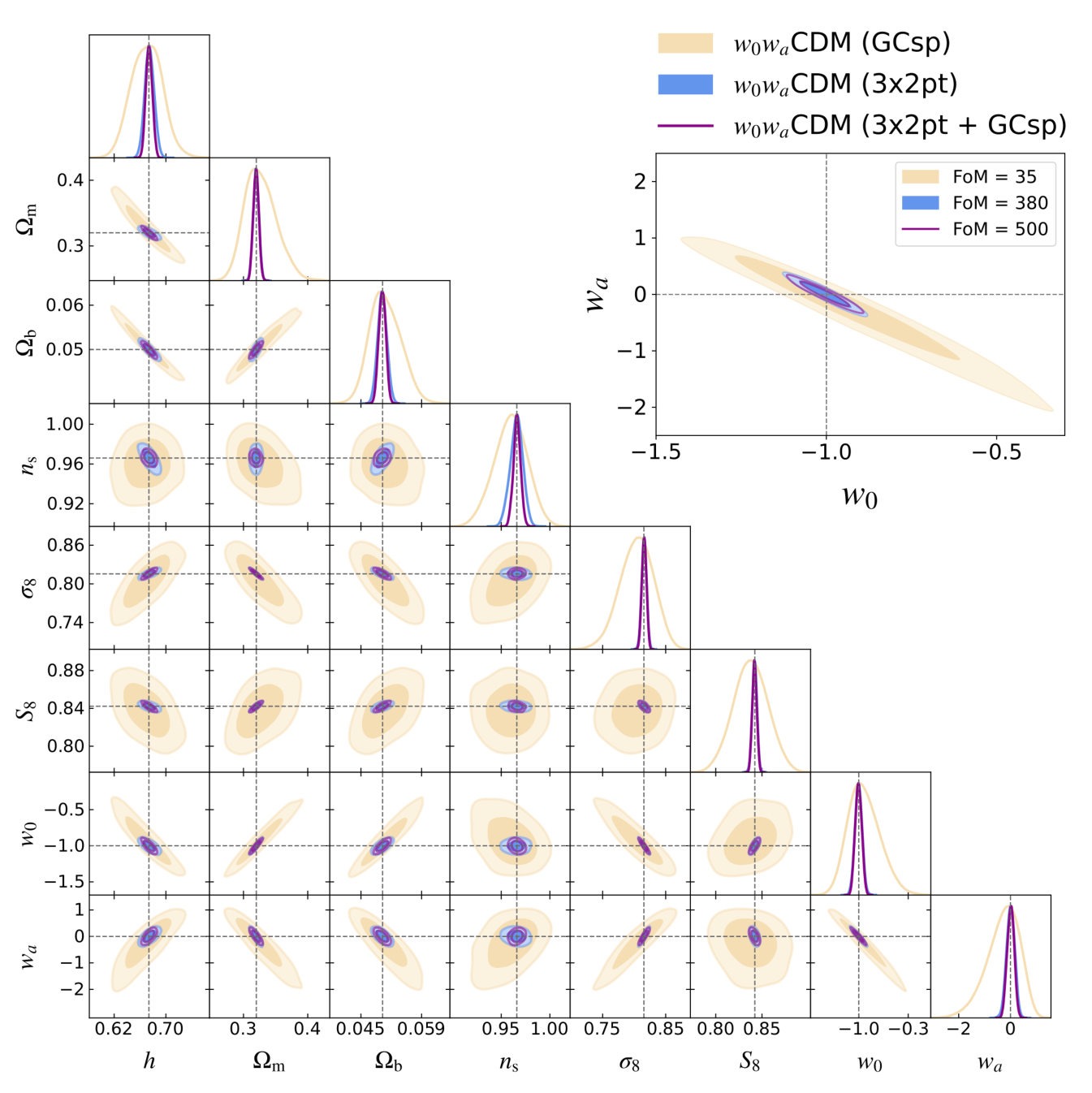
The corresponding theoretical predictions and the calculation of the Euclid likelihood (see Eq. 28) were computed using CLOE v2.0.2. The sampling of the posterior distributions were obtained using the novel nested sampler Nautilus, interfaced with Cobaya, imposing the priors for all the free cosmological and nuisance parameters presented in Footnote 27. For forecasting purposes, and to speed up the sampling process, we have used BBN information as a Gaussian prior for the baryon density parameter (Cooke et al. 2018). In this section, we show the results corresponding to three different forecasting cases: 3×2pt, GCsp and 3×2pt + GCsp (see Euclid Consortium: Cañas-Herrera et al., in prep, for a more complete discussion of the forecasts with CLOE). For the GCsp case, we need to sample a total of 23 free parameters, while we need 44 free parameters for the 3×2pt case, and 60 for the joint one. Moreover, we track several derived parameters on the fly, and simultaneously fit 364 (3×2pt) and 12 (GCsp) different spectra. During the analysis, we have fixed the per-bin counter terms (see Footnote 27) in the 1-loop perturbation theory model used for the GCsp probe, in an effort to mitigate the so-called projection effects. We thus implicitly assume that in future analyses we will be able to impose tighter priors on these model nuisance parameters. To achieve convergence, the parameter space is explored by calculating the Bayesian evidence using 4000 live points313131In nested sampling, a live point is a sample of the likelihood distribution as given by the prior, that is later used to construct the evidence. in each iteration. To obtain the results presented here, we used approximately 0.2 million CPU hours in total.
Figure 41 shows constraints on the dark energy parameters and , as well as the corresponding constraints on the other cosmological parameters, while Fig. 42 shows constraints on the parameter. Regardless of the cosmological models, similar converged distributions are obtained for the nuisance parameters. For all the cases, the fiducial values are recovered for all the sampled parameters, with associated uncertainties that improve by one order of magnitude compared to current surveys (Abbott et al. 2022). The values obtain for the FoM of the dark energy parameters and are consistent with those of Euclid Collaboration: Blanchard et al. (2020), and they are obtained by marginalising over all the sampled parameters.
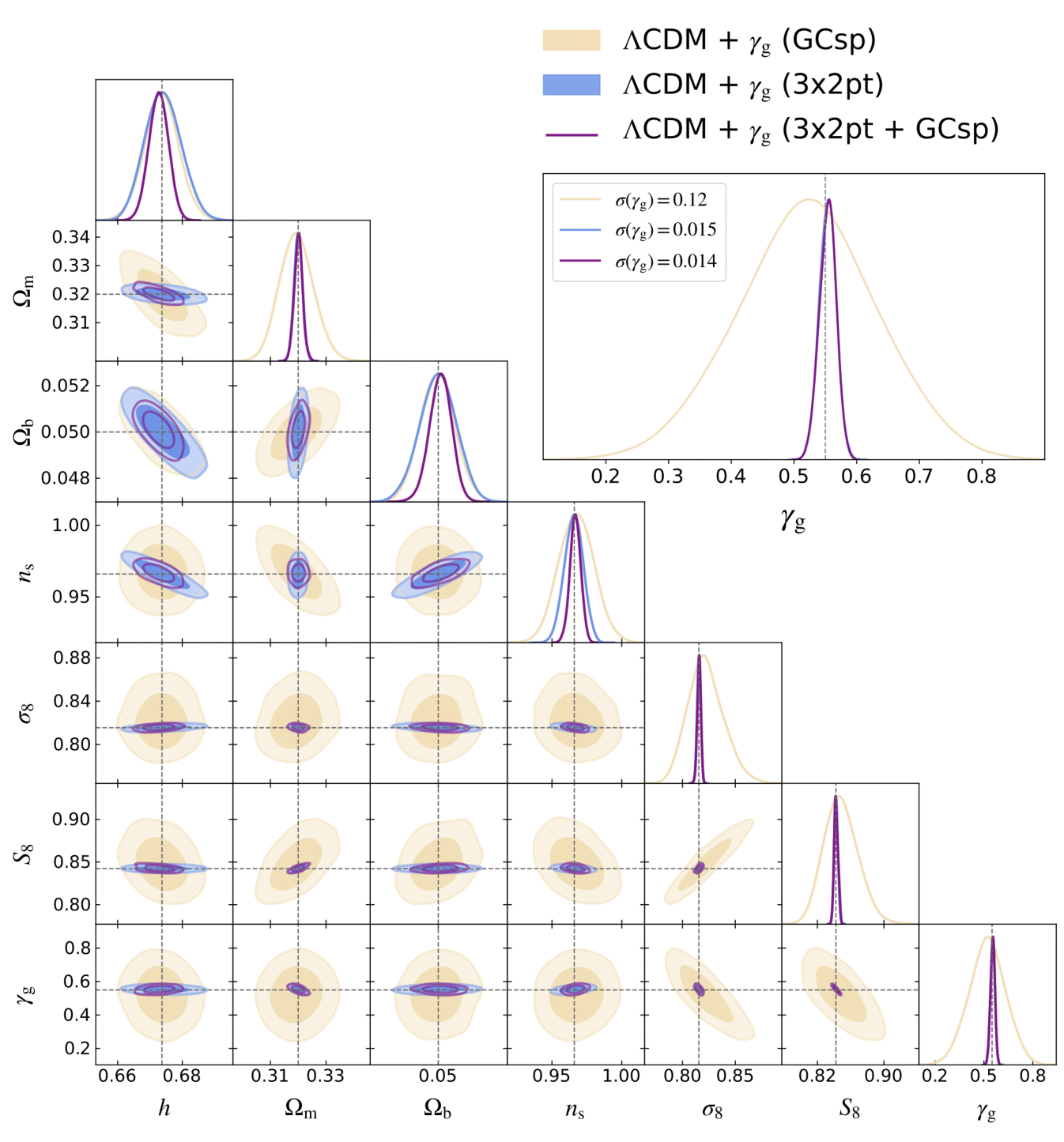
8.2.4 Blinding strategy
Cognitive bias of the scientists undertaking an experiment can lead to priors on data analyses linking together otherwise independent measurements. Blinding strategies are designed to broaden these priors by separating the influence of the scientists’ predictions for the measurements from the results themselves. We aim to avoid such biases introduced by the way data are processed, selected, or modelled. This requires some care, because the tendency to either consciously or unconsciously select, process, or interpret data in such a way as to confirm prior beliefs often leads to biased results (Nickerson 1998). The quest to determine cosmological parameters is no exception (Croft & Dailey 2011) because certain values for cosmological parameters may be preferred based on theoretical grounds.
Many recent cosmological analyses have taken steps to avoid cognitive bias by adopting a so-called ‘blinding’ strategy. This can take many forms, for example, by shifting values or theoretical models in plots (e.g. Wong et al. 2020), modifying the data vectors (e.g. Muir et al. 2020), or adjusting the covariance matrix (Sellentin 2020). The Euclid data are required to pass stringent validation tests, while the software that is employed to process the data is under strict control. This distinguishes it from most previous cosmological experiments, but there is still the potential to introduce biases during the scientific analysis.
The blinding strategy we propose for Euclid starts with the extensive use of synthetic data, such as those described in Sect. 6.2, to build and test pipeline elements. We will then allow the analysis of the first 500 deg2 observed at the start of the project without any blinding. This represents of the expected final sample. Assuming that variance scales with the inverse of the volume, the results from the early data should have an error 5.5 times larger than that from the final data and should be comparable to current constraints. Thus we can consider that analysing this sample is equivalent to blinding the signal at the 5.5 level. As the pipeline is developed and refined before the first data release (DR1; Sect. 7.8), development will concentrate on this sample, and it will be the only sample upon which revisions in the pipeline are retrospectively applied until the DR1 sample is constructed.
As described in Sect. 4.3, the Euclid mission has defined a careful and comprehensive calibration strategy. The observations taken to facilitate the calibration tend to use the instrument in a different way to the EWS, so that potential systematic problems can be identified and quantified. Crucially, the calibration measurements do not strongly depend on cosmology, and hence can be analysed without additional blinding.
For the core cosmology measurements to come from DR1, we adopt a strategy similar to that adopted by the DES (Muir et al. 2020), but without forcing the shift to match between galaxy clustering and weak lensing measurements. Independent shifts mean that differences between statistics are blind: while we cannot then use them to test our analysis methodology, the impact of Euclid on any tensions will be blinded. We choose to introduce blinding at the level of derived statistics rather than raw data to facilitate calibration and validation tests and to ensure we do not impact other analyses of these data.
Specifically, we will shift the two-point data products (e.g. the correlation function and power spectrum multipole moments) by the expected difference between two cosmological models. This includes shifts in the effects of all of the key cosmological processes to be measured. The model offset applied will be between the best-fit flat CDM model of Planck Collaboration VI (2020), and one randomly chosen within a 3 interval.
8.3 Beyond CDM models
As shown above, the primary probes of Euclid will place tight constraints on the parameters of the CDM model. However, as already highlighted in Sect. 2, the data also greatly advance our ability to explore various extensions to the standard cosmological model, potentially shedding light on the dark constituents of the Universe and the underlying theory of gravity. Here, we highlight some of these cases, where we note that further improvements can be achieved when combining the Euclid results with complementary cosmological probes, such as the ones summarised in Sect. 9.
The combination of the primary probes over the EWS area offers the unique opportunity to test gravitational physics on cosmological scales, placing constraints on several modifications of GR and models of dark energy (Amendola et al. 2018). In addition to testing specific models, more agnostic descriptions of modified gravity and dark energy can be explored. For instance, the phenomenological functions and parameterise, respectively, the relation between the matter density contrast and the Newtonian and lensing potentials in Fourier space (e.g. Pogosian et al. 2010), while the EFT of dark energy (Frusciante & Perenon 2020) provides a framework to explore deviations from GR consistently. Provided the observables can be modelled accurately on nonlinear scales, Euclid will provide outstanding constraints on extensions of CDM, especially when cross-correlations with CMB measurements are also included (see Sect. 9.4; Casas et al. 2023; Frusciante et al. 2023).
Massive neutrinos suppress the matter power spectrum on small scales. Hence, a measurement of this subtle signature allows the sum of neutrino masses, , to be constrained using cosmological data. Current CMB and LSS measurements provide stringent upper bounds (, 95% confidence; Planck Collaboration VI 2020; Alam et al. 2021; Palanque-Delabrouille et al. 2020), well below the limits of current laboratory experiments studying decay (upper limit on effective electron anti-neutrino mass , 90% confidence, Aker et al. 2022). The absolute neutrino mass sum is still unknown, but this situation will change thanks to Euclid. In the minimal CDM+ model, Euclid’s primary probes alone can constrain the neutrino mass with a error for a fiducial neutrino mass of . In combination with Planck, a precision of can be reached, implying a detection of a non-zero neutrino mass (Euclid Collaboration: Archidiacono et al. 2024). If the true neutrino mass is below , these constraints will also provide evidence in favour of the normal neutrino mass ordering.323232The minimum mass allowed by neutrino oscillation experiments in normal (inverted) ordering is (). We note that these estimates are conservative because they assumed the pessimistic scenario of Euclid Collaboration: Blanchard et al. (2020). Ongoing efforts to improve the modelling of nonlinear structure formation (Sect. 8.2.2) should ultimately result in smaller uncertainties.
Euclid will also improve the constraints on the effective number of relativistic degrees of freedom , which accounts both for the number of standard model neutrinos (, Froustey et al. 2020; Bennett et al. 2021) and for additional light particles, dubbed ‘dark radiation’. The sensitivity of Euclid, in combination with current and future CMB surveys, to will potentially exclude several theoretically well-motivated particles beyond the standard model (Euclid Collaboration: Archidiacono et al. 2024). Therefore, Euclid will also shed light on dark matter models predicting a deviation of from the standard model value, such as models involving interactions between dark matter and dark radiation. Moreover, Euclid will inform the models for alternative dark matter scenarios beyond the cold dark matter paradigm, by improving the constraints on warm dark matter, and decaying dark matter (Euclid Collaboration: Lesgourges et al., in prep.).
Current observations are consistent with initial conditions that correspond to a flat Universe with nearly Gaussian adiabatic perturbations, whose spectrum is described by a simple power law (Planck Collaboration I 2020; Alam et al. 2021). Thanks to the different sensitivity of the primary probes to the expansion of the Universe and to the growth of structure, Euclid provides an invaluable snapshot of the initial conditions at low redshift. The measurements will reduce the uncertainty on the spatial curvature an order of magnitude below the current constraints from galaxy surveys (Alam et al. 2021). A similar improvement is expected for the uncertainty in the value of the scalar spectral index and its running . Euclid will also improve the constraints on features in the primordial power spectrum as forecast in Ballardini et al. (2024).
Euclid will test the statistics of primordial fluctuations beyond the power spectrum. The spectroscopic survey is expected to improve constraints on , the local shape of primordial non-Gaussianity, by approximately a factor 8 over current results (Mueller et al. 2022), reaching an uncertainty of about when combining power spectrum and bispectrum information and assuming universality for the halo mass function. These uncertainties on initial conditions are comparable to those obtained by Planck (Planck Collaboration X 2020; Planck Collaboration IX 2020), but target a markedly different range in redshift and scale.
9 Additional cosmological probes
Euclid is designed with the primary probes in mind, but the data enable a wide range of additional measurements that can improve cosmological parameter constraints (Laureijs et al. 2011). For instance, the cosmological information is not limited to the two-point statistics that we have focused on so far. In Sect. 9.1 we discuss how higher-order clustering and lensing statistics can be used to improve cosmological parameter constraints. In Sect. 7.7.4 we already highlighted the large number of clusters that Euclid will discover. Their use to improve cosmological parameter constraints is reviewed in Sect. 9.2. As discussed in Sect. 9.3, the sharp imaging data are ideal for the discovery of strong gravitational lenses, which enable a unique study of the distribution of dark matter on small scales, as well as additional tests of cosmology. The wide area galaxy and matter maps (see Sect. 7.7.3) can be cross-correlated with measurements of the CMB, enabling new probes that are presented in Sect. 9.4. Finally, high-redshift quasars with X-ray data can complement low-redshift cosmological probes in the determination of the cosmological parameters as discussed in Sect. 9.5, while Sect. 9.6 explores the use of passive galaxies as chronometers to provide an independent constraint on the expansion history.
9.1 Higher-order statistics
While the two-point statistics would capture all cosmological information in the LSS if it were Gaussian, nonlinear structure formation has introduced non-Gaussian features into the cosmic matter distribution. The full information content can, therefore, only be unlocked with higher-order statistics (HOS). A wide variety of observables that capture the higher-order information have been proposed, which can be roughly grouped into two categories: those that consider -point correlation functions and th-order moments of the density distribution; and those that use topological information of the density distribution. Examples for the first category are higher-order moments (e.g. Gatti et al. 2022; Porth & Smith 2021), higher-order correlation functions (e.g. Heydenreich et al. 2023; Burger et al. 2024) and one-point probability distributions (e.g. Barthelemy et al. 2020; Boyle et al. 2021). The second category includes peak statistics (e.g. Martinet et al. 2018; Harnois-Déraps et al. 2021), Minkowski functionals and persistent homology (e.g. Parroni et al. 2020; Heydenreich et al. 2022), and scattering transforms (e.g. Cheng et al. 2020; Cheng & Ménard 2021). Many estimates can be inferred from WL convergence maps (see Sect. 7.7.3), while some, for example, higher-order correlation functions and aperture mass moments, can be directly measured from shear catalogues (Jarvis et al. 2004; Secco et al. 2022; Porth et al. 2023).
When combined with two-point statistics, HOS enhance cosmological constraints by (partially) resolving parameter degeneracies (e.g. Kayo & Takada 2013; Heydenreich et al. 2023). Euclid Collaboration: Ajani et al. (2023) found that combining each of ten different WL HOS with two-point statistics results in a twofold improvement in constraining and compared to relying solely on two-point statistics. Combining all HOS leads to a factor of about 4.5 improvement.
The power of HOS is illustrated in Fig. 43, which shows expected constraints from a Fisher forecast analysis on and with all other cosmological parameters fixed, using the shear correlation functions , the convergence PDF, or the combination of both. The covariance for the analysis is estimated from the Scinet LIghtCone Simulations (SLICS) -body simulations (Harnois-Déraps et al. 2018) and the derivatives of the data vectors are taken either from theoretical predictions (see Boyle et al. 2021 for details on the PDF modelling) or from the DUSTGRAIN-pathfinder simulations (Giocoli et al. 2018), where for the simulations we used the Kaiser–Squires mass reconstruction scheme (see Sect. 7.7.3) The PDF shows a different degeneracy direction between and than the second-order statistics, illustrated by the tilted ellipse in the lower-left corner of Fig. 43. This change in the degeneracy leads to a tightening of the constraints on and when and the PDF are combined. Consequently, the HOS carry additional cosmological information, which needs to be included to unlock all of Euclid’s potential.
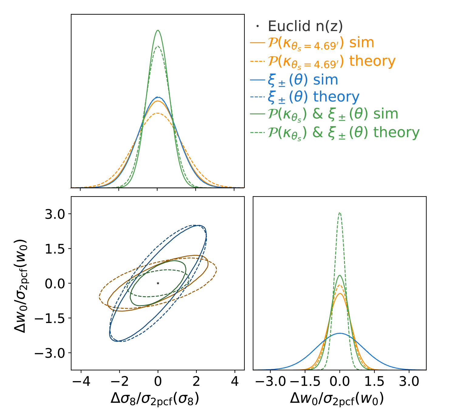
HOS can also test for residual systematics and constrain astrophysical effects such as intrinsic alignment (Pyne & Joachimi 2021), baryonic feedback (Semboloni et al. 2013b), or galaxy bias (Huterer et al. 2006). Since the HOS react differently to these effects than two-point statistics, combined analyses allow us to simultaneously constrain cosmological and nuisance parameters without additional data sets.
9.2 Clusters of galaxies
Galaxy clusters have long proven to be a valuable cosmological tool (e.g. Bahcall & Fan 1998; Borgani et al. 2001; Haiman et al. 2001; Weller et al. 2002; Reiprich & Böhringer 2002; Vikhlinin et al. 2009; Mantz et al. 2015; Planck Collaboration XXIV 2016; Bocquet et al. 2019; Costanzi et al. 2019; DES Collaboration et al. 2020; Lesci et al. 2022; Chiu et al. 2023; Ghirardini et al. 2024). Arising from the highest density peaks of the initial matter density field, the abundance and spatial distribution of clusters contains information on the growth of structures and expansion history of the Universe (Allen et al. 2011; Kravtsov & Borgani 2012). More specifically, the cluster abundance is a sensitive probe of the parameter . The evolution of cluster counts, which effectively measures the growth rate of cosmic structure, constrains dark energy and modified gravity models (e.g. Mantz et al. 2015; Cataneo et al. 2015; Bocquet et al. 2019). The galaxy cluster correlation function, probing the same matter field traced by galaxies, is sensitive to the same cosmological effects and parameters detailed in Sect. 2.1. The relative lower S/N of the cluster clustering measurement, due to the sparser nature of the cluster sample, is mostly compensated by a theoretically predictable halo bias (e.g. Sartoris et al. 2012). The combination of cluster counts and clustering has the potential to deliver independent, competitive, and complementary cosmological constraints to those provided by the primary Euclid probes, but depends sensitively on our ability to accurately calibrate their masses (Sartoris et al. 2016; Fumagalli et al. 2024). Indeed, while it is possible to predict with percent level accuracy the abundance of dark matter halos as a function of mass and redshift in an arbitrary cosmology (e.g. Tinker et al. 2008; Castro et al. 2021), halo masses themselves are not directly observable. In cluster cosmology studies, it is hence crucial to identify and calibrate observational proxies – such as the number of member galaxies (richness), X-ray luminosity, or the Sunyaev–Zeldovich (SZ) signal – against mass. At present, the calibration of these scaling relations represents the main limiting factor for cluster cosmology studies at all wavelengths (e.g Planck Collaboration XXIV 2016; DES Collaboration et al. 2020).
The combination of Euclids wide sky coverage and high-quality optical data will allow the detection of an order of clusters above out to redshift 2, increasing the number of detected systems by more than an order of magnitude compared to current surveys (Sartoris et al. 2016). In particular, Euclid will perform a census of the cluster population above for the first time in the optical-NIR wavelength regime, a critical stage of the Universe’s evolution for studying dark energy. The unprecedented large statistics, along with the large volume probed by the survey, will allow Euclid to beat down shot noise and sample variance, enabling a statistically significant measurement of the cluster correlation function at . Along with the exquisite imaging data provided by Euclid s space observations, this will enable a weak lensing calibration of the observable-mass relation out to (Köhlinger et al. 2015), while the sparse spectroscopic data for cluster-member galaxies at will provide a valuable mass proxy for high-redshift systems (Sartoris et al. 2016).
The large number of clusters and the precision of the lensing measurements demand stricter control over systematic effects compared to current cluster surveys. This is especially true for a photometric cluster survey such as Euclid’s, capable of detecting systems down to group mass scales and becoming mass-complete above (see Sect. 7.7.4). These systems, which outnumber their more massive descendants by orders of magnitude, potentially encode valuable cosmological information, but prove to be difficult to include in abundance studies (DES Collaboration et al. 2020); the limited resolution that a photometric cluster-finder algorithm can achieve along the LoS leads to unavoidable uncertainties and biases in the richness estimate, which become more severe in the low-S/N regime. The correlation of these systematics with others affecting the lensing measurements, or dynamical mass proxies, further hampers the characterisation of these systems (Sunayama et al. 2020; Wu et al. 2022). For Euclid, the calibration of such selection effects, as well as the determination of the threshold for the minimum cluster richness, will be tackled using a combination of simulated and multi-wavelength data analyses (e.g. Costanzi et al. 2019, 2021; Grandis et al. 2021), along with the inclusion of the clustering of clusters statistics. The latter, thanks to the mass dependence of the halo bias, will enable us to break the degeneracy between cosmological and scaling-relation parameters when combined with the other cluster observables (e.g. To et al. 2021). In summary, from the combination of cluster counts, cluster clustering, and Euclid s mass-proxies, we expect to increase the precision on the estimation of by an order of magnitude compared to current galaxy cluster studies based on imaging surveys, such as DES and KiDS, or SZ surveys, such as Atacama Cosmology Telescope (ACT) and South Pole Telescope (SPT). Moreover, Euclid’s ability to sample the cluster population at will ensure an improvement of a factor of 2 on the DE FoM, compared to cluster surveys at lower redshift (e.g. Sartoris et al. 2016; Bocquet et al. 2019).
Furthermore, the inclusion of Euclid weak lensing data is expected to dramatically improve the cosmological constraints derived from intra-cluster-medium-selected cluster samples, such as the ones provided by the extended ROentgen Survey with and Imaging Telescope Array (eROSITA; Bulbul et al. 2024), or the high-resolution SZ surveys conducted by SPT (e.g. Bleem et al. 2015; Benson et al. 2014) and ACT (Hilton et al. 2021).
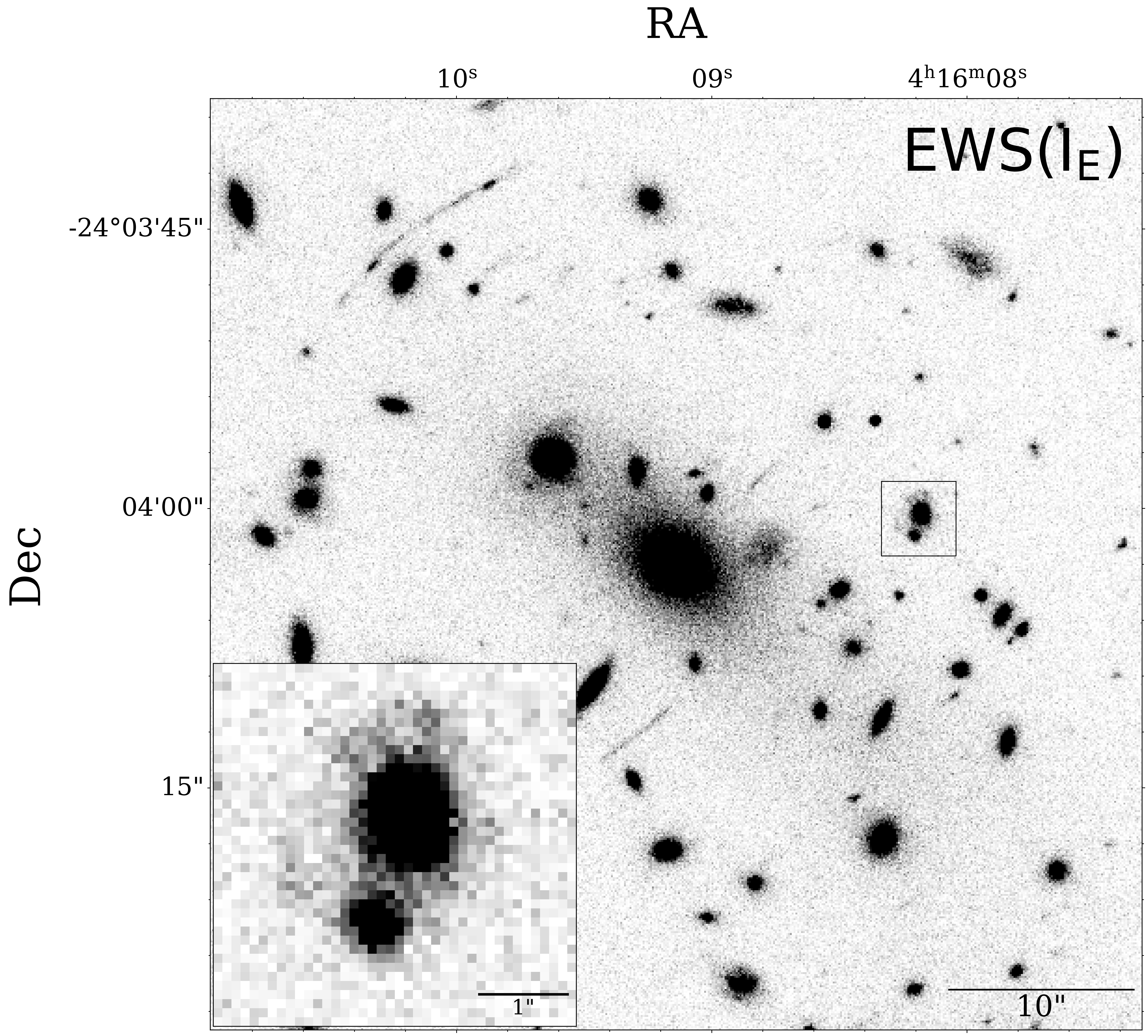
9.3 Strong gravitational lensing
Multiple images of a distant source can be produced if light rays pass sufficiently close to a massive structure along the LoS. Such favourable configurations are rare, and typically are not resolved in ground-based observations. Thanks to the sharp images provided by Euclid, vast numbers of strong lenses will be discovered, and we highlight some of the main applications here. Strong lensing studies with Euclid will cover a wide range of mass, from galaxies to groups and clusters of galaxies (see e.g. Fig. 44), while probing the distribution of dark matter on relatively small scales.
We expect to detect approximately 200 000 galaxy-scale strong lenses, which thus make up the largest fraction of systems. These typically feature an lens at a median redshift within the EWS. The sources in these systems are expected to have redshifts ranging from (Collett 2015; Metcalf et al. 2019; Euclid Collaboration: Leuzzi et al. 2024), resulting in an average Einstein radius of , which aligns well with the capabilities of Euclid, but is too small for ground-based surveys (e.g. Petrillo et al. 2019). In the EDS, approximately 3500 lenses are expected, compared to 500 in the equivalent area of the EWS. On average, the unlensed magnitude of the sources is 2 magnitudes fainter than that of the lensed ones, highlighting the significant magnifying effect of lensing (Lotz et al. 2017). This magnification enables the search for ultra-high redshift (lensed) sources up to in the EDS, down to an unlensed magnitude of 28. This approach is critical for investigating questions about re-ionisation by distant protogalaxies. As Euclid targets the Ly line and benefits from magnifications up to (Mason et al. 2015; Atek et al. 2015; Vanzella et al. 2017a), we anticipate the discovery of 35 to 75 such galaxies in the EDS, while brighter and rarer events may be discovered in the EWS. Moreover, in spite of the lower NISP resolution, in the EWS we expect to find tens of thousands of bright lensed NIR sources in the NISP photometric data that are too faint to be detected in the band (Pearson et al. 2024). Most of these will be sub-millimetre galaxies (at –4) or evolved red galaxies.
We expect the identification of up to 2300 lensed quasars, with approximately 16% predicted to be quadruply imaged (Oguri & Marshall 2010). The discovery of lensed supernovae (e.g. Pascale et al. 2024) will complement the lensing of quasars; due to the EDS observations being divided into roughly 40 independent epochs over the six-year mission duration, the detection of several lensed type-Ia supernovae is expected. Both lensed quasars and supernovae will facilitate time-delay cosmography (Treu et al. 2022), allowing for measurements of the Hubble constant (Refsdal 1964; Kelly et al. 2015; Grillo et al. 2018; Wong et al. 2020). This process requires adding the time dimension to the precise Euclid data, demonstrating a significant synergy with LSST.
Moreover, microlensing in lensed quasars can be utilised to estimate the fraction of dark matter in compact form in galaxies (Mao & Schneider 1998; Moustakas & Metcalf 2003; Koopmans 2005; Vegetti & Koopmans 2009; Vegetti et al. 2012; Hezaveh et al. 2016; Nierenberg et al. 2017; Gilman et al. 2020; Wagner-Carena et al. 2023; Powell et al. 2023). Analysing the flux ratios between lensed images or their distribution across the sample of lensed quasars provides insights into the quantity and distribution of low-mass dark matter halos in lensing galaxies and along the line of sight (LoS). High spatial resolution follow-up observations, using very-long-baseline interferometry or adaptive optics at large ground-based optical telescopes, will facilitate the detection of such halos through gravitational imaging.
Furthermore, compound lenses, where multiple sources at different redshifts are lensed by the same foreground galaxy, are instrumental in overcoming the mass-sheet degeneracy inherent in lensing. This enables measurements of both the mass slope in lensing galaxies and the distance ratios between lenses and sources. Compound lenses serve as a robust tool for both mass profile measurement and cosmography, with additional sensitivity to dark energy parameters (Gavazzi et al. 2008; Collett & Bacon 2016; Sharma et al. 2023), provided that the multi-lens-plane mass-sheet degeneracy is broken (Schneider 2014).
Euclid is set to observe strong lensing features, such as families of multiple images and giant arcs, in thousands of galaxy clusters within the redshift range of (Boldrin et al. 2012, 2016). These observations will allow for the creation of detailed mass models of clusters’ inner regions (e.g. Kneib et al. 1993; Bradač et al. 2005; Diego et al. 2005; Liesenborgs et al. 2006; Coe et al. 2008; Jullo et al. 2007; Zitrin & Broadhurst 2009; Oguri 2010; Zitrin et al. 2013; Lam et al. 2014). The resulting constraints will test the predictions of CDM and alternative dark matter models, such as self-interacting dark matter, on a cluster scale (Meneghetti et al. 2001; Miralda-Escudé 2002; Meneghetti et al. 2020; Rocha et al. 2013; Peter et al. 2013; Meneghetti et al. 2022, 2023; Granata et al. 2023).
In addition, akin to the aforementioned compound lenses, the simultaneous observation of numerous sources at varying redshifts, all lensed by the same clusters, will provide constraints on cosmological parameters such as and through the lensing sensitivity to angular-diameter distances (Gilmore & Natarajan 2009; Jullo et al. 2010; Moresco et al. 2022; Caminha et al. 2022; Acebron et al. 2023; Bergamini et al. 2024).
Lastly, Euclid’s unique ability to integrate both strong and weak lensing measurements will enable the determination of mass profiles of galaxy clusters from kiloparsec to megaparsec scales (Bartelmann et al. 1996; Bradač et al. 2005; Umetsu et al. 2016). These measurements are essential for accurately determining the total cluster mass and are crucial for constraining the shape and redshift evolution of the cluster concentration-mass relation. Hydrodynamical simulations indicate that the concentration of dark matter halos correlates with the universe’s density at the time of their collapse (Navarro et al. 1997; Gao et al. 2008; Ludlow et al. 2013). Therefore, measuring this key relation is vital for validating the CDM cosmological framework (Meneghetti et al. 2011, 2014; Merten et al. 2015).
9.4 Cross-correlation with CMB observables
During their journey towards us the CMB photons interact with the large-scale structures of the Universe as they are forming. These structures leave their imprint on the CMB through gravitational lensing (Lewis & Challinor 2006) and via the scattering of CMB photons with electrons having significant thermal and bulk velocities, called the thermal Sunyaev–Zeldovich (tSZ) and kinetic Sunyaev–Zeldovich (kSZ) effects, respectively (Carlstrom et al. 2002). Additionally, the decay of gravitational potentials caused by the accelerated expansion in the late Universe generates new anisotropies in the CMB temperature at large angular scales (integrated Sachs–Wolfe (ISW) effect; Sachs & Wolfe 1967). Maps of the CMB lensing convergence ( hereafter) and of the strength of tSZ (parameterised through the Compton parameter) can be extracted from high-resolution multi-frequency observations of CMB anisotropies. They are sensitive to the total integrated matter or pressure distribution along the LoS between us and the surface of last scattering, respectively. The Euclid survey overlaps on the sky with the major existing CMB data sets, such as Planck, SPT-3G and ACT (Planck Collaboration VIII 2020; Benson et al. 2014; Wu et al. 2019; Qu et al. 2024), as well as future ground-based CMB experiments such as the Simons Observatory (SO; Ade et al. 2019) and CMB-Stage 4 (Abazajian et al. 2016) or space-based experiments such as LiteBIRD (Hazumi et al. 2020).
The cross-correlation power spectra between CMB lensing and Euclid galaxy clustering () and weak lensing maps (), together with the CMB lensing auto-correlation , will provide additional observables that are sensitive to cosmological parameters affecting the angular-diameter distances and the growth of the matter perturbations, and as such they can tighten the statistical uncertainties (Sailer et al. 2021). Moreover, they are also free from additive systematic biases (Vallinotto 2012; Schaan et al. 2017). They will thus allow us to break degeneracies and minimise the impact of systematic effects and theoretical uncertainties that might affect the Euclid observables when analysed on their own, or provide new estimators that are less sensitive to systematic effects (Giannantonio et al. 2016; Bianchini & Reichardt 2018). These CMB-Euclid cross-correlations will therefore not only add statistical power, but they will also allow us to marginalise over parameters describing systematics with minimal loss of constraining power. Adding these observables on top of the 3×2pt analysis in a combined 6×2pt analysis has become a standard in the field for current surveys (Abbott et al. 2023; Robertson et al. 2021; Marques et al. 2020). Considering also the correlation of galaxy clustering with CMB temperature in a full 7×2pt analysis with multiple tomographic redshift bins, the constraining power of cosmological parameters for the joint analysis of Euclid with SO and CMB-S4 data can reduce the statistical uncertainty by a factor of 2–3 and in some cases even more than 10, in particular for generalised cosmological models including curvature or modifications of gravity (Euclid Collaboration: Ilić et al. 2022).
Further improvements are expected if higher-order statistics, involving mixed bispectra are used, correlating one or more CMB lensing fields with Euclid probes (Chen et al. 2021; Farren et al. 2023). Recent studies have also shown that cross-correlations between and biased density tracers (such as galaxies or QSOs) can be used to set competitive constraints on local primordial non-Gaussianity through the scale-dependent galaxy bias, Cross-correlations do this in a more robust way compared to what is achievable with the auto-correlation analysis of the tracers, which is plagued by large-scale survey systematic effects, such as inhomogeneous depth, air mass, or selection effects (Rezaie et al. 2024; Krolewski et al. 2024). Euclid’s space-based observations will allow us to carry out these measurements with exquisite precision, as has recently been demonstrated in the context of the Gaia mission (Alonso et al. 2023; Storey-Fisher et al. 2024). The AGNs and QSOs sample detected by Euclid (see Sects. 9.5 and 10.4) in particular will probe primordial non-Gaussianity in a redshift range never surveyed before.
Euclid probes can also be cross-correlated with SZ maps. Cross-correlation with the tSZ maps (), on top of being interesting probes in their own right to probe properties of the hot gas in the Universe, are highly sensitive to the physics of baryons. This can be used to constrain (and marginalise) models of feedback or other baryonic effects in 3×2pt analyses of the Euclid probes (Pandey et al. 2022; Tröster et al. 2022; Osato et al. 2020; Koukoufilippas et al. 2020; Kou & Bartlett 2023) using a full combination 10×2pt analysis with tSZ and CMB lensing (Fang et al. 2024). Unlike for the tSZ effect, the kSZ signal cannot be separated from CMB temperature maps, since it has the same frequency dependency as the CMB itself and hence can only be seen in combination with an external tracer of the LSS, either in cross-correlation with 2D matter tracers or through velocity-weighted stacking techniques using Euclid spectroscopic sample (Hill et al. 2016; Schaan et al. 2021). The cross-correlation between the squared CMB temperature of SO or CMB-S4 maps and Euclid galaxy clustering and weak lensing data will enable measurements of the kSZ effect with an overall S/N of about 20, providing statistical constraints on the parameters describing the shape of the gas radial density profile in halos (and thus on the underlying physical mechanisms) at the 10-20% precision level (Bolliet et al. 2023). Stacking techniques will be extended for the first time to higher redshifts, thanks to the capabilities of the NISP instrument. The spectroscopic power of Euclid will also allow us to detect the kSZ effect, and more generally the cosmological information encoded in the velocity field, through approaches like the pairwise momenta (Hand et al. 2012; Planck Collaboration Int. XXXVII 2016), velocity field reconstructions (DeDeo et al. 2005; Planck Collaboration Int. XXXVII 2016; Schaan et al. 2016), or cross-correlation to maps of the so-called ‘angular redshift fluctuations’, which are sensitive to galaxy radial motions (Hernández-Monteagudo et al. 2021; Chaves-Montero et al. 2021). Combined with angular galaxy clustering, the latter are expected to improve constraints on the dark energy equation of state by almost an order of magnitude, compared to angular galaxy clustering alone (Legrand et al. 2021).
9.5 Cosmology with high-redshift quasars
Quasars have long been known to obey a nonlinear relation between the rest frame 2500 Å () and the rest frame 2 keV () emission (e.g. Tananbaum et al. 1979; Zamorani et al. 1981), parameterised as , with . Recently, this relation has been employed to provide an independent measurement of quasar distances, thus turning these objects into standardisable candles and extending the distance modulus–redshift relation (the so-called Hubble diagram) of Type Ia supernovae to a redshift range that is still poorly explored (; Risaliti & Lusso 2015, see also Moresco et al. 2022).
The applicability of this technique is based upon two main factors. First, the understanding that most of the observed dispersion in the - relation is not intrinsic to the relation itself, but due to observational issues (e.g. X-ray absorption by gas, UV extinction by dust, calibration uncertainties in the X-rays, variability, and selection biases associated with the flux limits of the different samples). Once corrected for and with an optimal selection of clean sources (i.e. where the intrinsic UV and X-ray quasar emission is measured), the dispersion in the relation becomes rather small, namely dex (Lusso & Risaliti 2016). Second, the realisation that the slope of the - relation does not evolve with redshift up to , which is the highest redshift where the source statistics are currently sufficient to verify any possible dependence of the slope with distance. Before Euclid, the largest quasar sample that can be used for cosmological analysis is composed of approximately 2400 sources out to (Lusso et al. 2020, with about 500 quasars beyond redshift 2). As of today, the precision achieved by the combined use of quasars and Type Ia supernovae is on the order of 25% on and 20% on , assuming an evolving dark energy equation-of-state parameter as in Eq. 1 – see table 1 in Bargiacchi et al. (2022).
We expect a quasar sample of around sources in the EWS out to detected in all four Euclid bands ( detection following the colour-colour AGN selection described in Sect. 10.4), with X-ray emission above the eROSITA limiting depth (at a 2–10 keV flux limit higher than ; see Selwood et al., in prep. for details).333333eROSITA sources detected in the 0.2–2.3 keV energy range with a detection threshold , corresponding to a point source flux limit of , assuming a power law with photon index (Brunner et al. 2022). We forecast that roughly 20% of Euclid quasars will fulfil the selection criteria described in Lusso et al. (2020), that is, unobscured at both UV and X-ray energies, radio quiet, with negligible contamination from the host galaxy, with several thousands of objects at surviving the selection cuts. Approximately, 10% of this sample will have spectroscopic redshifts from the NISP instrument (see also Euclid Collaboration: Lusso et al. 2023). The Euclid quasar sample, complemented with eROSITA data and additional X-ray data available in the archives (e.g. XMM-Newton and Chandra), will provide measurements of the cosmological parameters with a precision of 2% on and 5% on , assuming an equation of state given by Eq. 1. The results from the Euclid quasar Hubble diagram will thus be highly complementary, in both physical and observational terms, to all the other cosmological tests that Euclid will enable.
9.6 Cosmology with cosmic chronometers
Passive galaxies are not only a powerful resource to set constraints on galaxy formation and evolution (Sect. 10.8), but can also be used to provide cosmological constraints when used as cosmic chronometers. As discussed in Moresco et al. (2022), the measurement of the differential age evolution within an interval d of the Universe using a redshift bin of width d can provide direct and cosmology-independent constraints on the expansion rate of the Universe, since by only assuming a FLRW metric it is possible to derive that . Very massive and passively evolving galaxies represent the ideal chronometers in the Universe, since many observational pieces of evidence indicate that they represent the oldest objects in the Universe at a given redshift, they experienced a synchronised formation, and they are a homogeneous population in terms of their physical properties. Hence, by measuring their differential ages as a function of redshift, it is possible to obtain an independent and complementary measurement of the Hubble parameter (for a detailed review on the cosmic chronometer method, see Moresco et al. 2022).
Euclid will detect thousands of passive galaxies at in the EDS (see Sect. 10.8), and from their spectra it will be possible to detect features that have been demonstrated to provide robust tracers of their differential age (in particular the feature at 4000 Å, the D4000 break, also see Fig. 47). A test study using quiescent galaxies with strong D4000 breaks as cosmic chronometers to derive cosmological constraints was presented in Moresco (2015). In this work, only 29 high-redshift () massive and passive galaxies () were analysed, showing the potential of this method to constrain the expansion history of the Universe in a cosmology-independent way up to . Moreover, in Moresco et al. (2022) forecasts were presented showing how this method, applied to Euclid data, will be able to constrain the Hubble constant and the dark energy equation-of-state parameter with a precision of 4% and 30%, respectively. While these constraints are less precise than the ones obtained with the main cosmological probes in Euclid, they provide useful complementary information, that combined with the other approaches can contribute to maximise the scientific harvesting of Euclid data.
10 Non-cosmological science with Euclid
Euclid’s combination of data of unrivalled fidelity and volume will have a significant impact in other areas of astronomy, especially once combined with various complementary data. In this section we highlight some of the other science cases where we expect Euclid to have a major impact. This discussion updates and extends the relevant discussion in Laureijs et al. (2011) and highlights where the main challenges are. We refer to these as ‘legacy’ science cases to emphasise their expected long-lasting value over the coming decades.
For instance, the high spatial resolution, PSF stability, and photometric depth of Euclid offer unprecedented opportunities to study resolved stellar populations in the Milky Way and nearby galaxies out to beyond 5 Mpc. The ability to detect and characterise faint cool stars, either dwarf stars nearby in the Galactic disc or luminous evolved stars throughout the Local Volume, along with the contiguous FoVs of regions of the sky is expected to be transformative for a variety of science cases. Moreover, the Euclid surveys will provide imaging and spectroscopy of very large samples of galaxies. Indeed, the majority of sources in the final catalogues will be galaxies and this will enable a wide variety of extragalactic studies over a vast range in redshift. These include spatially resolved and integrated measures of star formation in galaxies, detailed morphologies of galaxies, and the detection and characterisation of transient phenomena, as well as distant galaxies in the epoch of reionisation (EoR). Closer to home, Euclid will also enable the study of objects in the Solar System.
10.1 The Milky Way and the Local Volume
Starting with the Milky Way, major advances are expected in studies of low-mass stars and star clusters. For example ultra-cool dwarfs (UCDs) are the lowest-mass, coldest and faintest products of star formation. Defined as objects with spectral types M7 and later (Kirkpatrick 2005), they have masses of , and effective temperatures K. They encompass the stellar-substellar limits, including the lowest mass stars (late M and early L) as well as brown dwarfs and planetary mass objects across the whole L-, T-, and Y-dwarf sequence. The EWS is poised to dramatically increase the census of UCDs in the solar vicinity (Solano et al. 2021; Mart´ın et al. 2021), and spectra from the NISP instrument will allow these objects to be classified into subtypes (Zhang et al. 2024). High-redshift quasars are contaminants for this kind of study (cf. Sect. 10.5) but these can be distinguished from UCDs through use of VIS photometry and/or adoption of statistical modelling techniques (e.g. Euclid Collaboration: Barnett et al. 2019). With large complete samples of UCDs, studies of the oldest Milky Way populations, the structure of the Galactic disc, and the form of the substellar initial mass function will be possible. The sharp VIS PSF offers the opportunity to resolve UCD binaries and study the binary properties for an unprecedented number of systems. Moreover, Euclid will provide a particularly exciting window on some of the rarest low-mass objects currently known – the coolest low-mass objects, the so-called Y dwarfs (e.g. Cushing et al. 2011), and young planetary mass objects, both free-floating and in wide binaries (e.g. Liu et al. 2013). A showcase of Euclid’s capabilities to detect planetary mass objects in star-forming regions is provided by the Early Release Observations (ERO) programme in Orion (Mart´ın et al. 2024).
Euclid will observe many star clusters and star-forming regions throughout the local disc and halo. Of special interest are the roughly 25 globular clusters (GCs) that will lie within the EWS footprint. Euclid will enable a variety of studies, such as multiple population signatures at the end of the main sequence, the present-day mass function and GC ages using the near-IR colour-magnitude diagram (CMD) ‘knee’ – such studies have thus far been possible for only a small handful of GCs (e.g. Massari et al. 2016; Dondoglio et al. 2022). The wide-area coverage will also facilitate unmatched studies of the peripheral structures of GCs, including the search for very sparse tidal features as demonstrated by the ERO data for NGC 6254 and NGC 6397 (Massari et al. 2024). Even more detailed analysis will be possible for the halo GC AM-1 which falls within the EDS South. AM-1 lies at a Galactocentric radius of 120 kpc and is one of the most distant GCs currently known in the Milky Way. The multi-epoch imagery will permit an extremely deep CMD study of AM-1, as well as a search for RR Lyrae variable stars that can be used to accurately measure its distance, and hence refine the measurement of its age (e.g. Dotter et al. 2008).
Our understanding of the assembly history of the Milky Way has undergone a transformation in the last few years thanks to the ESA Gaia mission. Results include the discovery of a significant accretion event early in the history of our Galaxy (Helmi et al. 2018; Belokurov et al. 2018) and a large number of new nearby stellar streams (e.g. Ibata et al. 2019). However, one of the most fascinating and poorly understood components of the Milky Way lies beyond Gaia’s reach but will be accessible with Euclid – the outer stellar halo. Euclid will detect main sequence stars to Galactocentric radii of kpc, providing the first detailed window of the outer stellar halo with its repository of diverse dwarf satellites, ancient GCs and copious tidal debris from past accretion events (e.g. Johnston et al. 2008). The outer halo also provides an excellent laboratory for hunting for clues about the nature of dark matter. The existence of gaps, spurs, and peaks in cold tidal streams could signify impacts with dark matter sub-halos (e.g. Bonaca et al. 2019). The existence of many other possible perturbing sources (e.g. the rotating bar, giant molecular clouds, and spiral arms) in the inner halo of the Galaxy has complicated work of this nature to date, but the outer halo offers a much cleaner environment in which to characterise and interpret the origins of these density variations.
Results from the Gaia mission have also brought to the fore the importance of understanding how representative our Milky Way is of the disk galaxy population at large. Indeed, the archaeological record in our nearest large neighbour, M31, suggests a much more active accretion history than that experienced by the Milky Way (e.g. Mackey et al. 2019), raising the possibility that our home galaxy may be unusual. Euclid is poised to have an enormous impact by enabling studies of resolved stellar populations in the halos of galaxies throughout the Local Volume. Thanks to the long dynamical timescales, these parts are expected to contain the richest and best-preserved fossil record of the accretion history of a galaxy (e.g. Johnston et al. 2008). The resolved star approach is extremely powerful, having sensitivity to surface-brightness levels well below , but has proved a challenge from the ground due to star-galaxy separation at faint magnitudes (e.g. Žemaitis et al. 2023). Euclid’s high-resolution imagery and stable PSF allows it to resolve luminous evolved stars, such as red giant and age-sensitive asymptotic giant branch stars, in the low surface-brightness peripheries of galaxies to distances of 5–7 Mpc (Hunt et al. 2024). This volume encompasses several hundred systems, ranging from the smallest dwarf galaxies to large spirals like the Milky Way. Systematic studies will be possible of tidal streams and stellar halos across the galaxy mass spectrum and in environments ranging from the field to small groups. The detection and characterisation of new dwarf satellites and halo GCs around these galaxies will be achievable, as well as a search for free-floating GCs across roughly a third of the sky (e.g. Mackey et al. 2016).
10.2 Nearby galaxies and diffuse structures
The superb ability of Euclid to detect low-surface brightness (LSB) features of galaxies (Euclid Collaboration: Scaramella et al. 2022; Euclid Collaboration: Borlaff et al. 2022) makes it an ideal facility to study galaxy evolution, as exemplified by the first applications presented in Cuillandre et al. (2024b), Marleau et al. (2024), Kluge et al. (2024), and Hunt et al. (2024). In the hierarchical paradigm of structure assembly, massive galaxies and their host dark matter halos are assembled from smaller ones, leaving observable signatures such as LSB stellar streams, shells, and tidal remnants around galaxies. As shown in a number of observational (Duc et al. 2015; Trujillo & Fliri 2016; Spavone et al. 2017; Buitrago et al. 2017; Mart´ınez-Delgado et al. 2023) and theoretical (Cooper et al. 2010; Martin et al. 2022; Pérez-Montaño et al. 2022) works, the diffuse LSB light in the outskirts of galaxies contains tidal streams, tails, shells, and extended stellar halos; these features encode information about the past merging history of galaxies and helps to reconstruct their mass assembly through major or minor mergers (Conselice et al. 2003; Raj et al. 2020; Spavone et al. 2020).
Euclid’s unrivalled combination of area, resolution, low background, wavelength coverage, and PSF stability has the potential to revolutionise these fields of research. Euclid will reach a photometric depth of (measured as 3 fluctuations in boxes) in the EWS. This is equivalent to the deep surveys done so far from the ground over much smaller areas: hundreds of square degrees versus many thousands of square degrees for the EWS. Furthermore in the EDS, a gain of 2 magnitudes will in principle be achievable (Euclid Collaboration: Scaramella et al. 2022; Euclid Collaboration: Borlaff et al. 2022). In the NIR, a regime for which ground-based LSB studies are almost impossible, Euclid has no competitor, with expected 1 EWS depths of , , and (Euclid Collaboration: Scaramella et al. 2022). These surface-brightness limits have been confirmed observationally by Cuillandre et al. (2024a) and Hunt et al. (2024).
Euclid will also reveal a population of low-surface-brightness and ultra-diffuse dwarf galaxies, both as satellites around massive hosts and as isolated field galaxies (e.g. van Dokkum et al. 2015; van der Burg et al. 2016; Marleau et al. 2021; Venhola et al. 2022). These populations are the most abundant galaxies by number at any redshift, and tend to be missed by large-scale surveys. They contribute to the faint end of the galaxy LF, which is poorly known in the environments that Euclid will probe. However, the detection of these LSB structures, some located towards foreground Galactic cirrus, is challenging and will require non-standard data reduction procedures. Euclid will provide the crucial NIR regime that, combined with deep multi-wavelength imaging from future synoptic facilities such as the Rubin Observatory or Roman telescopes, will constrain stellar populations and enable the characterisation of LSB emission in and around dwarfs and more massive spirals and early-type galaxies. This is demonstrated by the census of dwarf galaxy satellites in the Perseus cluster of galaxies (Marleau et al. 2024) and around a nearby spiral galaxy (Hunt et al. 2024).
Detailed studies of semi-resolved stellar populations in nearby galaxies will be possible with the superb spatial resolution of Euclid’s VIS and NISP imagers. The NIR wavelengths are crucial because they trace the bulk of the stellar mass in galaxies by directly sampling the peak of the SEDs of the cool, low-mass stars that dominate stellar populations. Spectral modelling of independent pixels in galaxy images will spatially resolve stellar mass densities, ages, metallicities, dust extinction, and other properties (e.g. Abdurro’uf et al. 2022a, b), as well as their variations with environment and galaxy type. It may also help ameliorate the well-known degeneracies among age, metallicity, and dust extinction because of additional constraints from neighbouring pixels. With the EWS and EDS, exploiting the important NIR regime, it will be possible to construct a census of resolved galaxy demographics on a statistical basis never before possible.
Euclid’s spatial resolution, sensitivity, and PSF stability also provide a new, photometrically uniform, view of extragalactic globular cluster s (EGC s; e.g. Powalka et al. 2017). Euclid VIS spatial resolution in combination with VIS/NISP colours help to distinguish EGCs from foreground stars and background high- galaxies (Muñoz et al. 2014; Cantiello et al. 2020; Saifollahi et al. 2021, 2024), and identify EGC s around galaxies spanning a wide range of mass and environment, in particular EGC s belonging to LSB dwarf galaxies (Georgiev et al. 2009; Lim et al. 2018; Müller et al. 2021; Saifollahi et al. 2022). Accumulating the statistics of EGC s around galaxies in the volume where Euclid can detect these faint point sources provides strong constraints on the dark matter halo mass assembled through hierarchical merging (e.g. Zaritsky 2022; Burkert & Forbes 2020). The EWS and EDS offer unprecedented statistical constraints on any systematic variations of EGC demographics with environment and galaxy mass concentration, as well as the populations of nuclear star clusters (Voggel et al. 2016; Carlsten et al. 2022). Furthermore, within the Local Universe, Euclid VIS images also resolve ultra-compact dwarf galaxies, thus helping to complete our current understanding of these systems in a high-density environment (e.g. Voggel et al. 2020; Wang et al. 2023).
Finally, Euclid has the potential to furnish definitive estimates of galaxy distances, in particular through surface brightness fluctuations (SBFs). SBF distance measurements have to be calibrated with respect to the galaxy stellar populations, that is, their age and metallicity, and have been typically applied to massive galaxies (e.g. Tonry et al. 2000; Mei et al. 2007; Blakeslee et al. 2009; Cantiello et al. 2018). It would be particularly important to apply the SBF methodology for distance estimates to dwarf galaxies, because they tend to be too faint for an emission line analysis that would provide a redshift. Dwarf galaxies make up the bulk of galaxy populations, but detecting them without being able to measure their distances makes demographic studies impossible. Euclid’s sensitivity to the abundant dwarf galaxy population enables extending the SBF method to dwarf galaxies and massive galaxies in different environments, with statistics that will only be possible through the EWS. Although the PSF is somewhat undersampled in Euclid images, preliminary results show that the SBF signal can be detected even as far as the Perseus cluster (Cantiello et al., in prep.).
10.3 Galaxy structure and morphology
Unlike LSST or completed large ground-based imaging surveys, such as SDSS, KiDS, and DES, Euclid can reveal features in the surface brightness distribution for a considerable fraction of the galaxies it will image. With a PSF FWHM of (see Sect. 5.2) Euclid’s resolution will be similar to that of HST (Fig. 45). However, the EWS will cover an area that is over 1000 times larger than what HST has imaged since 1990, as well as covering several deeper fields. This will allow investigations into the structures and morphologies of galaxies, which can then be correlated and applied to determine the physical drivers of galaxy evolution with redshift, and to establish how the environment affects galaxy properties.
We know mostly from HST that galaxies in the early Universe were more morphologically peculiar, compact in size, and undergoing more star formation, compared with galaxies at (Conselice et al. 2005; Conselice 2014; Huertas-Company et al. 2016). JWST is transforming our view of this topic, with the discovery that disk galaxies are much more common at high redshifts than we had previously thought (Ferreira et al. 2022; Vega-Ferrero et al. 2024; Huertas-Company et al. 2023). Euclid will make a unique contribution to this research area by providing orders of magnitude more resolved galaxy structures in the distant Universe than what we could ever obtain with HST and JWST. This includes parametric and non-parametric morphological investigations of galaxy structure and how these properties evolve to the highest redshifts where Euclid can resolve galaxies. The benefit of Euclid is that the rarer, more massive galaxies can be studied in detail. Hence, we will be able to examine the structures of the most massive and largest systems up to .
There are several ways in which the morphological properties of galaxies measured by Euclid will be investigated. One of the main methods for characterising galaxy morphology is to use the Sérsic fitting method, whereby a predetermined profile is fit to galaxy light distributions. As discussed in Sect. 7.4, such fits are performed by the main pipeline. The output of this gives the size of each galaxy, as well as its Sérsic index (Sérsic 1963), with being an exponential disk and a de Vaucouleurs profile. The Sérsic modelling can be made more complex by adding further components to model the surface-brightness profiles of both bulges and disks, which is usually referred as bulge/disk decomposition. Euclid will be able to measure single Sérsic parameters with around 10% accuracy down to an apparent magnitude of , which roughly corresponds to 450 million galaxies with a median redshift of . For bulge-disc decomposition, the same 10% accuracy is reached for galaxies with (Euclid Collaboration: Merlin et al. 2023; Euclid Collaboration: Bretonnière et al. 2023). These measurements will be critical to examine how scaling laws, such as the size-mass and size-environment relations, evolve with redshift, with unprecedented statistics. With Euclid we can determine accurate sizes from both Sérsic fits and Petrosian radii (Petrosian 1976), and use these to examine in great detail how galaxy sizes have changed with time, over a wide range in stellar mass.
The analysis pipeline will also provide non-parametric descriptions of galaxy structure, without the recourse to a predetermined parametric model, which is used in the Sérsic fitting. As discussed in Sect. 7.4, this includes the CAS parameters (Conselice 2003), as well as the Gini and M20 parameters (Lotz et al. 2004) as part of the standard Euclid pipeline. These parameters can then be used to examine the formation histories of galaxies, as well as the morphological properties of galaxies as a function of redshift (e.g. Conselice et al. 2003; Conselice 2014). These non-parametric measurements will allow us to measure structural evolution in a quantitative way, as opposed to simple visual estimates. Moreover, it allows us to find galaxies that are undergoing mergers to trace the merger history of galaxies, and thereby measure the role of merging in galaxy formation and evolution.
In recent years, deep learning has also been extensively used to provide morphological classifications of galaxies (see Huertas-Company & Lanusse 2023, for a review). This is particularly useful for providing detailed morphological descriptions of the internal structure of galaxies (e.g. clumps, bars) for samples that are too large to be visually inspected. Euclid Collaboration: Bretonnière et al. (2022) estimated that the EWS will be able to resolve the internal morphological structure of galaxies down to a surface brightness of , and the EDS down to , which roughly corresponds to 250 million galaxies at the end of the mission. This magnitude limit is typically brighter than for the Sérsic fits because internal features need to be detected. The Euclid photometric pipeline will provide neural network-based morphologies for this sample, first using existing labels from several Galaxy Zoo projects (e.g. Lintott et al. 2008) and subsequently complemented with classifications done on Euclid images (Euclid Collaboration: Aussel et al. 2024; see also Fig. 45). These detailed morphologies will enable a large variety of scientific analyses aiming at constraining the physical processes that drive the structural evolution of galaxies, for instance by comparing to predictions from simulations.
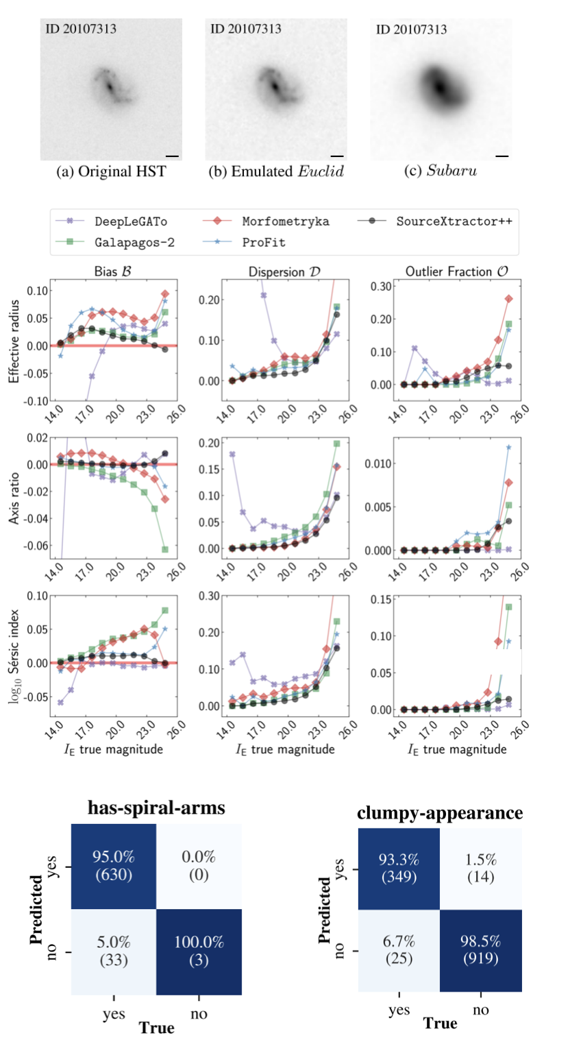
10.4 Active galaxies across redshift
Active galaxies have compact regions at their centres with characteristics indicating that their luminosity is not produced by stars but is the result of the accretion of matter onto a supermassive black hole (SMBH) at the centre of its host galaxy. While all local massive galaxies show some level of AGN activity (Sabater et al. 2021), phenomenology caused by a high accretion rate onto the central black hole is seen in less than 10% of massive galaxies, and is thought to be short-lived (500 Myr to a few Gyr).
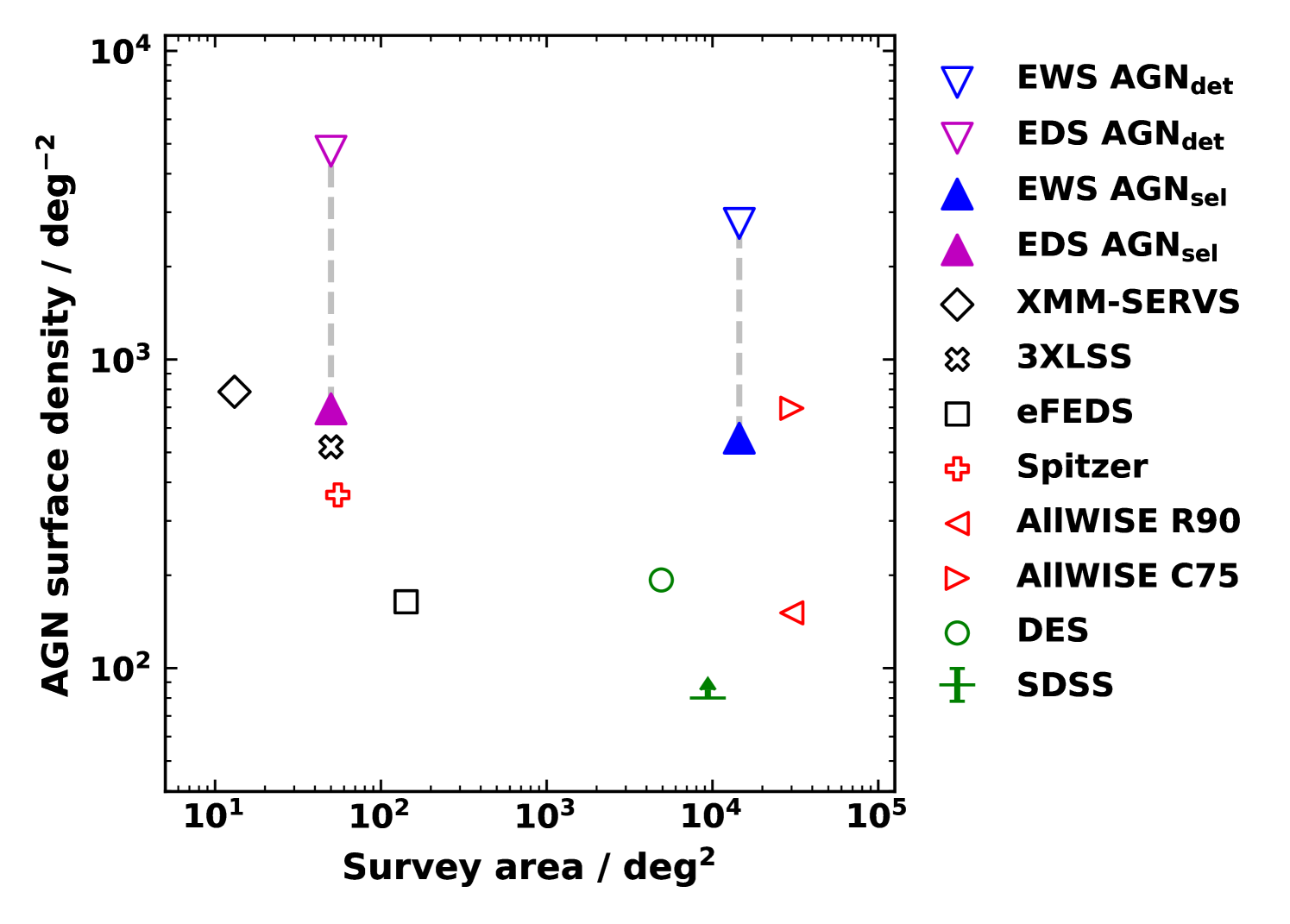
Type 1, or unobscured AGN, typically show broad emission lines () and power-law continuum emission originating from the accretion disk, while Type 2, or obscured AGN, typically show extreme emission line ratios compared to the normal galaxy population and continuum emission with host galaxy features. In orientation-based unification models (e.g. Antonucci 1993; Urry & Padovani 1995; Netzer 2015), Type 2 AGN have been described as obscured Type 1 AGN with the broad-line emitting region and accretion disk being hidden behind a partially opaque torus. According to this simple scheme, Type 1 and 2 AGN should have similar distributions in terms of redshift, luminosity, host galaxy properties, and black hole mass. By contrast, in AGN evolutionary scenarios (e.g. Hopkins et al. 2008; Hickox et al. 2009), obscured Type 2 AGN may represent an earlier evolutionary phase compared to unobscured systems, and thus have different physical properties. The transition from obscured to unobscured accretion in AGN is postulated to occur through an outflow phase, during which energetic feedback is deposited in the host galaxy, impacting the formation of new stars (for a review see Harrison et al. 2018). Given their transient nature, comprehensive studies necessitate very large sample sizes to decipher their evolutionary paths, link to their host galaxies, clustering tendencies, and large-scale environments.
The unique combination of spatial resolution, depth and wide area coverage of Euclid will allow us to explore the AGN population like never before using both photometric and spectroscopic selection criteria. Euclid’s spatial resolution will provide critical observational constraints on AGN morphology and merger rate of their host galaxies. The depth of the NIR observations will allow for the first time the detailed study of Type 1 and Type 2 AGN sub-populations and their co-evolution with galaxies during the so-called ‘Cosmic Noon’ () and beyond. Finally, due to the depth and wide area coverage, rare and extreme states, such as red quasars, will benefit from detailed analysis of their morphologies and large-scale environment.
The most luminous Type 1 AGN, namely quasars, can be identified using Euclid photometry alone or in combination with multi-band coverage from optical surveys, such as LSST. We estimate that () AGN will be detectable (at 5) in at least one Euclid filter in the EWS (EDS), corresponding to a surface density of AGN per square degree (46 open downwards triangles; Selwood et al., in prep.). This large sample will include about 30% Type 1 and 70% Type 2 AGN, based on population studies in the X-rays (Fotopoulou et al. 2016; Merloni et al. 2014). A colour selection using u band in combination with the i, r, or z filter, reaches completeness and purity 81% (77%) and 92% (91%) for the EWS (EDS), respectively (Bisigello et al., in prep.). As shown in Fig. 46, this corresponds to a total of () AGN in the EWS (EDS) identified as AGN, by using Euclid and LSST colours (filled triangles). This simple colour selection will provide quasar surface densities that are better or en par with current AGN surveys, from X-rays (e.g. XMM-SERVS, Chen et al. 2018), optical (e.g. DES Yang & Shen 2023) and mid-infrared (e.g. WISE 75% completeness – C75, Assef et al. 2018). On the other hand, the identification of Type 2 AGN is challenging with Euclid and optical filters alone. Longer wavelength observations, in combination with more sophisticated methods, are therefore necessary.
The identification of AGN in Euclid will also rely on spectroscopic data. Type 1 AGN will be classified through broad emission-line detection, while Type 2 AGN will be identified by using the narrow emission-line [N ii]6584/ versus [O iii]5007/ diagnostic diagram, called the Baldwin–Phillips–Terlevich (BPT) diagram (Baldwin et al. 1981). A notable challenge for the BPT AGN identification using Euclid spectroscopy is the limited spectral resolution (), leading to the blending of key emission lines ( and [N ii]6548,6584) and a restricted availability of diagnostic narrow emission lines in specific redshift ranges within the EWS and EDS (Euclid Collaboration: Lusso et al. 2023).
With Euclid we will use BPT diagrams to classify and characterise Type 2 AGN within the narrow redshift range () in the EWS (EDS), which corresponds approximately to the peak of star-formation activity. Additionally, bright Type 2 AGN will be identified through the detection of high-ionisation emission lines, such as [Ne v]3426 (Mignoli et al. 2013) at and C iv at in the EDS (e.g. Mignoli et al. 2019). Furthermore, spectroscopic redshifts will be available for millions of Euclid AGN. We expect to determine spectroscopic redshifts for around 90% of the Type 2 AGN in the redshift range down to an emission line flux of about for the integrated H [N ii], whilst the same redshift completeness percentage occurs for an emission line flux more than a factor of two higher for Type 1 AGN, namely (Euclid Collaboration: Lusso et al. 2023).
Euclid’s exceptionally extensive AGN data set presents a unique opportunity to constrain the LF of AGN in the near-infrared, over larger magnitude and redshift ranges, and larger area than previously employed to generate NIR galaxy LFs (Bell et al. 2003; Cirasuolo et al. 2007). The AGN LF and its evolution with time are key observational quantities for understanding the origin of SMBHs and accretion onto them (Aird et al. 2013; Shankar et al. 2013; Schulze et al. 2015). Additionally, the measurement of the SMBH mass serves as a key parameter for studies aimed at establishing scaling relations between black holes and host galaxy properties. These scaling relations are vital for testing black hole feedback mechanisms (e.g. Steinborn et al. 2015) and cosmological hydrodynamical simulations of structure formation that investigate the relationship between galaxy and black hole growth (e.g. DeGraf et al. 2015). The AGN LF and the SMBH demography (Euclid Collaboration: Lusso et al. 2023) will be important observational products of Euclid, along with the AGN clustering, which links the evolution of growing SMBHs and the large-scale cosmic structure (Allevato et al. 2019), and the study of AGN close pairs and galaxy mergers.
10.5 Galaxies and quasars in the epoch of reionisation
Euclid’s combination of optical and NIR instruments makes it ideally suited for identifying galaxies and quasars at high redshifts, taken here to be . Whilst other telescopes can reach these distant redshifts, most notably HST and JWST, Euclid has the advantage that it covers a large area of the sky and therefore can find rarer but brighter sources. The data from Euclid will be sufficiently deep such that it will probe into the EoR whereby all sources at these redshifts will exhibit Ly breaks (Gunn & Peterson 1965), redshifted to an observed wavelength of . Such sources would be detectable in Euclid’s NISP images and grism spectra but will be VIS dropouts, so they could potentially be identifiable using Euclid data in isolation. The difficulty is that the vast majority of optical dropouts are not high-redshift sources, so the reliable selection of these sources represents a significant data analysis challenge (even with access to external data sets); however, the potential Euclid science return from high-redshift galaxies and quasars justifies this effort.
Euclid will cover 50 deg2 to depths of about 26.4 AB magnitudes ( point source limit) in the NIR filters in the EDS fields, which means that it probes a unique parameter space in the selection of galaxies. Previously, space-based NIR telescopes have been limited in their ability to select the brightest and hence rarest sources due to their small FoVs: the Wide Field Camera 3 (WFC3) on HST has an FoV of 4.5 arcmin2 and the Near-InfraRed Camera (NIRCAM) on JWST has an FoV of 9.7 arcmin2. Even with large efforts to produce mosaics, these cover . Hence, while the study of ultra-high-redshift galaxies was undoubtedly revolutionised with the deep NIR surveys of HST and JWST, which allow galaxy candidates to be identified up to –13, the identified galaxies are typically limited to (with being the knee in the rest-frame UV LF; see review by Stark 2016). In the traditional ‘dropout’ formalism, galaxies will be selected with Euclid via the Lyman-break as dropouts at , -dropouts at , and -dropouts at , and Euclid can in principle detect sources up to because the band extends up to 2 . Importantly, the higher resolution of the Euclid imaging will aid in the identification of the main contaminants, brown dwarfs (cf. Sect. 10.1), since the galaxies are expected to be resolved at these bright magnitudes. Moreover, contamination fractions from galaxies can be reduced from up to 40% to less than 5% with the inclusion of deep optical photometry, such as LSST (Euclid Collaboration: van Mierlo et al. 2022).
These luminous galaxies provide signposts to the most ionised regions of the neutral IGM at , while also representing a challenge to theoretical models and being key candidates for multi-tracer follow-up, for example with Atacama Large Millimeter/Sub-millimetre Array (ALMA) and JWST. Recent results from JWST (e.g. Naidu et al. 2022; Donnan et al. 2023; Finkelstein et al. 2023) have revealed a surprising abundance of luminous sources, of which several have shown unusual spectral features (e.g., GNz11; Oesch et al. 2016; Bunker et al. 2023). These results highlight the huge potential of Euclid-selected high- sources in understanding the earliest stages of galaxy formation and reionisation.
Much of this work in the deep fields will be aided by observations from the Cosmic Dawn Survey (Sect. 4.4), which provides matching depth -band from CFHT, -bands from HSC on Subaru, and 3.6 and 4.5 from Spitzer/IRAC as described in more detail in Sect. 4.4. The science goals of this survey are primarily focused on the high-redshift Universe, but will also facilitate many aspects of legacy science for the Euclid mission. Leveraging the deep wide area data from the Cosmic Dawn Survey will provide robust measurements of the galaxy stellar mass function to and the UV luminosity function to . Other science goals include mapping the topology of reionisation, studying the formation of large-scale structure, quantifying the prevalence of high-redshift protoclusters, and characterising the first quenched galaxies. The survey data have immediate value for studying galaxy formation and evolution, and that legacy value will only increase as more data are collected.
Previous work on smaller scales shows the potential of Euclid discoveries. Degree-scale ground-based surveys from UKIRT and VISTA have provided the first view of the LF at for –, showing an excess of sources over the predictions of HST surveys and revealing an apparent lack of evolution in the number density of the brightest sources (e.g. Bowler et al. 2020; Harikane et al. 2022). With the unique combination of space-based, wide-area, deep NIR imaging provided by Euclid, the number of rare luminous galaxies will be increased by factors of 100–1000 over current samples, providing key constraints on the bright end of the LF. Integrating the current best-fit LFs leads to predictions of thousands of sources from the deep fields, down to an absolute UV magnitude of . This allows the shape at the bright end – which depends sensitively on astrophysical effects such as dust, scattering, and lensing – to be unambiguously determined. If the slope of the bright end continues as a power law beyond observational limits, there is the possibility of detecting a substantial number of extremely bright galaxies with NISP within the EWS (approximately 2000 versus 50 for a double-power law or Schechter function, respectively, at ; Bowler et al. 2017). These additional objects will not only be useful for deriving the LF, but can be used to study the structures, stellar masses, and star-forming properties of these early systems and to compare them to lower redshift systems, as well as with galaxies at lower masses studied with HST and JWST.
High-redshift quasars are much more luminous than comparably distant galaxies (and, unlike -ray bursts, are non-transient) and so are among the most useful probes of the high-redshift universe. As described in the review by Fan et al. (2023), spectroscopic observations of high-redshift quasars probe the growth of the first SMBHs, provide several unique constraints on cosmological reionisation, and also give a record of the evolution of elemental chemical abundances. Luminous high-redshift quasars are expected to be extremely rare: while the redshift range is reasonably well explored, with approximately 300 quasars known, just eight bright quasars have so far been spectroscopically confirmed to be at (Fan et al. 2023), along with some more speculative fainter detections at even higher redshifts using JWST (Maiolino et al. 2024; Bogdán et al. 2024). It is in this regime that Euclid should be able to make a transformational contribution, thanks primarily to the large area coverage of the EWS (Sect. 4.1). The headline prediction given in Laureijs et al. (2011) was that Euclid imaging data would be expected to include 55 quasars brighter than , sufficient to completely revolutionise this field. Euclid Collaboration: Barnett et al. (2019) then presented a more realistic simulation, which explored the impact of a range of contaminants (M, L, and T dwarfs, as well as early-type galaxies at ), different selection methods, the availability of external optical data (from LSST), and uncertainty about the evolution of the quasar LF.
While these simulations showed that the Euclid data should be able to produce complete high-redshift quasar samples to a greater depth of (particularly if it is possible to cross-match to LSST optical data, this is outweighed by the steeper decrease in quasar numbers with redshift found by Jiang et al. (2016). So the realistic predictions from Euclid Collaboration: Barnett et al. (2019), given in full in Table 3 of that paper, are broadly that the EWS photometry343434It is also possible that the brightest high-redshift quasars could be identified from the Euclid grism spectra directly. Unfortunately, the simulations described by Roche et al. (2012) are no longer relevant because of the subsequent reduction in the capabilities of the grisms, and no updated studies of this possibility have been published to date. will yield approximately 100 robust quasar candidates with , around 25 quasars beyond the current record of (Bañados et al. 2018; Yang et al. 2020; Wang et al. 2021), and perhaps 10 quasars at .
While the Euclid photometry will be necessary to identify (candidate) quasars, confirmation and characterisation will (in contrast to most other projects described in this paper) come primarily from external follow-up observations. Most important will be NIR spectroscopy; hence there is a particular utility to finding the brightest sources with , corresponding to . Even one such detection at (plausible in DR1) would represent major progress in this field; the full EWS should yield a well-characterised population of quasars out to at least , with the observational frontier possibly pushed back as far as .
10.6 Galaxy evolution and environment
While it is largely agreed that the cosmic environment in which a galaxy evolves strongly correlates with its measured properties (e.g. Darvish et al. 2017), we still need to understand all the physical processes that drive its evolution as well as their relative importance. Dressler (1980) showed that, at least in the local Universe, galaxies in denser environments are more likely to be elliptical galaxies, whilst systems found within regions of lower density are generally galaxies with spiral and irregular morphologies. Furthermore, in the local Universe, with the exception of radio-bright galaxies that preferentially reside at the centres of clusters (see Magliocchetti 2022, for a review), AGN are observed to avoid massive structures (e.g. Popesso & Biviano 2006).
A wide diversity of other properties are observed to correlate with various measures of environment as well. For instance, on average, high-density regions are mostly populated by redder, brighter, more metal rich, and less star-forming galaxies, while the opposite is true for low-density regions (e.g. Kauffmann et al. 2004; Blanton et al. 2006; Winkel et al. 2021). Additionally, ‘green valley’ galaxies, likely to be transitioning from star-forming to quiescent phases, have a lower specific star-formation rate in groups and clusters than in the field (e.g. Jian et al. 2020). Another example is the positive (negative) correlation between the star-formation rate (H i gas deficiency) of galaxies, at fixed mass, and their distance to the closest filamentary structure (Malavasi et al. 2017; Laigle et al. 2018; Kraljic et al. 2018; Gouin et al. 2020, Crone Odekon et al. 2018), or the recent evidence that galaxies that are strongly connected to the cosmic web form fewer stars and are more pressure supported than those that are weakly connected. (Kraljic et al. 2020). Furthermore, a bimodality in the central surface brightness of disks is found for galaxies in voids, filaments and knots, but not in sheets (Sorce et al. 2016). All these findings seem to hold at least out to (e.g. Cucciati et al. 2010; Jian et al. 2020).
At higher redshifts the situation is less clear, although there seems to be increasing evidence for a reversal of at least some of the scaling relations mentioned above. As an example, it has been found that at –2 more AGN reside within dense regions than in the field (e.g. Martini et al. 2013). However, the exact details of the processes leading to such observed correlations at are still unknown. Evolutionary paths followed by galaxies are extremely complex, especially because several processes are at play in an intertwined way. For instance, McGee et al. (2009); De Lucia et al. (2012); Verdugo et al. (2012) and Sarron et al. (2019) showed that galaxies are probably preprocessed in groups (filaments) before falling into clusters where they finish their transition to passive states.
Given its extremely wide area coverage, Euclid will probe all environments in which galaxies are found, even the most extreme ones, over the widest redshift range to date. Indeed, it will be able to measure properties (such as redshifts, stellar masses, star-formation rates, presence and relevance of a central AGN) for billions of galaxies in regions of varying density out to and, in the three deep fields, even out to .
In order to exploit the exquisite quality of Euclid data for environmental studies, we have developed several codes for the reconstruction and characterisation of the observed density field traced by Euclid galaxies at all scales. These all deal with the search of overdense structures such as high- clusters and protoclusters. We also optimised existing codes for the detection of cosmic filaments (e.g. Sousbie 2011) in order to work with both photometric and spectroscopic samples. These codes will complement those already used for the detection of voids (e.g. VIDE, Sutter et al. 2015 and Contarini et al. 2022) and clusters (AMICO and PZWav, Euclid Collaboration: Adam et al. 2019), allowing the reconstruction and investigation of the full density field at all scales. This will permit us to shed light on the link between galaxy and AGN formation and evolution and their environments out to .
Furthermore, the codes developed for the investigation of the clustering properties of Euclid galaxies both in configuration space (two- and three-point correlation functions) and in Fourier space (power spectra and bispectra, cf. Sect. 7.7.1) will also be used to relate the properties (stellar mass, colour, luminosity, star-formation rate, metallicity, star-formation history, black hole type, accretion, luminosity, etc.) of the galaxies and AGN observed by Euclid with the LSS they trace. This will permit the establishment of a direct connection with the dark halos inhabited by these sources, via the so-called bias function (e.g. Mo & White 1996; Scoccimarro et al. 2001).
10.7 Star-forming galaxies across time
The combination of photometry and spectroscopy will enable detailed investigations into the physical properties of star-forming galaxies, such as stellar populations, star-formation rates, and dust attenuation, as well as their evolutionary processes and the interplay between star formation and black hole accretion at the peak of AGN activity and star-formation history, during Cosmic Noon.
In the EWS Euclid will map 2000–4800 H emitters per deg2 in the redshift range at a flux limit of , totalling 28–67 million sources in the EWS, while in the EDS we will amass about 32 000–48 000 H emitters per deg2 (i.e. a total of 1.6–2.4 million) at a flux limit of , in the broader redshift range enabled by the addition of the blue grism (Pozzetti et al. 2016). For these galaxies it is not only possible to obtain robust spectroscopic redshifts, but we will also be able to study a wide range of properties. First of all, the star-formation rate (SFR), which can be estimated from the intensity of the emission line (e.g. Kennicutt 1998b), corrected for dust attenuation using /, when is available or statistically otherwise: with such a sample of tens of millions of emitters we will be able to analyse in detail the tight correlation between SFR and stellar mass, the so-called galaxy main sequence (MS), down to a few at in the EWS, as shown in Fig. 47. In particular, with the EWS sample we will be able to probe the most massive part () of the MS with unprecedented statistics at these redshifts, and help provide the physical explanation for the observed turnover in the MS shape and its evolution (e.g. Popesso et al. 2023). Additionally, the EDS will allow us to explore the fainter end of SFR-stellar mass space. Moreover, thanks to the wider wavelength range due to the availability of the blue grism, multiple spectral lines will be available for individual galaxies (e.g. , [O iii]5007, and [O ii]3727), enabling us to recover dust attenuation and gas-phase metallicities, and to put solid constraints on a variety of scaling relations (e.g. the fundamental metallicity relation and mass-attenuation Maiolino & Mannucci 2019). In the EWS we expect to find about 440 [OIII]5007 emitters per deg2 (resulting in a total of about over the entire EWS area) in the range (Bagley et al. 2020). Finally, a complementary sample of emitters would also be mapped at low redshift (), similar to Cleri et al. (2022) with HST grism G141.
Euclid photometric information, complemented by ground-based data, will also be used to derive the physical properties of galaxies (Euclid Collaboration: Bisigello et al. 2023). In particular we will be able to classify galaxies from their photometric SED (Bisigello et al. 2020) and compute the stellar mass function (SMF) of galaxies of different classes to derive its differential evolution and infer the history of cosmic mass assembly. The enormous EWS area will enable the study of the evolution of the number density of rare populations, like massive star-forming galaxies, in order to relate them to the mass growth and buildup of passive galaxies, while assessing the contribution due to mergers, thanks to the exquisite morphological information that the Euclid high resolution will provide (cf. Sect. 10.3). By comparing the SMFs of galaxies classified with different methods (i.e. using their morphology or colours), it will also be possible to understand the timescale of the morphological transformation and stellar population ageing (e.g. Pozzetti et al. 2010) that lead to the present-day galaxies and to derive constraints on the quenching mechanisms (Peng et al. 2010) responsible for turning off star formation.
The combination of physical and morphological properties will provide constraints on the size-mass relation of blue star-forming galaxies and insights on the connection between the compactness of galaxies, their light profiles, and the efficiency of the star-formation process, leading to an understanding of the range of properties of the blue cloud galaxies quenched by internal mechanisms (Hamadouche et al. 2022). To explore the parameter space sampled by the EWS and EDS even further, we will consider samples of galaxies sharing similar properties, for instance by reducing the high-dimensional photometric space of colours and fluxes with machine-learning algorithms (e.g. SOMs, as in Davidzon et al. 2022, see also Sect. 7.6.1). The spectra of these groups of galaxies can then be analysed with stacking techniques to improve the signal and eventually study the MS at 0.91.82 at SFRs as low as in the EWS, and in the EDS. Similarly, SED fitting will be performed on the photometric composite SEDs with high S/N to analyse the physical properties and their evolution especially of faint galaxies. Taking advantage of the 3-dimensional distribution of galaxies (see Sect. 10.6), we will study how the physical properties of galaxies depend on the environments they inhabit.
The source-subtracted cosmic infrared background (CIB) fluctuations uncovered in deep Spitzer data (e.g. Kashlinsky et al. 2005, 2012) are coherent with the unresolved cosmic X-ray background (CXB; Cappelluti et al. 2013; Mitchell-Wynne et al. 2016; Cappelluti et al. 2017; Li et al. 2018), which could be caused by a new population (Helgason et al. 2014) containing a fraction of black holes in excess of what appears in the known galaxy populations. As discussed in Kashlinsky et al. (2018), Euclid will play an important role in directly resolving the nature of the CIB at near-IR wavelengths, because the source-subtracted CIB measurements in the three Euclid near-IR bands over the EWS can be cross-correlated with the unresolved CXB from eROSITA to constrain model predictions (Kashlinsky et al. 2019).
In the far-IR, a statistical characterisation of star-formation processes across cosmic epochs can be obtained from a joint analysis of Euclid data and maps of the far-IR CIB, which probes the unresolved emission of dusty star-forming galaxies since the epoch of reionisation (Dole et al. 2006). Maps of the far-IR CIB can be extracted from multi-frequency CMB observations through component separation or from direct observation at relevant frequencies, such as those of Herschel, which is, however, hard to extract due to residual Galactic foreground contamination in far-IR CIB maps (Planck Collaboration XVIII 2014; Maniyar et al. 2019; McCarthy et al. 2023). Instead, the cross-correlation of CIB maps of Planck, Herschel, or future ground-based instruments (such as the Cerro Chajnantor Atacama Telescope) with the Euclid observables (galaxy or QSOs clustering and cosmic shear) can be used to constrain models of star-formation history, its efficiency across time, and the connection to host halo mass and environment (Jego et al. 2023a, b). Euclid’s NIR images from both the EWS and EDS can be used to create background maps (after masking the detected sources) and directly cross-correlating with CIB maps from the same external sources to extract additional complementary information (Lim et al. 2023).
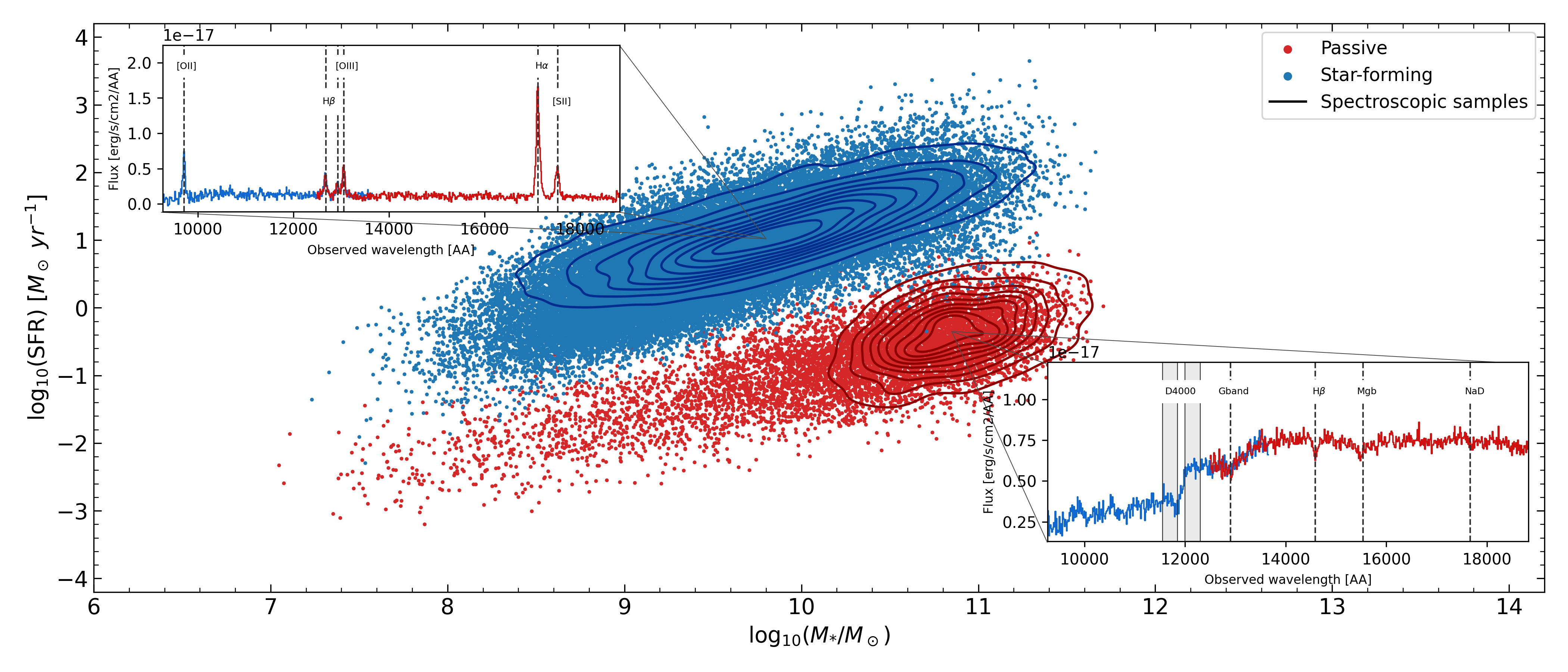
10.8 Passive galaxies and galaxy quenching
Massive (), quiescent galaxies are key systems for understanding galaxy formation, but they are rare and it is therefore challenging to assemble large samples. Euclid spectroscopy can play a unique role in studying these systems in the EDS at high redshifts. Indeed, due to the rapid decline of their number densities at (Weaver et al. 2023), finding and observing over the widest possible redshift range is a crucial yet difficult task.
Much work has been done out to , but the peak of star-formation activity and the assembly of passive galaxies is at (Ilbert et al. 2010, 2013; Madau & Dickinson 2014). The study of the number densities of massive passive galaxies at high redshift – that is the galaxy SMF– is crucial for understanding how the evolution proceeds from star-forming to passive galaxies, that is when galaxies are quenched, and when and how they assemble their mass, which is still a challenge for models of galaxy formation. The EDS with the BG will be truly unique for finding and spectroscopically identifying, at the continuum limit (), the rarest and most massive quiescent galaxies at , with (11). The evolution of the luminosity and mass functions of passive galaxy types can be followed in different environments (e.g. Cucciati et al. 2016, show the possibility to measure galaxy environments in the EDS over the redshift range , see also Sect. 10.6). Therefore, the Euclid deep BG data can be used to probe the assembly of the red sequence out to .
The BG provides a fundamental complement to the RG for the identification of a large sample of quiescent galaxies based on the identification of the Balmer or D4000 break. We consider for the BG the wavelength range 0.926–1.366 , and 1.206–1.892 for the RG (50% peak transmission wavelengths) and a reference EDS area of 50 deg2. The blue limit of , around 0.926 , allows us to detect the break starting at and up to , while the RG allows its detection only in the redshift range , where the expected number of passive galaxies is significantly smaller.
To obtain quantitative estimates of the expected numbers of passive galaxies, we have used the COSMOS2020 catalogue (Weaver et al. 2022) to derive the number density of passive galaxies expected for different limits. We have selected passive/quiescent galaxies using the colour-colour selection versus and derived the redshift distributions for different limits. At the limit, about 5000 passive galaxies will be detectable at within the sensitivity limits of NISP continuum spectroscopy over 50 square degrees at =21 in the EDS, and over 30000 at =22.
The red grism extends the possibility of detecting passive galaxies, through the D4000 detection at , but only at . A typical example is shown in Fig. 47. Keeping in mind the drop in the number of passive galaxies above , the importance of having a blue grism is clear, since it allows for the detection of more than massive quiescent galaxies with and approximately () galaxies with (23) in 50 deg2. These numbers are to be contrasted with the several hundreds of spectroscopically confirmed objects in the RG.
Euclid will not only provide a huge sample of passive/quiescent galaxies compared to what has been available before, but will also be fundamental for finding and spectroscopically identifying the rarest and most massive passive galaxies () with unparalleled statistics. This is because their number density (10–100 deg-2) makes their identification difficult with NIR instruments with a small FoV from space (e.g. JWST or HST), while from the ground strong sky residuals limit the sensitivity (e.g. VLT+MOONS or SUBARU+PFS). Only JWST can compete with Euclid in this area, but will provide much smaller samples.
At high redshift (), which is the most active period of galaxy assembly, but where ground-based spectroscopy is inefficient, Euclid will truly revolutionise the field and will be a unique facility for galaxy evolution analysis. The large number of passive galaxies provided in the EDS with the BG plus RG can be used to follow in detail the growth of this fundamental class of rare galaxies that remain a challenge for models of galaxy formation.
The detection of passive galaxy spectroscopic pairs could be used to evaluate the dry galaxy merger contribution to the assembly of massive passive galaxies. Galaxy mergers are, indeed, an essential part of the evolution of galaxies in any hierarchical cosmological model, but current observational constraints on the merger rate cannot distinguish between models due to the small existing samples (Duncan et al. 2019; Conselice et al. 2022).
Euclid’s BG plus RG spectra in the EDS will allow us to study, using spectral fitting techniques, the evolution of massive and passive galaxies in terms of the physical properties of their stellar populations (such as ages, metallicities, dust content, and velocity dispersions), with extraordinary statistics compared with present and future ground-based data sets. High-S/N () spectra are needed to reconstruct physical properties (see, e.g. Citro et al. 2016) with high accuracy; we can perform such a study on the brightest subsample or on stacked spectra.
10.9 The galaxy-halo connection from gravitational lensing
Science with galaxy-galaxy lensing (GGL) focuses on the relation between galaxies, their baryonic properties (luminosity, stellar mass, etc.), and their dark matter halo properties (mass, density profile, shape, and environment), that is, the galaxy-halo connection. We will exploit the precise lensing signal around foreground galaxies with the aim to constrain the halo mass as a function of luminosity and/or stellar mass and to distinguish between central and satellite galaxies. The lens samples will be split by various properties, such as rest-frame colour, redshift, and size to explore the variation in the stellar mass-halo mass relation (SHMR) as a function of galaxy type and to quantify the evolution of this relation up to . The Euclid data should be able to constrain this from the GGL signal alone, but the analysis may need to include additional priors, for instance from the luminosity or stellar mass function. For this, we will use lens samples obtained from Euclid photometric redshifts, from large ground-based spectroscopic surveys such as DESI (DESI Collaboration et al. 2024), as well as from Euclid spectroscopy. In the particular case of NISP emission-line galaxies detected in spectroscopy with Euclid, we will model their HODs, and use this information to build mock galaxy catalogues for the cosmological analysis. As shown in Fig 48, although at quite high redshift, we expect a GGL signal of in five redshift bins in the range and down to 1 arcmin scale.
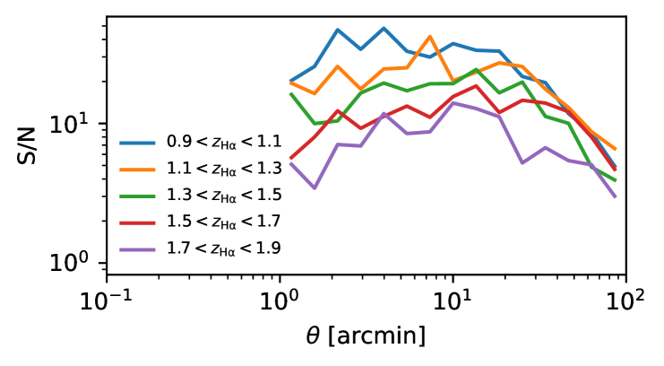
We also anticipate HOD constraints with galaxy-galaxy-galaxy lensing (G3L; Schneider & Watts 2005; Simon et al. 2008), which encompasses the correlation between the positions of pairs of lens galaxies with the shear of a source galaxy (shear-lens-lens G3L), and the correlation between the shears of pairs of sources with the position of individual lenses (shear-shear-lens G3L). G3L depends on HOD parameters in a way that is different than for the second-order statistic GGL. Hence, similarly to HODs for cosmological inference (see Sect. 9), combining GGL and G3L can reduce parameter degeneracies in the HOD that define the occupancy of central and satellite galaxies (such as minimal halo masses for galaxy formation and satellite fractions) and improve constraining power. Moreover, G3L can probe the correlations between different lens samples, for example, red-sequence and blue-cloud galaxies (Linke et al. 2022).
While G3L has been detected in smaller and shallower ground-based surveys (Simon et al. 2013; Linke et al. 2020), Euclid will provide an immense improvement in the S/N due to its larger area and higher galaxy number density. This is particularly important for the shear-shear-lens G3L, whose signal is about two orders of magnitude lower than shear-lens-lens G3L (Simon et al. 2013).
Measuring the radial mass density profiles of galaxies is important because baryonic cooling and feedback effects likely alter this from the standard dark matter-only halo density profile (Sonnenfeld et al. 2018). Empirically determining the profile is critical for both understanding galaxy formation and for its impact on cosmology. This is possible through careful measurement and modelling of the excess surface density, derived from the GGL tangential shear. Moreover, by combining weak and strong lensing, we can obtain tight constraints over the whole profile, provided that the selection function for strong lenses can be quantified.
Measuring the flattening of the dark matter halo is also possible with GGL. We will use the quadrupole moment of the tangential shear referenced to the major axis of the light, correcting for spurious signal caused by cosmic shear, large-scale alignments between galaxy shapes, and the tidal field of the matter, as well as additive PSF systematics. The measurements will be conducted for lens galaxies split, for example, according to colour or luminosity/stellar mass, to facilitate the comparison to predictions from simulations. With GGL alone, it is not possible to measure the ellipticity of a halo independently from the misalignment between the orientation of the halo and its central galaxy (e.g. Bett 2012). To break this degeneracy and so constrain the halo ellipticities, we will combine GGL with shear-shear-lens G3L, which is sensitive to the overall halo ellipticity (Simon et al. 2012; Adhikari et al. 2015; Shirasaki & Yoshida 2018).
Finally, we will use GGL to assess the link between galaxy content, galaxy halos, and their large-scale environments, extending the work described in Sect. 10.6. For example, we expect that satellite galaxies will have tidally stripped halos (e.g. Sifón et al. 2018), which will become increasingly truncated as they spiral into their host group or cluster. Moreover, we will explore larger-scale structures such as filaments between galaxies (Epps & Hudson 2017), a form of G3L (lens-lens-shear), and weak lensing by cosmic voids and the galaxies within them.
10.10 Clusters as testbeds for astrophysical processes
Clusters of galaxies are powerful testbeds for various astrophysical phenomena, from AGN heating to tidal stripping; this is because almost all of the matter in them can be probed. The dark matter is so densely concentrated that it can be traced by strong and weak gravitational lensing (e.g. Bradač et al. 2005; Umetsu et al. 2016). The intracluster medium is visible through X-ray and sub-millimetre observations and carries information about the thermal and chemical enrichment history (e.g. Voit 2005). Member galaxies, although representing a minor contribution to the total and baryonic mass budget, trace the dynamics of the system and retain memory of the formation and evolutionary path in their morphologies and colours. Additionally, the diffuse glow of intracluster light, situated between the cluster galaxies, enables the tracking of stars that have been stripped from previous galaxy mergers and interactions (Montes 2022). However, due to the rarity and size of clusters, our knowledge of their physical properties is limited to relatively small samples, primarily focused on core regions and predominantly at .
Euclid will be transformational, since it only needs to be combined with a probe of the gas (e.g. from eROSITA, XMM-Newton, Chandra, Planck, ACT, or SPT) to provide a comprehensive view of the state of the clusters. The high-resolution VIS images enable the mass distribution to be mapped using weak lensing, the combination of the spectra and galaxy positions will reveal the dynamical state of the cluster, and the low sky-background in the NIR means intracluster light can be observed out to .
Euclid will be able to measure the weak lensing masses of nearly massive clusters with a relative uncertainty of less than 30% (Euclid Collaboration: Sereno et al. 2024, also see Köhlinger et al. 2015). Weak lensing analyses of individual clusters or stacked samples will accurately probe the mass distribution from the inner and virial region, with accurate measurements of the inner slope and concentration (Sereno et al. 2016; Euclid Collaboration: Giocoli et al. 2024), to the cluster boundaries and beyond, constraining the splashback radius (the radius at which accreted matter reaches its first orbital apocentre after turnaround) and the infalling region (Umetsu & Diemer 2017; Contigiani et al. 2019; Giocoli et al. 2024), and the correlated matter in the cluster environment (Sereno et al. 2018; Giocoli et al. 2021; Ingoglia et al. 2022).
With the redshifts, the masses, and the dynamical states of the clusters provided by Euclid observations, the properties of the gas and the baryon budget will be readily predicted from theories of gravitational collapse (Voit 2005). Any deviation from these predictions and comparisons with state-of-the-art simulations will be used to quantify the impact of non-gravitational physics such as gas cooling and feedback from supernovae and AGN, as well as to probe hydrodynamical phenomena induced by hierarchical structure formation, such as the process of mass and energy accretion and distribution though shocks, turbulence, and bulk motions (Kravtsov & Borgani 2012), plus the relative importance of cosmic rays and magnetic fields (Brunetti & Jones 2014). These astrophysical phenomena are the reason that the galaxy-halo connection is so complex and our poor understanding of these phenomena limit our ability to constrain cosmology with both primary Euclid probes (see Sects. 2.2 and 8.2.1) as well as with cluster counts.
As mentioned in Sect. 10.2, Euclid will have an unrivalled ability to measure low-surface brightness features in the infrared, with , , and depths of (Euclid Collaboration: Scaramella et al. 2022), which are sufficient to observe intracluster light out to 100 kpc in protoclusters (Werner et al. 2023) and to the splashback radius in clusters to (Gonzalez et al. 2021). Intracluster stars, freed from their host galaxies, are expected to follow the global distribution of dark matter in clusters and may act as a luminous tracer of the dark matter distribution (Montes & Trujillo 2019), which is especially important for the clusters where mass measurements from weak gravitational lensing cannot be made.
10.11 Protoclusters
Galaxy clusters in the local Universe are dominated by elliptical galaxies that were formed in the early Universe at , often in short-lived intense starbursts (e.g. Bower et al. 1992). Therefore, understanding how clusters assembled their mass in the early Universe is of critical importance, because their precursors are expected to contribute significantly to the star-formation rate density at high redshifts (Chiang et al. 2017).
Although different definitions are used in the literature, Overzier (2016) suggests to define a protocluster as ‘a non-virialised structure in the distant Universe that will finally collapse into a typical local galaxy cluster, a virialised system of a mass larger than . Although a common definition is useful in many respects, we acknowledge that the very nature of protoclusters (i.e. being defined based on their future fate) prevents a robust and univocal operational definition.
The study of galaxy protoclusters in the distant Universe has been an emerging research field in the past decade (for a review, see Overzier 2016) and is now reaching maturity, with an increasing number of systematic searches, complemented by serendipitous discoveries. Both the EWS and EDS, together with the exquisite optical/NIR imaging data sets, offer a unique opportunity to search for protoclusters in a systematic way and make a big leap forward in this research field (Böhringer et al., in prep.). To this end, we have developed several tools tailored for the detection of galaxy protoclusters, including fine-tuned variations of the two official cluster-selection algorithms AMICO (Bellagamba et al. 2018) and PZWav (Gonzalez 2014, also see Sect. 7.7.4). All these codes have been applied to real data and Euclid-like simulations to study the properties of protoclusters as they will be observed in the Euclid surveys and to test the synergies with other available data-sets. With such a study we aim to provide guidelines for the detection of these objects, the interpretation of the results, and pave the way for follow-up observations. More generally, we will study both the physical properties of the protoclusters as whole objects, and the properties of their members. This will allow us to make a complete census of protoclusters at several stages of evolution (which will require a careful synergy with theoretical simulations) and to understand and to understand the physics behind the correlation of galaxy properties with environment (see Sect. 10.6).
For the detection of protoclusters we adopt two strategies: (1) a blind search exploring the entire wealth of data; and (2) a search around possible signposts, such as sub-millimetre galaxies (e.g. Planck Collaboration Int. XXVII 2015; Planck Collaboration Int. XXXIX 2016; Calvi et al. 2023) and/or high- radio galaxies (e.g. Kurk et al. 2000; Pentericci et al. 2000). In this way it will be possible to study, with rich statistics, any possible differences and biases between the two methods. For the protocluster detection, we will rely mostly on photometric redshifts, based mainly on optical and NIR imaging (see Sect. 7.6.1). Protoclusters could also be revealed through overdensities in the spectroscopic redshift data, out to using and perhaps also out to through the [O iii]4959,5007 doublet. For specific areas on the sky, far-IR and (sub)mm observations are also available, and we will use these observations to reveal the progenitors of elliptical galaxies dominating local galaxy clusters, the dusty starbursts (for a review, see Alberts & Noble 2022).
10.12 Transient objects
Exploration of the time domain is a rapidly growing area of modern astronomy. In particular, time-domain astronomy in the NIR is an unexplored frontier. Although the majority of the EWS will be visited only once, some fields such as the EDFs and self-calibration field are planned to be observed repeatedly, and hence they can be used to search for transient objects.
Transient surveys in the NIR can identify transients that are obscured by dust absorption. It has been suggested that a significant fraction of transients, such as supernovae (SNe) and tidal disruption events (TDEs), have been missed by optical transient surveys because of strong absorption in their host galaxies (e.g. Kool et al. 2018; Panagiotou et al. 2023). Measuring the rates of dust-obscured transients will allow us to estimate the true event rates of transients that are essential information to uncover their nature. In addition, some transients are known to be intrinsically bright in NIR and such transients can be explored by Euclid. For example, the extragalactic infrared transient survey conducted by Spitzer revealed that there is a population of unusual infrared transients without optical counterparts (Kasliwal et al. 2017). Thanks to the combination of simultaneous VIS and NISP data, Euclid will be able to carry out a census of transients that are intrinsically luminous in NIR in nearby galaxies to understand their origins.
NIR transient surveys also allow us to discover high-redshift transients. For example, Euclid can discover hundreds of Type Ia SNe at , which could lead to a significant improvement in cosmological parameter estimation if Euclid can perform a dedicated transient survey for 6 months (Astier et al. 2014). Although such a survey is not currently planned, such a dedicated transient survey could be conducted with Euclid if there is time available later in the mission. However, even with the current survey plan, long-lasting luminous transients, such as superluminous SNe and pair-instability SNe, can be discovered out to in the EDFs (Inserra et al. 2018; Moriya et al. 2022). High-redshift superluminous SNe and pair-instability SNe allow us to constrain properties of massive stars (expected to be the progenitors of such SNe) at high redshifts (Moriya et al. 2022; Tanikawa et al. 2023). High-redshift superluminous SNe may also provide additional cosmological parameter constraints (Inserra et al. 2018).
As an indication of the expected numbers of SNe detectable with Euclid, the weekly observations of the self-calibration field (with an area of approximately ) obtained during the PV phase can yield around 40 Type Ia SNe discoveries, of which about 10 are expected to be at . A similar number of core-collapse SNe is also expected to be discovered. During regular operations, the self-calibration field will be observed monthly. Such long-term monthly observations over the full duration of the survey should enable the discovery of around 500 Type Ia SNe at and around 200 core-collapse SNe at . In addition, up to dozens of superluminous SNe and pair-instability SNe out to may be discovered during the long-term self-calibration field observations, depending on their unknown event rates.
An example of an early Euclid discovery of a transient object is shown in Fig. 49. The object with coordinates , (J2000.0) was discovered in Euclid observations of the COSMOS field taken on 21-23 November 2023. The object, a likely SN, brightened significantly during this period, enabling a clear detection in difference images. Subsequent analysis shows that the object is also clearly detected in the three Euclid NIR bands. Given that there is no previously known transient reported at this position, this is a new discovery by Euclid and it is officially named as AT 2023adqt. The host galaxy (SDSS J095940.08+023554.6) has a spectroscopic redshift of (Knobel et al. 2012). Photometry of the transient object yields a brightness of , , and on 23 November 2023. Its optical to NIR colours are consistent with the rise of a SN at the same redshift, although at this stage it is not possible to determine the SN type. The clear detection and deep NIR photometry, enabling detection even when significantly far from peak brightness, demonstrate Euclid s power for the detection and study of transient objects.
Euclid can also provide important information on transients discovered by the LSST (Guy et al. 2022). As the Euclid survey fields overlap with some LSST fields, some transients are likely to be observed by both Euclid and the LSST. In such a case, Euclid can provide complementary NIR photometry information to LSST. Such NIR data can be used to constrain dust production in and around transients, for example. The joint detection of thousands of Type Ia SNe by Euclid and LSST would provide a valuable contribution to our understanding of the impact of dust on Type Ia SN cosmology (Bailey et al. 2023). Euclid will also provide some spectroscopic measurements of SNe after scene modelling (e.g. Lezmy et al. 2022). For transients discovered by LSST and other facilities, the EWS and EDS can provide essential information such as morphology, infrared photometry, and spectroscopy of their host galaxies. Furthermore, red supergiant progenitors of Type II SNe discovered by LSST or other transient surveys may be identified in the Euclid images taken before their explosion.
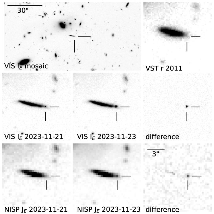
10.13 Demographics of cool exoplanets
From 2027 the NASA Roman mission is expected to undertake the Roman Galactic Exoplanet Survey (RGES, Penny et al. 2019), a statistical census of the cool exoplanet regime using the microlensing effect. The cool exoplanet census will be pivotal for testing planet formation models (Burn et al. 2021), and the RGES census will complement that of hot exoplanets obtained by Kepler (Borucki et al. 2010). RGES is the key science driver for the Galactic Bulge Time Domain Survey (GBTDS), one of the three Roman core community surveys that will each occupy around of the first 5 years of Roman mission.
The RGES is designed to find around 1 400 cool exoplanets down to the mass of Mars (Penny et al. 2019), and to be able to make direct mass measurements for at least half of its sample. Direct planet mass measurements can be achieved through a number of approaches, including: direct measurement of the lens host flux; measurements of finite-source magnification effects in the lightcurve; and measurements of PSF distortion arising from relative proper motion between the foreground lensed host and background magnified source star. Together with the event duration, such measurements provide the means to break what would otherwise be a three-way degeneracy between the planet mass, distance, and transverse speed.
However, many Roman events will have insufficient data to fully break the mass-distance-speed degeneracy, and others may have relatively poor precision due to the challenging measurement of lens-source relative proper motion. Due to the very close alignment of lens and source on the sky, measurements of proper motion rely on the detection of PSF skewness, the measurement precision of which improves with the cube of the observation time baseline (Bennett et al. 2007).
At the time of writing, Euclid precursor imaging of the Roman fields is under active consideration. The GBTDS area can be covered by nine Euclid pointings, taking up to 42 hours of time if executed using four standard ROS cycles for each pointing (see Sect. 4.1). Due to pointing restrictions imposed by the solar aspect angle, the GBTDS can only be accessed by Euclid near the spring and autumn equinox for periods of up to 23 days. If these observations by Euclid can be scheduled during the first year of operations, this would extend the proper motion sensitivity baseline for Roman from years to years and so improve the planet mass measurement precision by a factor for events that rely on proper motion measurements (Bachelet et al. 2022; Kerins et al. 2023).
10.14 Solar system objects
The number of Solar System objects (SSOs) for which the composition can be characterised, has recently increased significantly, thanks to low-resolution reflectance spectroscopy obtained by Gaia for more than 60 000 objects (Gaia Collaboration: Spoto et al. 2018; Tanga et al. 2023; Gaia Collaboration: Galluccio et al. 2023). The next Gaia release will increase this sample further, and the upcoming LSST is expected to discover and characterise 5–6 million SSOs with broadband photometry in the optical (LSST Science Collaboration et al. 2009). This avalanche of optical data should be contrasted with the shortage of observations in the NIR.
To date, the largest corpus of NIR broad-band colours for 34 998 SSOs was extracted from the ESO Visible and Infrared Survey Telescope for Astronomy (VISTA) VHS survey (Popescu et al. 2016). Decades of targeted spectral observations in the NIR raised the sample to only about 3000 low-resolution spectra covering the 0.9–2.4 range (see Mahlke et al. 2022). Low-resolution spectroscopy or broad-band photometry in the near-infrared is, however, crucial to disentangle among several compositions that are otherwise degenerate with only visible data (e.g. DeMeo et al. 2009). The , , and filters of the Euclid NISP photometer (Fig. 12) offer an important complement to visible colours to characterise the surface composition of SSOs (Carry 2018). However, the geometry of the observations implies high phase angles. Hence, it will be necessary to account for possible phase effects which may affect colours (Mahlke et al. 2021; Alvarez-Candal 2024)
Characterising the distribution of compositions of SSOs is key for understanding the formation of our Solar System (DeMeo & Carry 2014). Among the thousands of exoplanet systems discovered to date,353535https://exoplanetarchive.ipac.caltech.edu the Solar System with its external giant planets is more an exception than the rule (most systems are composed of multiple super-Earth planets, e.g. Raymond et al. 2020). Several models have been put forward to explain the peculiar orbital architecture of the Solar System (e.g. Walsh et al. 2011; Raymond & Izidoro 2017). These models succeed in reproducing the dynamical architecture of terrestrial and giant planets, but often diverge in the dynamical, and more importantly compositional, distribution of SSOs.
The current distribution of orbits and compositions is, however, an evolved version of the primordial distribution, resulting from planetary formation. Collisions break up bodies, injecting fragments into orbit that enhance the fraction of bodies sharing the same composition on similar orbits. These clumps of fragments are called ‘dynamical families’ (Hirayama 1918). It is crucial to distinguish between collisional fragments and planetesimals (Delbo et al. 2017) to debias the current distribution of compositions and access the primordial distribution. An additional complication results from the secular, non-gravitational, dynamical evolution of SSOs which spread structures through the Yarkovsky effect (due to the delayed thermal emission of the incoming solar illumination, Bottke et al. 2001). The Yarkovsky effect results from a complex interplay of the physical properties of SSOs (diameter, spin orientation, surface reflectivity, etc). As such, deciphering the early history of the Solar System requires the characterisation of the composition of numerous SSOs and of their physical properties.
There are millions of SSOs with apparent magnitudes within the depth of the EWS and observable almost at any time on the celestial sphere (Grav et al. 2011). Because the main Euclid cosmological survey avoids low ecliptic latitudes (Fig. 14), the fraction of SSOs in the survey is, however, small. Nevertheless, considering an early design of the Euclid survey, it is predicted that about 150 000 objects will be serendipitously observed over the course of the mission (Carry 2018). Conversely, the SSOs detected by Euclid will belong to populations with large inclination to the ecliptic plane (Carruba & Machuca 2011; Novaković et al. 2011; Terai & Itoh 2011; Chen et al. 2016; Saifollahi et al. 2023), often missed by discovery surveys more typically focusing on the ecliptic (see reports of biases against high inclination by Mahlke et al. 2018; Carry et al. 2021).
The sequence of observations, with four repetitions of VIS-, , and exposures (Sect. 4.1), is fortunately well matched to the detection of SSOs from their motion between frames. While objects from the outer Solar System (Kuiper-belt objects or Centaurs) will appear as point sources, objects closer to the Earth (Jupiter Trojans, asteroids, or near-Earth objects) will produce long trails on Euclid frames (up to tens of pixels, Carry 2018). Therefore, two different methods are used to detect SSOs: those optimised for slow-moving point sources (Nucita et al., in prep.) and those for fast-moving trailed sources (Pöntinen et al. 2020, 2023).
Going beyond the basic detections, Euclid’s observing sequence allows us to determine the intrinsic colours of SSOs, without any bias introduced by the light curve due to their irregular spinning shapes (Popescu et al. 2016; Carry 2018). The SSOs detected by Euclid, once combined with colours in the visible (from, e.g. LSST), will provide a large reference sample to study the distribution of compositions in the Solar System. In addition to merging colours at the catalogue level, the quasi-simultaneous observations of SSOs by Euclid and LSST would provide a direct and accurate measurement of their distances, and hence dramatically improve the quality of their orbits (Granvik et al. 2007; Rhodes et al. 2017). While such observations may happen by pure coincidence, scheduling them would rely on coordination with LSST (Snodgrass et al. 2018; Guy et al. 2022).
Euclid’s sequence of observations will also provide hour-long light curves, critical for the determination of physical properties (rotation period and obliquity mainly). While photometry that is sparse in time (in which the time interval between measure is larger than the period of the signal) can be successfully used to determine the physical properties of SSOs (Kaasalainen 2004), the rate of objects for which solutions are found remains limited (under 50%, see Ďurech & Hanuš 2023). The combination of a partial light curve to the sparse photometry allows us to reject degenerate solutions, efficiently improving the solutions (Ďurech et al. 2015). Euclid light curves, along with the NISP spectroscopic measurements, will thus be particularly powerful when used together with LSST photometry.
11 Conclusions and outlook
Euclid was successfully launched on 1 July 2023 into an orbit around L2, which provides the thermally stable environment that is needed to achieve its main objective, namely to measure the growth of structure over a significant fraction of the age of the Universe with unprecedented precision. Comparison of the measurements with models of structure formation can shed light on the origin of the accelerated expansion of the Universe, test for deviations from GR, examine scenarios for inflation, and robustly explore many other aspects of the CDM model.
Euclid can achieve its challenging objectives because it is optimised to measure galaxy clustering and weak gravitational lensing, while ensuring that observational sources of bias remain subdominant. As discussed in Sect. 4, the EWS will cover 14 000 deg2 of extragalactic sky, combining near-infrared spectroscopy and photometry with diffraction-limited visual imaging, while the EDS will yield deep observations that cover 53 deg2. Additional deep observations, primarily designed for calibration purposes, provide further opportunities to study the distant Universe. To obtain all these data within its nominal mission span of six years, the spacecraft contains two instruments with a common FoV of about 0.54 deg2. The VIS instrument (Sect. 3.4; Euclid Collaboration: Cropper et al. 2024) provides the high-resolution optical imaging needed for accurate shape measurements of about 1.5 billion galaxies. It is complemented by NISP (Sect. 3.5; Euclid Collaboration: Jahnke et al. 2024), which provides near-IR imaging and spectroscopy over the same area.
The performance of the spacecraft and the instruments is excellent, but as discussed in Sect. 5, several anomalies were discovered during commissioning. Fortunately, all of these can be mitigated. The discovery of high levels of stray light for a wide range of AA values led to a complete overhaul of the observing plan. The main consequence of a more restricted range in spacecraft orientation is a modest reduction in survey speed.
After an initial performance and verification phase, a period of 24 hours was devoted to carrying out observations of targets that could highlight the broad astrophysical potential of Euclid. The first results from these ERO data are presented in an accompanying series of papers (Cuillandre et al. 2024a; Mart´ın et al. 2024; Massari et al. 2024; Hunt et al. 2024; Saifollahi et al. 2024; Kluge et al. 2024; Cuillandre et al. 2024b; Atek et al. 2024; Weaver et al. 2024). These provide concrete validations of the wide range of science objectives listed in this paper, for example highlighting the potential for the study of LSB features, or the study of UCD and GC populations.
On 14 February 2024, the scientific survey started and Euclid commenced its journey to explore the dark Universe, at a rate of about 10 deg2 per day. First public releases are planned in early 2025 (a single visit over the EDFs) and mid-2026 (about 2500 deg2 of the EWS). The resulting high-quality data products that will be released, described in Sect. 7, will allow us to determine cosmological parameters with unprecedented precision using the primary probes (Sect. 8), and this can be improved further with additional probes (Sect. 9). Importantly, the impact of Euclid is not limited to cosmology, and some other applications of the data were highlighted in Sect. 10.
The data obtained to date show that Euclid is on track to fulfil the many science goals described in this paper. What we have outlined here, has largely focused on studies where the Euclid data play a dominant role; however, we expect a far greater impact when combining Euclid with other data. For instance, cross-correlations with data sets at completely different wavelengths, as well as joint analyses with other spectroscopic and imaging surveys, will continue to add value. The deep, high-resolution space-based data covering a large fraction of the extragalactic sky will also enable studies in a huge array of astrophysics topics. While many of these have been described in this paper, there is also the exciting possibility for Euclid enabling discoveries about our Universe that were completely unanticipated. The EWS and EDS images and catalogues will be an exceptional database of astronomical sources for decades to come and will be a gold mine for detecting new rare or unknown astronomical phenomena.
Acknowledgements.
The Euclid Consortium acknowledges the European Space Agency and a number of agencies and institutes that have supported the development of Euclid, in particular the Agenzia Spaziale Italiana, the Austrian Forschungsförderungsgesellschaft funded through BMK, the Belgian Science Policy, the Canadian Euclid Consortium, the Deutsches Zentrum für Luft- und Raumfahrt, the DTU Space and the Niels Bohr Institute in Denmark, the French Centre National d’Etudes Spatiales, the Fundação para a Ciência e a Tecnologia, the Hungarian Academy of Sciences, the Ministerio de Ciencia, Innovación y Universidades, the National Aeronautics and Space Administration, the National Astronomical Observatory of Japan, the Netherlandse Onderzoekschool Voor Astronomie, the Norwegian Space Agency, the Research Council of Finland, the Romanian Space Agency, the State Secretariat for Education, Research, and Innovation (SERI) at the Swiss Space Office (SSO), and the United Kingdom Space Agency. A complete and detailed list is available on the Euclid web site (http://www.euclid-ec.org).References
- Abazajian et al. (2016) Abazajian, K. N., Adshead, P., Ahmed, Z., et al. 2016, arXiv e-prints, arXiv:1610.02743
- Abbott et al. (2016) Abbott, T., Abdalla, F. B., Allam, S., et al. 2016, Phys. Rev. D, 94, 022001
- Abbott et al. (2018a) Abbott, T. M. C., Abdalla, F. B., Alarcon, A., et al. 2018a, Phys. Rev. D, 98, 043526
- Abbott et al. (2019) Abbott, T. M. C., Abdalla, F. B., Alarcon, A., et al. 2019, Phys. Rev. D, 100, 023541
- Abbott et al. (2018b) Abbott, T. M. C., Abdalla, F. B., Allam, S., et al. 2018b, ApJS, 239, 18
- Abbott et al. (2021) Abbott, T. M. C., Adamw, M., Aguena, M., et al. 2021, APJS, 255, 20
- Abbott et al. (2022) Abbott, T. M. C., Aguena, M., Alarcon, A., et al. 2022, Phys. Rev. D, 105, 023520
- Abbott et al. (2023) Abbott, T. M. C., Aguena, M., Alarcon, A., et al. 2023, Phys. Rev. D, 107, 023531
- Abdalla et al. (2008) Abdalla, F. B., Amara, A., Capak, P., et al. 2008, MNRAS, 387, 969
- Abdurro’uf et al. (2022a) Abdurro’uf, Lin, Y.-T., Hirashita, H., et al. 2022a, ApJ, 926, 81
- Abdurro’uf et al. (2022b) Abdurro’uf, Lin, Y.-T., Hirashita, H., et al. 2022b, ApJ, 935, 98
- Acebron et al. (2023) Acebron, A., Schuldt, S., Grillo, C., et al. 2023, A&A, 680, L9
- Ade et al. (2019) Ade, P., Aguirre, J., Ahmed, Z., et al. 2019, J. Cosmology Astropart. Phys., 02, 056
- Adhikari et al. (2015) Adhikari, S., Chue, C. Y. R., & Dalal, N. 2015, J. Cosmology Astropart. Phys., 01, 009
- Aihara et al. (2022) Aihara, H., AlSayyad, Y., Ando, M., et al. 2022, PASJ, 74, 247
- Aihara et al. (2018) Aihara, H., Arimoto, N., Armstrong, R., et al. 2018, PASJ, 70, S4
- Aird et al. (2013) Aird, J., Coil, A. L., Moustakas, J., et al. 2013, ApJ, 775, 41
- Aker et al. (2022) Aker, M., Beglarian, A., Behrens, J., et al. 2022, Nature Phys., 18, 160
- Akeson et al. (2019) Akeson, R., Armus, L., Bachelet, E., et al. 2019, arXiv e-prints, arXiv:1902.05569
- Alam et al. (2017) Alam, S., Ata, M., Bailey, S., et al. 2017, MNRAS, 470, 2617
- Alam et al. (2021) Alam, S., Aubert, M., Avila, S., et al. 2021, Phys. Rev. D, 103, 083533
- Alberts & Noble (2022) Alberts, S. & Noble, A. 2022, Universe, 8, 554
- Albrecht et al. (2009) Albrecht, A., Amendola, L., Bernstein, G., et al. 2009, arXiv e-prints, arXiv:0901.0721
- Albrecht et al. (2006) Albrecht, A., Bernstein, G., Cahn, R., et al. 2006, arXiv/astro-ph, 0609591
- Alcock & Paczynski (1979) Alcock, C. & Paczynski, B. 1979, Nature, 281, 358
- Allen et al. (2011) Allen, S. W., Evrard, A. E., & Mantz, A. B. 2011, ARA&A, 49, 409
- Allevato et al. (2019) Allevato, V., Viitanen, A., Finoguenov, A., et al. 2019, A&A, 632, A88
- Alonso et al. (2023) Alonso, D., Fabbian, G., Storey-Fisher, K., et al. 2023, J. Cosmology Astropart. Phys., 11, 043
- Alvarez-Candal (2024) Alvarez-Candal, A. 2024, A&A, 685, A29
- Amara & Réfrégier (2007) Amara, A. & Réfrégier, A. 2007, MNRAS, 381, 1018
- Amara & Réfrégier (2008) Amara, A. & Réfrégier, A. 2008, MNRAS, 391, 228
- Amendola et al. (2018) Amendola, L., Appleby, S., Avgoustidis, A., et al. 2018, Living Reviews in Relativity, 21, 2
- Amon et al. (2022) Amon, A., Gruen, D., Troxel, M. A., et al. 2022, Phys. Rev. D, 105, 023514
- Anderson et al. (2012) Anderson, L., Aubourg, E., Bailey, S., et al. 2012, MNRAS, 427, 3435
- Andreon (2016) Andreon, S. 2016, A&A, 587, A158
- Angulo et al. (2021) Angulo, R. E., Zennaro, M., Contreras, S., et al. 2021, MNRAS, 507, 5869
- Antilogus et al. (2014) Antilogus, P., Astier, P., Doherty, P. E., Guyonnet, A., & Regnault, N. 2014, Journal of Instrumentation, 9, C03048
- Antonucci (1993) Antonucci, R. 1993, ARA&A, 31, 473
- Aricò et al. (2021) Aricò, G., Angulo, R. E., Contreras, S., et al. 2021, MNRAS, 506, 4070
- Aricò et al. (2020) Aricò, G., Angulo, R. E., Hernández-Monteagudo, C., et al. 2020, MNRAS, 495, 4800
- Arnold et al. (2022) Arnold, C., Li, B., Giblin, B., Harnois-Déraps, J., & Cai, Y.-C. 2022, MNRAS, 515, 4161
- Asgari & Heymans (2019) Asgari, M. & Heymans, C. 2019, MNRAS, 484, L59
- Asgari et al. (2021) Asgari, M., Lin, C.-A., Joachimi, B., et al. 2021, A&A, 645, A104
- Assef et al. (2018) Assef, R. J., Stern, D., Noirot, G., et al. 2018, ApJS, 234, 23
- Astier et al. (2014) Astier, P., Balland, C., Brescia, M., et al. 2014, A&A, 572, A80
- Atek et al. (2024) Atek, H., Gavazzi, R., Weaver, J., et al. 2024, A&A, Euclid Special Issue, arXiv:2405.13504
- Atek et al. (2015) Atek, H., Richard, J., Jauzac, M., et al. 2015, ApJ, 814, 69
- Bañados et al. (2018) Bañados, E., Venemans, B. P., Mazzucchelli, C., et al. 2018, Nature, 553, 473
- Bachelet et al. (2022) Bachelet, E., Specht, D., Penny, M., et al. 2022, A&A, 664, A136
- Bacon et al. (2000) Bacon, D. J., Refregier, A. R., & Ellis, R. S. 2000, MNRAS, 318, 625
- Bagley et al. (2020) Bagley, M. B., Scarlata, C., Mehta, V., et al. 2020, ApJ, 897, 98
- Bahcall & Fan (1998) Bahcall, N. A. & Fan, X. 1998, ApJ, 504, 1
- Bailey et al. (2023) Bailey, A. C., Vincenzi, M., Scolnic, D., et al. 2023, MNRAS, 524, 5432
- Baldwin et al. (1981) Baldwin, J. A., Phillips, M. M., & Terlevich, R. 1981, PASP, 93, 5
- Balestra et al. (2016) Balestra, I., Mercurio, A., Sartoris, B., et al. 2016, ApJS, 224, 33
- Ballardini et al. (2024) Ballardini, M., Akrami, Y., Finelli, F., et al. 2024, A&A, 683, A220
- Ballinger et al. (1996) Ballinger, W. E., Peacock, J. A., & Heavens, A. F. 1996, MNRAS, 282, 877
- Bargiacchi et al. (2022) Bargiacchi, G., Benetti, M., Capozziello, S., et al. 2022, MNRAS, 515, 1795
- Baron (2024) Baron, M. 2024, PhD thesis, Université Claude Bernard Lyon 1, France, https://theses.hal.science/tel-04610414
- Baron et al. (2022) Baron, M., Sassolas, B., Frugier, P. A., et al. 2022, in SPIE Conf. Ser., Vol. 12180, Space Telescopes and Instrumentation 2022: Optical, Infrared, and Millimeter Wave, ed. L. E. Coyle, S. Matsuura, & M. D. Perrin, 121804V
- Baron et al. (2023) Baron, M., Sassolas, B., Pinard, L., & Ealet, A. 2023, Optics Express, 31, 32968
- Barreira et al. (2018) Barreira, A., Krause, E., & Schmidt, F. 2018, J. Cosmology Astropart. Phys., 06, 015
- Bartelmann (2010) Bartelmann, M. 2010, Class. Quantum Grav., 27, 233001
- Bartelmann et al. (1996) Bartelmann, M., Narayan, R., Seitz, S., & Schneider, P. 1996, ApJ, 464, L115
- Bartelmann & Schneider (2001) Bartelmann, M. & Schneider, P. 2001, Phys. Rep, 340, 291
- Barthelemy et al. (2020) Barthelemy, A., Codis, S., Uhlemann, C., Bernardeau, F., & Gavazzi, R. 2020, MNRAS, 492, 3420
- Bassett et al. (2006) Bassett, B. A., Tsujikawa, S., & Wands, D. 2006, Rev. Mod. Phys., 78, 537
- Battaglieri et al. (2017) Battaglieri, M., Belloni, A., Chou, A., et al. 2017, arXiv e-prints, arXiv:1707.04591
- Beauchamps et al. (2022) Beauchamps, S. G., Lacasa, F., Tutusaus, I., et al. 2022, A&A, 659, A128
- Becker et al. (2016) Becker, M. R., Troxel, M. A., MacCrann, N., et al. 2016, Phys. Rev. D, 94, 022002
- Behroozi et al. (2013) Behroozi, P. S., Wechsler, R. H., & Wu, H.-Y. 2013, ApJ, 762, 109
- Bell et al. (2003) Bell, E. F., McIntosh, D. H., Katz, N., & Weinberg, M. D. 2003, ApJS, 149, 289
- Bellagamba et al. (2018) Bellagamba, F., Roncarelli, M., Maturi, M., & Moscardini, L. 2018, MNRAS, 473, 5221
- Belokurov et al. (2018) Belokurov, V., Erkal, D., Evans, N. W., Koposov, S. E., & Deason, A. J. 2018, MNRAS, 478, 611
- Bennett et al. (2007) Bennett, D. P., Anderson, J., & Gaudi, B. S. 2007, ApJ, 660, 781
- Bennett et al. (2021) Bennett, J. J., Buldgen, G., De Salas, P. F., et al. 2021, J. Cosmology Astropart. Phys., 04, 073
- Benson et al. (2014) Benson, B. A., Ade, P. A. R., Ahmed, Z., et al. 2014, in SPIE Conf. Ser., Vol. 9153, Millimeter, Submillimeter, and Far-Infrared Detectors and Instrumentation for Astronomy VII, ed. W. S. Holland & J. Zmuidzinas, 91531P
- Bergamini et al. (2024) Bergamini, P., Schuldt, S., Acebron, A., et al. 2024, A&A, 682, L2
- Bernardeau et al. (2002) Bernardeau, F., Colombi, S., Gaztañaga, E., & Scoccimarro, R. 2002, Phys. Rep, 367, 1
- Bernardeau et al. (2014) Bernardeau, F., Nishimichi, T., & Taruya, A. 2014, MNRAS, 445, 1526
- Bernardeau et al. (1997) Bernardeau, F., van Waerbeke, L., & Mellier, Y. 1997, A&A, 322, 1
- Bernstein (2002) Bernstein, G. 2002, PASP, 114, 98
- Bernstein & Jain (2004) Bernstein, G. & Jain, B. 2004, ApJ, 600, 17
- Bernstein (2009) Bernstein, G. M. 2009, ApJ, 695, 652
- Bertin (2010) Bertin, E. 2010, SWarp: Resampling and Co-adding FITS Images Together, Astrophysics Source Code Library, record ascl:1010.068
- Bertin et al. (2002) Bertin, E., Mellier, Y., Radovich, M., et al. 2002, in ASP Conf. Ser., Vol. 281, Astronomical Data Analysis Software and Systems XI, ed. D. A. Bohlender, D. Durand, & T. H. Handley, 228
- Bertin et al. (2020) Bertin, E., Schefer, M., Apostolakos, N., et al. 2020, in ASP Conf. Ser., Vol. 527, Astronomical Data Analysis Software and Systems XXIX, ed. R. Pizzo, E. R. Deul, J. D. Mol, J. de Plaa, & H. Verkouter, 461
- Betoule et al. (2014) Betoule, M., Kessler, R., Guy, J., et al. 2014, A&A, 568, A22
- Bett (2012) Bett, P. 2012, MNRAS, 420, 3303
- Beutler et al. (2019) Beutler, F., Castorina, E., & Zhang, P. 2019, J. Cosmology Astropart. Phys., 03, 040
- Beutler et al. (2017) Beutler, F., Seo, H.-J., Ross, A. J., et al. 2017, MNRAS, 464, 3409
- Bianchi et al. (2015) Bianchi, D., Gil-Marín, H., Ruggeri, R., & Percival, W. J. 2015, MNRAS, 453, L11
- Bianchini & Reichardt (2018) Bianchini, F. & Reichardt, C. L. 2018, ApJ, 862, 81
- Biesiadzinski et al. (2011) Biesiadzinski, T., Lorenzon, W., Newman, R., et al. 2011, PASP, 123, 958
- Bisigello et al. (2020) Bisigello, L., Kuchner, U., Conselice, C. J., et al. 2020, MNRAS, 494, 2337
- Blakeslee et al. (2009) Blakeslee, J. P., Jordán, A., Mei, S., et al. 2009, ApJ, 694, 556
- Blandford et al. (1991) Blandford, R. D., Saust, A. B., Brainerd, T. G., & Villumsen, J. V. 1991, MNRAS, 251, 600
- Blanton et al. (2006) Blanton, M. R., Eisenstein, D., Hogg, D. W., & Zehavi, I. 2006, ApJ, 645, 977
- Blazek et al. (2019) Blazek, J. A., MacCrann, N., Troxel, M. A., & Fang, X. 2019, Phys. Rev. D, 100, 103506
- Bleem et al. (2015) Bleem, L. E., Stalder, B., de Haan, T., et al. 2015, ApJS, 216, 27
- Bocquet et al. (2019) Bocquet, S., Dietrich, J. P., Schrabback, T., et al. 2019, ApJ, 878, 55
- Bogdán et al. (2024) Bogdán, Á., Goulding, A. D., Natarajan, P., et al. 2024, Nature Astronomy, 8, 126
- Boldrin et al. (2012) Boldrin, M., Giocoli, C., Meneghetti, M., & Moscardini, L. 2012, MNRAS, 427, 3134
- Boldrin et al. (2016) Boldrin, M., Giocoli, C., Meneghetti, M., et al. 2016, MNRAS, 457, 2738
- Bolliet et al. (2023) Bolliet, B., Colin Hill, J., Ferraro, S., Kusiak, A., & Krolewski, A. 2023, J. Cosmology Astropart. Phys., 03, 039
- Bonaca et al. (2019) Bonaca, A., Hogg, D. W., Price-Whelan, A. M., & Conroy, C. 2019, ApJ, 880, 38
- Bonici et al. (2023) Bonici, M., Carbone, C., Davini, S., et al. 2023, A&A, 670, A47
- Borgani et al. (2001) Borgani, S., Rosati, P., Tozzi, P., et al. 2001, ApJ, 561, 13
- Borucki et al. (2010) Borucki, W. J., Koch, D., Basri, G., et al. 2010, Science, 327, 977
- Bosch et al. (2019) Bosch, J., AlSayyad, Y., Armstrong, R., et al. 2019, in ASP Conf. Ser., Vol. 523, Astronomical Data Analysis Software and Systems XXVII, ed. P. J. Teuben, M. W. Pound, B. A. Thomas, & E. M. Warner, 521
- Bosch et al. (2018) Bosch, J., Armstrong, R., Bickerton, S., et al. 2018, PASJ, 70, S5
- Bose et al. (2020) Bose, B., Cataneo, M., Tröster, T., et al. 2020, MNRAS, 498, 4650
- Bottke et al. (2001) Bottke, W. F., Vokrouhlický, D., Broz, M., Nesvorný, D., & Morbidelli, A. 2001, Science, 294, 1693
- Boucaud et al. (2016) Boucaud, A., Bocchio, M., Abergel, A., et al. 2016, A&A, 596, A63
- Bougoin et al. (2019) Bougoin, M., Mallet, F., Lavenac, J., et al. 2019, in SPIE Conf. Ser., Vol. 11180, International Conference on Space Optics – ICSO 2018, 111801P
- Bower et al. (1992) Bower, R. G., Lucey, J. R., & Ellis, R. S. 1992, MNRAS, 254, 601
- Bowler et al. (2017) Bowler, R. A. A., Dunlop, J. S., McLure, R. J., & McLeod, D. J. 2017, MNRAS, 466, 3612
- Bowler et al. (2020) Bowler, R. A. A., Jarvis, M. J., Dunlop, J. S., et al. 2020, MNRAS, 493, 2059
- Boyle et al. (2021) Boyle, A., Uhlemann, C., Friedrich, O., et al. 2021, MNRAS, 505, 2886
- Bradač et al. (2005) Bradač, M., Schneider, P., Lombardi, M., & Erben, T. 2005, A&A, 437, 39
- Bradshaw et al. (2013) Bradshaw, E. J., Almaini, O., Hartley, W. G., et al. 2013, MNRAS, 433, 194
- Bridle et al. (2010) Bridle, S., Balan, S. T., Bethge, M., et al. 2010, MNRAS, 405, 2044
- Bridle & King (2007) Bridle, S. & King, L. 2007, New J. Phys., 9, 444
- Brown et al. (2005) Brown, M. L., Castro, P. G., & Taylor, A. N. 2005, MNRAS, 360, 1262
- Brown et al. (2002) Brown, M. L., Taylor, A. N., Hambly, N. C., & Dye, S. 2002, MNRAS, 333, 501
- Brunetti & Jones (2014) Brunetti, G. & Jones, T. W. 2014, International Journal of Modern Physics D, 23, 1430007
- Brunner et al. (2022) Brunner, H., Liu, T., Lamer, G., et al. 2022, A&A, 661, A1
- Bruzual & Charlot (2003) Bruzual, G. & Charlot, S. 2003, MNRAS, 344, 1000
- Buitrago et al. (2017) Buitrago, F., Trujillo, I., Curtis-Lake, E., et al. 2017, MNRAS, 466, 4888
- Bulbul et al. (2024) Bulbul, E., Liu, A., Kluge, M., et al. 2024, A&A, 685, A106
- Bunker et al. (2023) Bunker, A. J., Saxena, A., Cameron, A. J., et al. 2023, A&A, 677, A88
- Burger et al. (2024) Burger, P. A., Porth, L., Heydenreich, S., et al. 2024, A&A, 683, A103
- Burkert & Forbes (2020) Burkert, A. & Forbes, D. A. 2020, AJ, 159, 56
- Burn et al. (2021) Burn, R., Schlecker, M., Mordasini, C., et al. 2021, A&A, 656, A72
- Calvi et al. (2023) Calvi, R., Castignani, G., & Dannerbauer, H. 2023, A&A, 678, A15
- Calzetti et al. (2000) Calzetti, D., Armus, L., Bohlin, R. C., et al. 2000, ApJ, 533, 682
- Caminha et al. (2022) Caminha, G. B., Suyu, S. H., Grillo, C., & Rosati, P. 2022, A&A, 657, A83
- Cantiello et al. (2018) Cantiello, M., Jensen, J. B., Blakeslee, J. P., et al. 2018, ApJ, 854, L31
- Cantiello et al. (2020) Cantiello, M., Venhola, A., Grado, A., et al. 2020, A&A, 639, A136
- Cappellaro et al. (2015) Cappellaro, E., Botticella, M. T., Pignata, G., et al. 2015, A&A, 584, A62
- Cappelluti et al. (2017) Cappelluti, N., Arendt, R., Kashlinsky, A., et al. 2017, ApJ, 847, L11
- Cappelluti et al. (2013) Cappelluti, N., Kashlinsky, A., Arendt, R. G., et al. 2013, ApJ, 769, 68
- Carlsten et al. (2022) Carlsten, S. G., Greene, J. E., Beaton, R. L., & Greco, J. P. 2022, ApJ, 927, 44
- Carlstrom et al. (2002) Carlstrom, J. E., Holder, G. P., & Reese, E. D. 2002, ARA&A, 40, 643
- Carrilho et al. (2023) Carrilho, P., Moretti, C., & Pourtsidou, A. 2023, J. Cosmology Astropart. Phys., 01, 028
- Carron (2013) Carron, J. 2013, A&A, 551, A88
- Carruba & Machuca (2011) Carruba, V. & Machuca, J. F. 2011, MNRAS, 418, 1102
- Carry (2018) Carry, B. 2018, A&A, 609, A113
- Carry et al. (2021) Carry, B., Thuillot, W., Spoto, F., et al. 2021, A&A, 648, A96
- Casas et al. (2023) Casas, S., Cardone, V. F., Sapone, D., et al. 2023, A&A, submitted, arXiv:2306.11053
- Castignani & Benoist (2016) Castignani, G. & Benoist, C. 2016, A&A, 595, A111
- Castro et al. (2021) Castro, T., Borgani, S., Dolag, K., et al. 2021, MNRAS, 500, 2316
- Cataneo et al. (2015) Cataneo, M., Rapetti, D., Schmidt, F., et al. 2015, Phys. Rev. D, 92, 044009
- Chambers et al. (2016) Chambers, K. C., Magnier, E. A., Metcalfe, N., et al. 2016, arXiv e-prints, arXiv:1612.05560
- Chaves-Montero et al. (2021) Chaves-Montero, J., Hernández-Monteagudo, C., Angulo, R. E., & Emberson, J. D. 2021, MNRAS, 503, 1798
- Chen et al. (2018) Chen, C. T. J., Brandt, W. N., Luo, B., et al. 2018, MNRAS, 478, 2132
- Chen et al. (2021) Chen, S.-F., Lee, H., & Dvorkin, C. 2021, J. Cosmology Astropart. Phys., 05, 030
- Chen et al. (2016) Chen, Y.-T., Lin, H. W., Holman, M. J., et al. 2016, ApJ, 827, L24
- Cheng & Ménard (2021) Cheng, S. & Ménard, B. 2021, MNRAS, 507, 1012
- Cheng et al. (2020) Cheng, S., Ting, Y.-S., Ménard, B., & Bruna, J. 2020, MNRAS, 499, 5902
- Chiang et al. (2017) Chiang, Y.-K., Overzier, R. A., Gebhardt, K., & Henriques, B. 2017, ApJ, 844, L23
- Chipman et al. (2019) Chipman, R., Lam, W.-S., & Young, G. 2019, Polarized light and optical systems (CRC Press)
- Chisari et al. (2019) Chisari, N. E., Mead, A. J., Joudaki, S., et al. 2019, Open J. Astrophys., 2, 4
- Chiu et al. (2023) Chiu, I. N., Klein, M., Mohr, J., & Bocquet, S. 2023, MNRAS, 522, 1601
- Chon et al. (2004) Chon, G., Challinor, A., Prunet, S., Hivon, E., & Szapudi, I. 2004, MNRAS, 350, 914
- Cimatti et al. (2009) Cimatti, A., Robberto, M., Baugh, C., et al. 2009, Experimental Astron., 23, 39
- Cirasuolo et al. (2007) Cirasuolo, M., McLure, R. J., Dunlop, J. S., et al. 2007, MNRAS, 380, 585
- Citro et al. (2016) Citro, A., Pozzetti, L., Moresco, M., & Cimatti, A. 2016, A&A, 592, A19
- Clarke et al. (2012) Clarke, A., Hall, D., Murray, N., Holland, A., & Burt, D. 2012, in SPIE Conf. Ser., Vol. 8453, High Energy, Optical, and Infrared Detectors for Astronomy V, ed. A. D. Holland & J. W. Beletic, 84531I
- Cleri et al. (2022) Cleri, N. J., Trump, J. R., Backhaus, B. E., et al. 2022, ApJ, 929, 3
- Clowe et al. (2006) Clowe, D., Bradač, M., Gonzalez, A. H., et al. 2006, ApJ, 648, L109
- Coe et al. (2008) Coe, D., Fuselier, E., Benítez, N., et al. 2008, ApJ, 681, 814
- Cole et al. (2005) Cole, S., Percival, W. J., Peacock, J. A., et al. 2005, MNRAS, 362, 505
- Colless et al. (2001) Colless, M., Dalton, G., Maddox, S., et al. 2001, MNRAS, 328, 1039
- Collett (2015) Collett, T. E. 2015, ApJ, 811, 20
- Collett & Bacon (2016) Collett, T. E. & Bacon, D. J. 2016, MNRAS, 456, 2210
- Collister & Lahav (2005) Collister, A. A. & Lahav, O. 2005, MNRAS, 361, 415
- Conselice (2003) Conselice, C. J. 2003, ApJS, 147, 1
- Conselice (2014) Conselice, C. J. 2014, ARA&A, 52, 291
- Conselice et al. (2003) Conselice, C. J., Bershady, M. A., Dickinson, M., & Papovich, C. 2003, AJ, 126, 1183
- Conselice et al. (2005) Conselice, C. J., Blackburne, J. A., & Papovich, C. 2005, ApJ, 620, 564
- Conselice et al. (2022) Conselice, C. J., Mundy, C. J., Ferreira, L., & Duncan, K. 2022, ApJ, 940, 168
- Contarini et al. (2022) Contarini, S., Verza, G., Pisani, A., et al. 2022, A&A, 667, A162
- Contigiani et al. (2019) Contigiani, O., Hoekstra, H., & Bahé, Y. M. 2019, MNRAS, 485, 408
- Cooke et al. (2018) Cooke, R. J., Pettini, M., & Steidel, C. C. 2018, ApJ, 855, 102
- Cooper et al. (2010) Cooper, A. P., Cole, S., Frenk, C. S., et al. 2010, MNRAS, 406, 744
- Cooper et al. (2012) Cooper, M. C., Griffith, R. L., Newman, J. A., et al. 2012, MNRAS, 419, 3018
- Costanzi et al. (2019) Costanzi, M., Rozo, E., Simet, M., et al. 2019, MNRAS, 488, 4779
- Costanzi et al. (2021) Costanzi, M., Saro, A., Bocquet, S., et al. 2021, Phys. Rev. D, 103, 043522
- Coulton et al. (2018) Coulton, W. R., Armstrong, R., Smith, K. M., Lupton, R. H., & Spergel, D. N. 2018, AJ, 155, 258
- Crittenden et al. (2002) Crittenden, R. G., Natarajan, P., Pen, U.-L., & Theuns, T. 2002, ApJ, 568, 20
- Croft & Dailey (2011) Croft, R. A. C. & Dailey, M. 2011, arXiv e-prints, arXiv:1112.3108
- Crone Odekon et al. (2018) Crone Odekon, M., Hallenbeck, G., Haynes, M. P., et al. 2018, ApJ, 852, 142
- Cropper et al. (2013) Cropper, M., Hoekstra, H., Kitching, T., et al. 2013, MNRAS, 431, 3103
- Cropper et al. (2018) Cropper, M., Pottinger, S., Azzollini, R., et al. 2018, in SPIE Conf. Ser., Vol. 10698, Space Telescopes and Instrumentation 2018: Optical, Infrared, and Millimeter Wave, ed. M. Lystrup, H. A. MacEwen, G. G. Fazio, N. Batalha, N. Siegler, & E. C. Tong, 1069828
- Cropper et al. (2016) Cropper, M., Pottinger, S., Niemi, S., et al. 2016, in SPIE Conf. Ser., Vol. 9904, Space Telescopes and Instrumentation 2016: Optical, Infrared, and Millimeter Wave, ed. H. A. MacEwen, G. G. Fazio, M. Lystrup, N. Batalha, N. Siegler, & E. C. Tong, 99040Q
- Cucciati et al. (2010) Cucciati, O., Iovino, A., Kovač, K., et al. 2010, A&A, 524, A2
- Cucciati et al. (2016) Cucciati, O., Marulli, F., Cimatti, A., et al. 2016, MNRAS, 462, 1786
- Cuillandre et al. (2024a) Cuillandre, J.-C., Bertin, E., Bolzonella, M., et al. 2024a, A&A, Euclid Special Issue, arXiv:2405.13496
- Cuillandre et al. (2024b) Cuillandre, J.-C., Bolzonella, M., Boselli, A., et al. 2024b, A&A, Euclid Special Issue, arXiv:2405.13501
- Cushing et al. (2011) Cushing, M. C., Kirkpatrick, J. D., Gelino, C. R., et al. 2011, ApJ, 743, 50
- Cutri et al. (2003) Cutri, R. M., Skrutskie, M. F., van Dyk, S., et al. 2003, VizieR Online Data Catalog, II/246
- Cypriano et al. (2010) Cypriano, E. S., Amara, A., Voigt, L. M., et al. 2010, MNRAS, 405, 494
- Czekaj et al. (2014) Czekaj, M. A., Robin, A. C., Figueras, F., Luri, X., & Haywood, M. 2014, A&A, 564, A102
- Dakin et al. (2022) Dakin, J., Hannestad, S., & Tram, T. 2022, MNRAS, 513, 991
- Dalal et al. (2008) Dalal, N., Doré, O., Huterer, D., & Shirokov, A. 2008, Phys. Rev. D, 77, 123514
- d’Amico et al. (2020) d’Amico, G., Gleyzes, J., Kokron, N., et al. 2020, J. Cosmology Astropart. Phys., 05, 005
- D’Amico et al. (2022) D’Amico, G., Lewandowski, M., Senatore, L., & Zhang, P. 2022, arXiv e-prints, arXiv:2201.11518
- Darvish et al. (2017) Darvish, B., Mobasher, B., Martin, D. C., et al. 2017, ApJ, 837, 16
- Davidzon et al. (2022) Davidzon, I., Jegatheesan, K., Ilbert, O., et al. 2022, A&A, 665, A34
- Davis et al. (2007) Davis, M., Guhathakurta, P., Konidaris, N. P., et al. 2007, ApJ, 660, L1
- Dawson et al. (2016) Dawson, K. S., Kneib, J.-P., Percival, W. J., et al. 2016, AJ, 151, 44
- Dawson et al. (2013) Dawson, K. S., Schlegel, D. J., Ahn, C. P., et al. 2013, AJ, 145, 10
- de Jong et al. (2015) de Jong, J. T. A., Verdoes Kleijn, G. A., Boxhoorn, D. R., et al. 2015, A&A, 582, A62
- De Lucia et al. (2012) De Lucia, G., Weinmann, S., Poggianti, B. M., Aragón-Salamanca, A., & Zaritsky, D. 2012, MNRAS, 423, 1277
- Debackere et al. (2020) Debackere, S. N. B., Schaye, J., & Hoekstra, H. 2020, MNRAS, 492, 2285
- DeDeo et al. (2005) DeDeo, S., Spergel, D. N., & Trac, H. 2005, arXiv e-prints, astro-ph, 0511060
- DeGraf et al. (2015) DeGraf, C., Di Matteo, T., Treu, T., et al. 2015, MNRAS, 454, 913
- Delbo et al. (2017) Delbo, M., Walsh, K., Bolin, B., Avdellidou, C., & Morbidelli, A. 2017, Science, 357, 1026
- DeMeo et al. (2009) DeMeo, F. E., Binzel, R. P., Slivan, S. M., & Bus, S. J. 2009, Icarus, 202, 160
- DeMeo & Carry (2014) DeMeo, F. E. & Carry, B. 2014, Nature, 505, 629
- DES Collaboration et al. (2020) DES Collaboration, Abbott, T. M. C., Aguena, M., et al. 2020, Phys. Rev. D, 102, 023509
- Desai et al. (2012) Desai, S., Armstrong, R., Mohr, J. J., et al. 2012, ApJ, 757, 83
- Desai et al. (2016) Desai, S., Mohr, J. J., Bertin, E., Kümmel, M., & Wetzstein, M. 2016, Astronomy and Computing, 16, 67
- DESI Collaboration et al. (2024) DESI Collaboration, Adame, A. G., Aguilar, J., et al. 2024, AJ, 167, 62
- DESI Collaboration et al. (2016) DESI Collaboration, Aghamousa, A., Aguilar, J., et al. 2016, arXiv e-prints, arXiv:1611.00036
- Desjacques et al. (2018) Desjacques, V., Jeong, D., & Schmidt, F. 2018, Phys. Rep, 733, 1
- Dey et al. (2019) Dey, A., Schlegel, D. J., Lang, D., et al. 2019, AJ, 157, 168
- Di Giorgio et al. (2012) Di Giorgio, A. M., Bastia, P., Liu, S. J., et al. 2012, in SPIE Conf. Ser., Vol. 8442, Space Telescopes and Instrumentation 2012: Optical, Infrared, and Millimeter Wave, ed. M. C. Clampin, G. G. Fazio, H. A. MacEwen, & J. Oschmann, Jacobus M., 844233
- Di Giorgio et al. (2010) Di Giorgio, A. M., Leutenegger, P. H., Bonati, A., et al. 2010, in SPIE Conf. Ser., Vol. 7731, Space Telescopes and Instrumentation 2010: Optical, Infrared, and Millimeter Wave, ed. J. Oschmann, Jacobus M., M. C. Clampin, & H. A. MacEwen, 77312W
- Di Valentino et al. (2021) Di Valentino, E., Anchordoqui, L. A., Akarsu, Ö., et al. 2021, Astropart. Phys., 131, 102604
- Diego et al. (2005) Diego, J. M., Protopapas, P., Sandvik, H. B., & Tegmark, M. 2005, MNRAS, 360, 477
- Dimauro et al. (2018) Dimauro, P., Huertas-Company, M., Daddi, E., et al. 2018, MNRAS, 478, 5410
- Dole et al. (2006) Dole, H., Lagache, G., Puget, J. L., et al. 2006, A&A, 451, 417
- Dondoglio et al. (2022) Dondoglio, E., Milone, A. P., Renzini, A., et al. 2022, ApJ, 927, 207
- Donnan et al. (2023) Donnan, C. T., McLeod, D. J., Dunlop, J. S., et al. 2023, MNRAS, 518, 6011
- Dotter et al. (2008) Dotter, A., Sarajedini, A., & Yang, S.-C. 2008, AJ, 136, 1407
- Dressler (1980) Dressler, A. 1980, ApJ, 236, 351
- Drinkwater et al. (2018) Drinkwater, M. J., Byrne, Z. J., Blake, C., et al. 2018, MNRAS, 474, 4151
- Duc et al. (2015) Duc, P.-A., Cuillandre, J.-C., Karabal, E., et al. 2015, MNRAS, 446, 120
- Duncan et al. (2022) Duncan, C. A. J., Harnois-Déraps, J., Miller, L., & Langedijk, A. 2022, MNRAS, 515, 1130
- Duncan et al. (2019) Duncan, K., Conselice, C. J., Mundy, C., et al. 2019, ApJ, 876, 110
- Ďurech et al. (2015) Ďurech, J., Carry, B., Delbo, M., Kaasalainen, M., & Viikinkoski, M. 2015, Asteroid Models from Multiple Data Sources (Univ. Arizona Press), 183–202
- Ďurech & Hanuš (2023) Ďurech, J. & Hanuš, J. 2023, A&A, 675, A24
- Eggemeier et al. (2022) Eggemeier, A., Camacho-Quevedo, B., Pezzotta, A., et al. 2022, MNRAS, 519, 2962
- Eisenhardt et al. (2008) Eisenhardt, P. R. M., Brodwin, M., Gonzalez, A. H., et al. 2008, ApJ, 684, 905
- Eisenstein & Hu (1998) Eisenstein, D. J. & Hu, W. 1998, ApJ, 496, 605
- Eisenstein et al. (2007) Eisenstein, D. J., Seo, H.-J., Sirko, E., & Spergel, D. N. 2007, ApJ, 664, 675
- Eisenstein et al. (2005) Eisenstein, D. J., Zehavi, I., Hogg, D. W., et al. 2005, ApJ, 633, 560
- Elvin-Poole et al. (2018) Elvin-Poole, J., Crocce, M., Ross, A. J., et al. 2018, Phys. Rev. D, 98, 042006
- Endicott et al. (2012) Endicott, J., Darby, S., Bowring, S., et al. 2012, in SPIE Conf. Ser., Vol. 8453, High Energy, Optical, and Infrared Detectors for Astronomy V, ed. A. D. Holland & J. W. Beletic, 845304
- Epps & Hudson (2017) Epps, S. D. & Hudson, M. J. 2017, MNRAS, 468, 2605
- Er et al. (2018) Er, X., Hoekstra, H., Schrabback, T., et al. 2018, MNRAS, 476, 5645
- Eriksen & Hoekstra (2018) Eriksen, M. & Hoekstra, H. 2018, MNRAS, 477, 3433
- Euclid Collaboration: Adam et al. (2019) Euclid Collaboration: Adam, R., Vannier, M., Maurogordato, S., et al. 2019, A&A, 627, A23
- Euclid Collaboration: Ajani et al. (2023) Euclid Collaboration: Ajani, V., Baldi, M., Barthelemy, A., et al. 2023, A&A, 675, A120
- Euclid Collaboration: Archidiacono et al. (2024) Euclid Collaboration: Archidiacono, M., Lesgourgues, J., Casas, S., et al. 2024, arXiv e-prints, arXiv:2405.06047
- Euclid Collaboration: Aussel et al. (2024) Euclid Collaboration: Aussel, B., Kruk, S., Walmsley, M., et al. 2024, arXiv e-prints, arXiv:2402.10187
- Euclid Collaboration: Barnett et al. (2019) Euclid Collaboration: Barnett, R., Warren, S. J., Mortlock, D. J., et al. 2019, A&A, 631, A85
- Euclid Collaboration: Bisigello et al. (2023) Euclid Collaboration: Bisigello, L., Conselice, C. J., Baes, M., et al. 2023, MNRAS, 520, 3529
- Euclid Collaboration: Blanchard et al. (2020) Euclid Collaboration: Blanchard, A., Camera, S., Carbone, C., et al. 2020, A&A, 642, A191
- Euclid Collaboration: Borlaff et al. (2022) Euclid Collaboration: Borlaff, A. S., Gómez-Alvarez, P., Altieri, B., et al. 2022, A&A, 657, A92
- Euclid Collaboration: Bretonnière et al. (2022) Euclid Collaboration: Bretonnière, H., Huertas-Company, M., Boucaud, A., et al. 2022, A&A, 657, A90
- Euclid Collaboration: Bretonnière et al. (2023) Euclid Collaboration: Bretonnière, H., Kuchner, U., Huertas-Company, M., et al. 2023, A&A, 671, A102
- Euclid Collaboration: Castander et al. (2024) Euclid Collaboration: Castander, F., Fosalba, P., Stadel, J., et al. 2024, A&A, Euclid Special Issue, arXiv:2405.13495
- Euclid Collaboration: Congedo et al. (2024) Euclid Collaboration: Congedo, G., Miller, L., Taylor, A. N., et al. 2024, arXiv e-prints, arXiv:2405.00669
- Euclid Collaboration: Cropper et al. (2024) Euclid Collaboration: Cropper, M., Al Bahlawan, A., Amiaux, J., et al. 2024, A&A, Euclid Special Issue, arXiv:2405.13492
- Euclid Collaboration: Deshpande et al. (2024) Euclid Collaboration: Deshpande, A. C., Kitching, T., Hall, A., et al. 2024, A&A, 684, A138
- Euclid Collaboration: Desprez et al. (2020) Euclid Collaboration: Desprez, G., Paltani, S., Coupon, J., et al. 2020, A&A, 644, A31
- Euclid Collaboration: Gabarra et al. (2023) Euclid Collaboration: Gabarra, L., Mancini, C., Rodriguez Muñoz, L., et al. 2023, A&A, 676, A34
- Euclid Collaboration: Giocoli et al. (2024) Euclid Collaboration: Giocoli, C., Meneghetti, M., Rasia, E., et al. 2024, A&A, 681, A67
- Euclid Collaboration: Guglielmo et al. (2020) Euclid Collaboration: Guglielmo, V., Saglia, R., Castander, F. J., et al. 2020, A&A, 642, A192
- Euclid Collaboration: Ilbert et al. (2021) Euclid Collaboration: Ilbert, O., de la Torre, S., Martinet, N., et al. 2021, A&A, 647, A117
- Euclid Collaboration: Ilić et al. (2022) Euclid Collaboration: Ilić, S., Aghanim, N., Baccigalupi, C., et al. 2022, A&A, 657, A91
- Euclid Collaboration: Jahnke et al. (2024) Euclid Collaboration: Jahnke, K., Gillard, W., Schirmer, M., et al. 2024, A&A, Euclid Special Issue, arXiv:2405.13493
- Euclid Collaboration: Knabenhans et al. (2019) Euclid Collaboration: Knabenhans, M., Stadel, J., Marelli, S., et al. 2019, MNRAS, 484, 5509
- Euclid Collaboration: Lepori et al. (2022) Euclid Collaboration: Lepori, F., Tutusaus, I., Viglione, C., et al. 2022, A&A, 662, A93
- Euclid Collaboration: Leuzzi et al. (2024) Euclid Collaboration: Leuzzi, L., Meneghetti, M., Angora, G., et al. 2024, A&A, 681, A68
- Euclid Collaboration: Lusso et al. (2023) Euclid Collaboration: Lusso, E., Fotopoulou, S., Selwood, M., et al. 2023, arXiv e-prints, arXiv:2311.12096
- Euclid Collaboration: Martinet et al. (2019) Euclid Collaboration: Martinet, N., Schrabback, T., Hoekstra, H., et al. 2019, A&A, 627, A59
- Euclid Collaboration: Merlin et al. (2023) Euclid Collaboration: Merlin, E., Castellano, M., Bretonnière, H., et al. 2023, A&A, 671, A101
- Euclid Collaboration: Moneti et al. (2022) Euclid Collaboration: Moneti, A., McCracken, H. J., Shuntov, M., et al. 2022, A&A, 658, A126
- Euclid Collaboration: Paltani et al. (2024) Euclid Collaboration: Paltani, S., Coupon, J., Hartley, W. G., et al. 2024, A&A, 681, A66
- Euclid Collaboration: Paterson et al. (2023) Euclid Collaboration: Paterson, K., Schirmer, M., Copin, Y., et al. 2023, A&A, 674, A172
- Euclid Collaboration: Paykari et al. (2020) Euclid Collaboration: Paykari, P., Kitching, T., Hoekstra, H., et al. 2020, A&A, 635, A139
- Euclid Collaboration: Pocino et al. (2021) Euclid Collaboration: Pocino, A., Tutusaus, I., Castander, F. J., et al. 2021, A&A, 655, A44
- Euclid Collaboration: Saglia et al. (2022) Euclid Collaboration: Saglia, R., De Nicola, S., Fabricius, M., et al. 2022, A&A, 664, A196
- Euclid Collaboration: Scaramella et al. (2022) Euclid Collaboration: Scaramella, R., Amiaux, J., Mellier, Y., et al. 2022, A&A, 662, A112
- Euclid Collaboration: Schirmer et al. (2022) Euclid Collaboration: Schirmer, M., Jahnke, K., Seidel, G., et al. 2022, A&A, 662, A92
- Euclid Collaboration: Schirmer et al. (2023) Euclid Collaboration: Schirmer, M., Thrmer, K., Bras, B., et al. 2023, A&A, 675, A142
- Euclid Collaboration: Sciotti et al. (2023) Euclid Collaboration: Sciotti, D., Gouyou Beauchamps, S., Cardone, V. F., et al. 2023, arXiv e-prints, arXiv:2310.15731
- Euclid Collaboration: Sereno et al. (2024) Euclid Collaboration: Sereno, M., Farrens, S., Ingoglia, L., et al. 2024, A&A, submitted, arXiv:2404.08036
- Euclid Collaboration: Serrano et al. (2024) Euclid Collaboration: Serrano, S., Hudelot, P., Seidel, G., et al. 2024, arXiv e-prints, arXiv:2401.01452
- Euclid Collaboration: Tanidis et al. (2024) Euclid Collaboration: Tanidis, K., Cardone, V. F., Martinelli, M., et al. 2024, A&A, 683, A17
- Euclid Collaboration: van Mierlo et al. (2022) Euclid Collaboration: van Mierlo, S. E., Caputi, K. I., Ashby, M., et al. 2022, A&A, 666, A200
- Fan et al. (2023) Fan, X., Bañados, E., & Simcoe, R. A. 2023, ARA&A, 61, 373
- Fang et al. (2017) Fang, X., Blazek, J. A., McEwen, J. E., & Hirata, C. M. 2017, J. Cosmology Astropart. Phys., 02, 030
- Fang et al. (2024) Fang, X., Krause, E., Eifler, T., et al. 2024, MNRAS, 527, 9581
- Farren et al. (2023) Farren, G. S., Sherwin, B. D., Bolliet, B., et al. 2023, arXiv e-prints, arXiv:2311.04213
- Feldman et al. (1994) Feldman, H. A., Kaiser, N., & Peacock, J. A. 1994, ApJ, 426, 23
- Fenech Conti et al. (2017) Fenech Conti, I., Herbonnet, R., Hoekstra, H., et al. 2017, MNRAS, 467, 1627
- Ferreira et al. (2022) Ferreira, L., Adams, N., Conselice, C. J., et al. 2022, ApJ, 938, L2
- Fidler et al. (2015) Fidler, C., Rampf, C., Tram, T., et al. 2015, Phys. Rev. D, 92, 123517
- Fienup (1982) Fienup, J. R. 1982, Appl. Opt., 21, 2758
- Fienup (1999) Fienup, J. R. 1999, Journal of the Optical Society of America A, 16, 1831
- Finkelstein et al. (2023) Finkelstein, S. L., Bagley, M. B., Ferguson, H. C., et al. 2023, ApJ, 946, L13
- Flaugher et al. (2015) Flaugher, B., Diehl, H. T., Honscheid, K., et al. 2015, AJ, 150, 150
- Fortuna et al. (2021) Fortuna, M. C., Hoekstra, H., Joachimi, B., et al. 2021, MNRAS, 501, 2983
- Fosalba et al. (2015) Fosalba, P., Gaztañaga, E., Castander, F. J., & Crocce, M. 2015, MNRAS, 447, 1319
- Fosalba et al. (2008) Fosalba, P., Gaztañaga, E., Castander, F. J., & Manera, M. 2008, MNRAS, 391, 435
- Fotopoulou et al. (2016) Fotopoulou, S., Buchner, J., Georgantopoulos, I., et al. 2016, A&A, 587, A142
- Froustey et al. (2020) Froustey, J., Pitrou, C., & Volpe, M. C. 2020, J. Cosmology Astropart. Phys., 12, 015
- Frusciante et al. (2023) Frusciante, N., Pace, F., Cardone, V. F., et al. 2023, A&A, submitted, arXiv:2306.12368
- Frusciante & Perenon (2020) Frusciante, N. & Perenon, L. 2020, Phys. Rep, 857, 1
- Fumagalli et al. (2024) Fumagalli, A., Costanzi, M., Saro, A., Castro, T., & Borgani, S. 2024, A&A, 682, A148
- Furusawa et al. (2008) Furusawa, H., Kosugi, G., Akiyama, M., et al. 2008, ApJS, 176, 1
- Gaia Collaboration: Galluccio et al. (2023) Gaia Collaboration: Galluccio, L., Delbo, M., De Angeli, F., et al. 2023, A&A, 674, A35
- Gaia Collaboration: Prusti et al. (2016) Gaia Collaboration: Prusti, T., de Bruijne, J. H. J., Brown, A. G. A., et al. 2016, A&A, 595, A1
- Gaia Collaboration: Spoto et al. (2018) Gaia Collaboration: Spoto, F., Tanga, P., Mignard, F., et al. 2018, A&A, 616, A13
- Gaia Collaboration: Vallenari et al. (2023) Gaia Collaboration: Vallenari, A., Brown, A. G. A., Prusti, T., et al. 2023, A&A, 674, A1
- Galli et al. (2014) Galli, E., Di Giorgio, A. M., Pezzuto, S., et al. 2014, in SPIE Conf. Ser., Vol. 9152, Software and Cyberinfrastructure for Astronomy III, ed. G. Chiozzi & N. M. Radziwill, 91520Y
- Gao et al. (2008) Gao, L., Navarro, J. F., Cole, S., et al. 2008, MNRAS, 387, 536
- Garilli et al. (2014) Garilli, B., Guzzo, L., Scodeggio, M., et al. 2014, A&A, 562, A23
- Gaspar Venancio et al. (2016) Gaspar Venancio, L. M., Carminati, L., Lorenzo Alvarez, J., et al. 2016, in SPIE Conf. Ser., Vol. 9904, Space Telescopes and Instrumentation 2016: Optical, Infrared, and Millimeter Wave, ed. H. A. MacEwen, G. G. Fazio, M. Lystrup, N. Batalha, N. Siegler, & E. C. Tong, 99040V
- Gaspar Venancio et al. (2014) Gaspar Venancio, L. M., Laureijs, R., Lorenzo, J., et al. 2014, in SPIE Conf. Ser., Vol. 9143, Space Telescopes and Instrumentation 2014: Optical, Infrared, and Millimeter Wave, ed. J. Oschmann, Jacobus M., M. Clampin, G. G. Fazio, & H. A. MacEwen, 91430I
- Gatti et al. (2022) Gatti, M., Jain, B., Chang, C., et al. 2022, Phys. Rev. D, 106, 083509
- Gatti et al. (2021) Gatti, M., Sheldon, E., Amon, A., et al. 2021, MNRAS, 504, 4312
- Gavazzi et al. (2008) Gavazzi, R., Treu, T., Koopmans, L. V. E., et al. 2008, ApJ, 677, 1046
- Genolet et al. (2016) Genolet, L., Bozzo, E., Paltani, S., et al. 2016, in SPIE Conf. Ser., Vol. 9904, Space Telescopes and Instrumentation 2016: Optical, Infrared, and Millimeter Wave, ed. H. A. MacEwen, G. G. Fazio, M. Lystrup, N. Batalha, N. Siegler, & E. C. Tong, 99040U
- George et al. (2020) George, K., Vassallo, T., Mohr, J., et al. 2020, in ASP Conf. Ser., Vol. 527, Astronomical Data Analysis Software and Systems XXIX, ed. R. Pizzo, E. R. Deul, J. D. Mol, J. de Plaa, & H. Verkouter, 701
- Georgiev et al. (2009) Georgiev, I. Y., Puzia, T. H., Hilker, M., & Goudfrooij, P. 2009, MNRAS, 392, 879
- Ghirardini et al. (2024) Ghirardini, V., Bulbul, E., Artis, E., et al. 2024, arXiv e-prints, arXiv:2402.08458
- Giacconi et al. (2001) Giacconi, R., Rosati, P., Tozzi, P., et al. 2001, ApJ, 551, 624
- Giannantonio et al. (2016) Giannantonio, T., Fosalba, P., Cawthon, R., et al. 2016, MNRAS, 456, 3213
- Giavalisco et al. (2004) Giavalisco, M., Ferguson, H. C., Koekemoer, A. M., et al. 2004, ApJ, 600, L93
- Gilman et al. (2020) Gilman, D., Birrer, S., Nierenberg, A., et al. 2020, MNRAS, 491, 6077
- Gilmore & Natarajan (2009) Gilmore, J. & Natarajan, P. 2009, MNRAS, 396, 354
- Giocoli et al. (2018) Giocoli, C., Baldi, M., & Moscardini, L. 2018, MNRAS, 481, 2813
- Giocoli et al. (2021) Giocoli, C., Marulli, F., Moscardini, L., et al. 2021, A&A, 653, A19
- Giocoli et al. (2024) Giocoli, C., Palmucci, L., Lesci, G. F., et al. 2024, A&A, 687, A79
- Giovanelli & Haynes (1991) Giovanelli, R. & Haynes, M. P. 1991, ARA&A, 29, 499
- Girelli (2021) Girelli, G. 2021, PhD thesis, Alma Mater Studiorum Università di Bologna, Italy, http://amsdottorato.unibo.it/9820/
- Giri & Schneider (2021) Giri, S. K. & Schneider, A. 2021, J. Cosmology Astropart. Phys., 12, 046
- Gonsalves (1982) Gonsalves, R. A. 1982, Optical Engineering, 21, 829
- Gonzalez (2014) Gonzalez, A. 2014, in Building the Euclid Cluster Survey – Scientific Program, 7
- Gonzalez et al. (2021) Gonzalez, A. H., George, T., Connor, T., et al. 2021, MNRAS, 507, 963
- González Delgado et al. (2022) González Delgado, R. M., Rodríguez-Martín, J. E., Díaz-García, L. A., et al. 2022, A&A, 666, A84
- Górski et al. (2005) Górski, K. M., Hivon, E., Banday, A. J., et al. 2005, ApJ, 622, 759
- Gouin et al. (2020) Gouin, C., Aghanim, N., Bonjean, V., & Douspis, M. 2020, A&A, 635, A195
- Granata et al. (2023) Granata, G., Bergamini, P., Grillo, C., et al. 2023, A&A, 679, A124
- Grandis et al. (2021) Grandis, S., Mohr, J. J., Costanzi, M., et al. 2021, MNRAS, 504, 1253
- Granvik et al. (2007) Granvik, M., Muinonen, K., Jones, L., et al. 2007, Icarus, 192, 475
- Grav et al. (2011) Grav, T., Jedicke, R., Denneau, L., et al. 2011, PASP, 123, 423
- Grillo et al. (2018) Grillo, C., Rosati, P., Suyu, S. H., et al. 2018, ApJ, 860, 94
- Grupp et al. (2014) Grupp, F., Prieto, E., Geis, N., et al. 2014, in SPIE Conf. Ser., Vol. 9143, Space Telescopes and Instrumentation 2014: Optical, Infrared, and Millimeter Wave, ed. J. Oschmann, Jacobus M., M. Clampin, G. G. Fazio, & H. A. MacEwen, 91432X
- Gunn & Peterson (1965) Gunn, J. E. & Peterson, B. A. 1965, ApJ, 142, 1633
- Guy et al. (2022) Guy, L. P., Cuillandre, J.-C., Bachelet, E., et al. 2022, in Zenodo id. 5836022, Vol. 58, 5836022
- Guzzo et al. (2008) Guzzo, L., Pierleoni, M., Meneux, B., et al. 2008, Nature, 451, 541
- Guzzo et al. (2014) Guzzo, L., Scodeggio, M., Garilli, B., et al. 2014, A&A, 566, A108
- Gwyn (2008) Gwyn, S. D. J. 2008, PASP, 120, 212
- Haiman et al. (2001) Haiman, Z., Mohr, J. J., & Holder, G. P. 2001, ApJ, 553, 545
- Hall (2021) Hall, A. 2021, MNRAS, 505, 4935
- Hall & Taylor (2022) Hall, A. & Taylor, A. 2022, Phys. Rev. D, 105, 123527
- Hamadouche et al. (2022) Hamadouche, M. L., Carnall, A. C., McLure, R. J., et al. 2022, MNRAS, 512, 1262
- Hamaus et al. (2022) Hamaus, N., Aubert, M., Pisani, A., et al. 2022, A&A, 658, A20
- Hamaus et al. (2014) Hamaus, N., Sutter, P. M., & Wandelt, B. D. 2014, Phys. Rev. Lett., 112, 251302
- Hambly et al. (2001) Hambly, N. C., MacGillivray, H. T., Read, M. A., et al. 2001, MNRAS, 326, 1279
- Hamilton (1993) Hamilton, A. J. S. 1993, ApJ, 417, 19
- Hamilton (1998) Hamilton, A. J. S. 1998, in Astrophysics and Space Science Library, Vol. 231, The Evolving Universe, ed. D. Hamilton, 185
- Hand et al. (2012) Hand, N., Addison, G. E., Aubourg, E., et al. 2012, Phys. Rev. Lett., 109, 041101
- Handley et al. (2015a) Handley, W. J., Hobson, M. P., & Lasenby, A. N. 2015a, MNRAS, 450, L61
- Handley et al. (2015b) Handley, W. J., Hobson, M. P., & Lasenby, A. N. 2015b, MNRAS, 453, 4384
- Hanser & Sellers (1996) Hanser, F. A. & Sellers, F. B. 1996, in SPIE Conf. Ser., Vol. 2812, GOES-8 and Beyond, ed. E. R. Washwell, 344–352
- Harikane et al. (2022) Harikane, Y., Ono, Y., Ouchi, M., et al. 2022, ApJS, 259, 20
- Harnois-Déraps et al. (2018) Harnois-Déraps, J., Amon, A., Choi, A., et al. 2018, MNRAS, 481, 1337
- Harnois-Déraps et al. (2019) Harnois-Déraps, J., Giblin, B., & Joachimi, B. 2019, A&A, 631, A160
- Harnois-Déraps et al. (2021) Harnois-Déraps, J., Martinet, N., Castro, T., et al. 2021, MNRAS, 506, 1623
- Harrison et al. (2018) Harrison, C. M., Costa, T., Tadhunter, C. N., et al. 2018, Nature Astron., 2, 198
- Hasinger et al. (2018) Hasinger, G., Capak, P., Salvato, M., et al. 2018, ApJ, 858, 77
- Hazumi et al. (2020) Hazumi, M., Ade, P. A. R., Adler, A., et al. 2020, in SPIE Conf. Ser., Vol. 11443, Space Telescopes and Instrumentation 2020: Optical, Infrared, and Millimeter Wave, ed. M. Lystrup & M. D. Perrin, 114432F
- Heavens et al. (2000) Heavens, A., Refregier, A., & Heymans, C. 2000, MNRAS, 319, 649
- Helgason et al. (2014) Helgason, K., Cappelluti, N., Hasinger, G., Kashlinsky, A., & Ricotti, M. 2014, ApJ, 785, 38
- Helmi et al. (2018) Helmi, A., Babusiaux, C., Koppelman, H. H., et al. 2018, Nature, 563, 85
- Hernández-Monteagudo et al. (2021) Hernández-Monteagudo, C., Chaves-Montero, J., & Angulo, R. E. 2021, MNRAS, 503, L56
- Heydenreich et al. (2022) Heydenreich, S., Brück, B., Burger, P., et al. 2022, A&A, 667, A125
- Heydenreich et al. (2023) Heydenreich, S., Linke, L., Burger, P., & Schneider, P. 2023, A&A, 672, A44
- Heymans et al. (2006) Heymans, C., Van Waerbeke, L., Bacon, D., et al. 2006, MNRAS, 368, 1323
- Hezaveh et al. (2016) Hezaveh, Y. D., Dalal, N., Marrone, D. P., et al. 2016, ApJ, 823, 37
- Hickox et al. (2009) Hickox, R. C., Jones, C., Forman, W. R., et al. 2009, ApJ, 696, 891
- Hilbert et al. (2020) Hilbert, S., Barreira, A., Fabbian, G., et al. 2020, MNRAS, 493, 305
- Hildebrandt et al. (2021) Hildebrandt, H., van den Busch, J. L., Wright, A. H., et al. 2021, A&A, 647, A124
- Hildebrandt et al. (2017) Hildebrandt, H., Viola, M., Heymans, C., et al. 2017, MNRAS, 465, 1454
- Hill et al. (2016) Hill, J. C., Ferraro, S., Battaglia, N., Liu, J., & Spergel, D. N. 2016, Phys. Rev. Lett., 117, 051301
- Hilton et al. (2021) Hilton, M., Sifón, C., Naess, S., et al. 2021, ApJS, 253, 3
- Hinshaw et al. (2013) Hinshaw, G., Larson, D., Komatsu, E., et al. 2013, ApJS, 208, 19
- Hirata & Choi (2019) Hirata, C. M. & Choi, A. 2019, PASP, 132
- Hirata & Seljak (2004) Hirata, C. M. & Seljak, U. 2004, Phys. Rev. D, 70, 063526
- Hirayama (1918) Hirayama, K. 1918, AJ, 31, 185
- Hoekstra (2004) Hoekstra, H. 2004, MNRAS, 347, 1337
- Hoekstra (2021) Hoekstra, H. 2021, A&A, 656, A135
- Hoekstra et al. (2015) Hoekstra, H., Herbonnet, R., Muzzin, A., et al. 2015, MNRAS, 449, 685
- Hoekstra et al. (2021) Hoekstra, H., Kannawadi, A., & Kitching, T. D. 2021, A&A, 646, A124
- Hoekstra et al. (2017) Hoekstra, H., Viola, M., & Herbonnet, R. 2017, MNRAS, 468, 3295
- Hopkins & Yzuel (1970) Hopkins, H. H. & Yzuel, M. J. 1970, Optica Acta, 17, 157
- Hopkins et al. (2008) Hopkins, P. F., Hernquist, L., Cox, T. J., & Kereš, D. 2008, ApJS, 175, 356
- Horne (1986) Horne, K. 1986, PASP, 98, 609
- Hu & Jain (2004) Hu, W. & Jain, B. 2004, Phys. Rev. D, 70, 043009
- Huertas-Company et al. (2016) Huertas-Company, M., Bernardi, M., Pérez-González, P. G., et al. 2016, MNRAS, 462, 4495
- Huertas-Company et al. (2023) Huertas-Company, M., Iyer, K. G., Angeloudi, E., et al. 2023, arXiv e-prints, arXiv:2305.02478
- Huertas-Company & Lanusse (2023) Huertas-Company, M. & Lanusse, F. 2023, PASA, 40, e001
- Huff & Mandelbaum (2017) Huff, E. & Mandelbaum, R. 2017, arXiv e-prints, arXiv:1702.02600
- Hunt et al. (2024) Hunt, L., Annibali, F., Cuillandre, J.-C., et al. 2024, A&A, Euclid Special Issue, arXiv:2405.13499
- Huterer et al. (2006) Huterer, D., Takada, M., Bernstein, G., & Jain, B. 2006, MNRAS, 366, 101
- Ibata et al. (2019) Ibata, R. A., Malhan, K., & Martin, N. F. 2019, ApJ, 872, 152
- Ilbert et al. (2009) Ilbert, O., Capak, P., Salvato, M., et al. 2009, ApJ, 690, 1236
- Ilbert et al. (2013) Ilbert, O., McCracken, H. J., Le Fèvre, O., et al. 2013, A&A, 556, A55
- Ilbert et al. (2010) Ilbert, O., Salvato, M., Le Floc’h, E., et al. 2010, ApJ, 709, 644
- Ingoglia et al. (2022) Ingoglia, L., Covone, G., Sereno, M., et al. 2022, MNRAS, 511, 1484
- Inserra et al. (2018) Inserra, C., Nichol, R. C., Scovacricchi, D., et al. 2018, A&A, 609, A83
- Israel et al. (2015) Israel, H., Massey, R., Prod’homme, T., et al. 2015, MNRAS, 453, 561
- Ivanov et al. (2020) Ivanov, M. M., Simonović, M., & Zaldarriaga, M. 2020, J. Cosmology Astropart. Phys., 05, 042
- Ivezić et al. (2019) Ivezić, Ž., Kahn, S. M., Tyson, J. A., et al. 2019, ApJ, 873, 111
- Jansen et al. (2024) Jansen, H., Tewes, M., Schrabback, T., et al. 2024, A&A, 683, A240
- Jarvis et al. (2004) Jarvis, M., Bernstein, G., & Jain, B. 2004, MNRAS, 352, 338
- Jee et al. (2012) Jee, M. J., Mahdavi, A., Hoekstra, H., et al. 2012, ApJ, 747, 96
- Jeffrey et al. (2018) Jeffrey, N., Abdalla, F. B., Lahav, O., et al. 2018, MNRAS, 479, 2871
- Jego et al. (2023a) Jego, B., Alonso, D., García-García, C., & Ruiz-Zapatero, J. 2023a, MNRAS, 520, 583
- Jego et al. (2023b) Jego, B., Ruiz-Zapatero, J., García-García, C., Koukoufilippas, N., & Alonso, D. 2023b, MNRAS, 520, 1895
- Jian et al. (2020) Jian, H.-Y., Lin, L., Koyama, Y., et al. 2020, ApJ, 894, 125
- Jiang et al. (2016) Jiang, L., McGreer, I. D., Fan, X., et al. 2016, AJ, 833, 222
- Joachimi & Bridle (2010) Joachimi, B. & Bridle, S. L. 2010, A&A, 523, A1
- Joachimi et al. (2015) Joachimi, B., Cacciato, M., Kitching, T. D., et al. 2015, Space Sci. Rev., 193, 1
- Joachimi et al. (2021) Joachimi, B., Lin, C. A., Asgari, M., et al. 2021, A&A, 646, A129
- Johnston et al. (2021) Johnston, H., Wright, A. H., Joachimi, B., et al. 2021, A&A, 648, A98
- Johnston et al. (2008) Johnston, K. V., Bullock, J. S., Sharma, S., et al. 2008, ApJ, 689, 936
- Joudaki et al. (2018) Joudaki, S., Blake, C., Johnson, A., et al. 2018, MNRAS, 474, 4894
- Jullo et al. (2007) Jullo, E., Kneib, J.-P., Limousin, M., et al. 2007, New Journal of Physics, 9, 447
- Jullo et al. (2010) Jullo, E., Natarajan, P., Kneib, J. P., et al. 2010, Science, 329, 924
- Kaasalainen (2004) Kaasalainen, M. 2004, A&A, 422, L39
- Kaiser (1984) Kaiser, N. 1984, ApJ, 284, L9
- Kaiser (1987) Kaiser, N. 1987, MNRAS, 227, 1
- Kaiser (1992) Kaiser, N. 1992, ApJ, 388, 272
- Kaiser (1998) Kaiser, N. 1998, ApJ, 498, 26
- Kaiser & Squires (1993) Kaiser, N. & Squires, G. 1993, ApJ, 404, 441
- Kaiser et al. (2000) Kaiser, N., Wilson, G., & Luppino, G. A. 2000, arXiv e-prints, astro-ph, 0003338
- Kannawadi et al. (2019) Kannawadi, A., Hoekstra, H., Miller, L., et al. 2019, A&A, 624, A92
- Kannawadi et al. (2021) Kannawadi, A., Rosenberg, E., & Hoekstra, H. 2021, MNRAS, 502, 4048
- Kansal (2023) Kansal, V. 2023, A&A, 670, A34
- Kashlinsky et al. (2012) Kashlinsky, A., Arendt, R. G., Ashby, M. L. N., et al. 2012, ApJ, 753, 63
- Kashlinsky et al. (2018) Kashlinsky, A., Arendt, R. G., Atrio-Barandela, F., et al. 2018, Reviews of Modern Physics, 90, 025006
- Kashlinsky et al. (2019) Kashlinsky, A., Arendt, R. G., Cappelluti, N., et al. 2019, ApJ, 871, L6
- Kashlinsky et al. (2005) Kashlinsky, A., Arendt, R. G., Mather, J., & Moseley, S. H. 2005, Nature, 438, 45
- Kasliwal et al. (2017) Kasliwal, M. M., Bally, J., Masci, F., et al. 2017, ApJ, 839, 88
- Kauffmann et al. (2004) Kauffmann, G., White, S. D. M., Heckman, T. M., et al. 2004, MNRAS, 353, 713
- Kayo & Takada (2013) Kayo, I. & Takada, M. 2013, arXiv e-prints, arXiv:1306.4684
- Keihänen et al. (2019) Keihänen, E., Kurki-Suonio, H., Lindholm, V., et al. 2019, A&A, 631, A73
- Kelly et al. (2015) Kelly, P. L., Rodney, S. A., Treu, T., et al. 2015, Science, 347, 1123
- Kennicutt (1998a) Kennicutt, Robert C., J. 1998a, ARA&A, 36, 189
- Kennicutt (1998b) Kennicutt, Robert C., J. 1998b, ApJ, 498, 541
- Kerins et al. (2023) Kerins, E., Bachelet, E., Beaulieu, J.-P., et al. 2023, arXiv e-prints, arXiv:2306.10210
- Kilbinger (2015) Kilbinger, M. 2015, Reports on Progress in Physics, 78, 086901
- Kilbinger et al. (2017) Kilbinger, M., Heymans, C., Asgari, M., et al. 2017, MNRAS, 472, 2126
- Kirk et al. (2015) Kirk, D., Brown, M. L., Hoekstra, H., et al. 2015, Space Sci. Rev., 193, 139
- Kirkpatrick (2005) Kirkpatrick, J. D. 2005, ARA&A, 43, 195
- Kitching et al. (2021) Kitching, T., Deshpande, A., & Taylor, P. 2021, The Open Journal of Astrophysics, 4, 17
- Kitching et al. (2017) Kitching, T. D., Alsing, J., Heavens, A. F., et al. 2017, MNRAS, 469, 2737
- Kitching et al. (2012a) Kitching, T. D., Balan, S. T., Bridle, S., et al. 2012a, MNRAS, 423, 3163
- Kitching & Deshpande (2022) Kitching, T. D. & Deshpande, A. C. 2022, The Open Journal of Astrophysics, 5, 6
- Kitching et al. (2020) Kitching, T. D., Deshpande, A. C., & Taylor, P. L. 2020, The Open Journal of Astrophysics, 3, 14
- Kitching et al. (2008a) Kitching, T. D., Miller, L., Heymans, C. E., van Waerbeke, L., & Heavens, A. F. 2008a, MNRAS, 390, 149
- Kitching et al. (2012b) Kitching, T. D., Rhodes, J., Heymans, C., et al. 2012b, arXiv e-prints, arXiv:1204.4096
- Kitching et al. (2013) Kitching, T. D., Rowe, B., Gill, M., et al. 2013, ApJS, 205, 12
- Kitching et al. (2008b) Kitching, T. D., Taylor, A. N., & Heavens, A. F. 2008b, MNRAS, 389, 173
- Kitching et al. (2019) Kitching, T. D., Taylor, P. L., Capak, P., Masters, D., & Hoekstra, H. 2019, Phys. Rev. D, 99, 063536
- Kluge et al. (2024) Kluge, M., Hatch, N., Montes, M., et al. 2024, A&A, Euclid Special Issue, arXiv:2405.13503
- Kneib et al. (1993) Kneib, J., Mellier, Y., Fort, B., & Mathez, G. 1993, A&A, 273, 367
- Knobel et al. (2012) Knobel, C., Lilly, S. J., Iovino, A., et al. 2012, ApJ, 753, 121
- Köhlinger et al. (2015) Köhlinger, F., Hoekstra, H., & Eriksen, M. 2015, MNRAS, 453, 3107
- Kohonen & Honkela (2007) Kohonen, T. & Honkela, T. 2007, Scholarpedia, 2, 1568
- Koo (1985) Koo, D. C. 1985, AJ, 90, 418
- Kool et al. (2018) Kool, E. C., Ryder, S., Kankare, E., et al. 2018, MNRAS, 473, 5641
- Koopmans (2005) Koopmans, L. V. E. 2005, MNRAS, 363, 1136
- Korsch (1977) Korsch, D. 1977, Appl. Opt., 16, 2074
- Kou & Bartlett (2023) Kou, R. & Bartlett, J. G. 2023, A&A, 675, A149
- Koukoufilippas et al. (2020) Koukoufilippas, N., Alonso, D., Bilicki, M., & Peacock, J. A. 2020, MNRAS, 491, 5464
- Kraljic et al. (2018) Kraljic, K., Arnouts, S., Pichon, C., et al. 2018, MNRAS, 474, 547
- Kraljic et al. (2020) Kraljic, K., Pichon, C., Codis, S., et al. 2020, MNRAS, 491, 4294
- Kravtsov & Borgani (2012) Kravtsov, A. V. & Borgani, S. 2012, ARA&A, 50, 353
- Kriek et al. (2015) Kriek, M., Shapley, A. E., Reddy, N. A., et al. 2015, ApJS, 218, 15
- Krolewski et al. (2024) Krolewski, A., Percival, W. J., Ferraro, S., et al. 2024, J. Cosmology Astropart. Phys., 2024, 021
- Kubik et al. (2016) Kubik, B., Barbier, R., Chabanat, E., et al. 2016, PASP, 128, 104504
- Kuijken et al. (2015) Kuijken, K., Heymans, C., Hildebrandt, H., et al. 2015, MNRAS, 454, 3500
- Kümmel et al. (2022) Kümmel, M., Vassallo, T., Dabin, C., & Gracia Carpio, J. 2022, in ASP Conf. Ser., Vol. 532, ASP Conf. Ser., ed. J. E. Ruiz, F. Pierfedereci, & P. Teuben, 329
- Kümmel et al. (2009) Kümmel, M., Walsh, J. R., Pirzkal, N., Kuntschner, H., & Pasquali, A. 2009, PASP, 121, 59
- Kurk et al. (2000) Kurk, J. D., Röttgering, H. J. A., Pentericci, L., et al. 2000, A&A, 358, L1
- Lacasa & Grain (2019) Lacasa, F. & Grain, J. 2019, A&A, 624, A61
- Lagarde et al. (2021) Lagarde, N., Reylé, C., Chiappini, C., et al. 2021, A&A, 654, A13
- Lahav et al. (1991) Lahav, O., Lilje, P. B., Primack, J. R., & Rees, M. J. 1991, MNRAS, 251, 128
- Laigle et al. (2018) Laigle, C., Pichon, C., Arnouts, S., et al. 2018, MNRAS, 474, 5437
- Lam et al. (2014) Lam, D., Broadhurst, T., Diego, J. M., et al. 2014, ApJ, 797, 98
- Landy & Szalay (1993) Landy, S. D. & Szalay, A. S. 1993, ApJ, 412, 64
- Lange (2023) Lange, J. U. 2023, MNRAS, 525, 3181
- Laureijs et al. (2011) Laureijs, R., Amiaux, J., Arduini, S., et al. 2011, ESA/SRE(2011)12, arXiv:1110.3193
- Le Brun et al. (2014) Le Brun, A. M. C., McCarthy, I. G., Schaye, J., & Ponman, T. J. 2014, MNRAS, 441, 1270
- Le Fèvre et al. (2013) Le Fèvre, O., Cassata, P., Cucciati, O., et al. 2013, A&A, 559, A14
- Le Fèvre et al. (2005) Le Fèvre, O., Vettolani, G., Garilli, B., et al. 2005, A&A, 439, 845
- Le Graët et al. (2022) Le Graët, J., Secroun, A., Barbier, R., et al. 2022, in SPIE Conf. Ser., Vol. 12191, X-Ray, Optical, and Infrared Detectors for Astronomy X, ed. A. D. Holland & J. Beletic, 121911M
- Lee et al. (2009) Lee, H. M., Kim, S. J., Im, M., et al. 2009, PASJ, 61, 375
- Legrand et al. (2021) Legrand, L., Hernández-Monteagudo, C., Douspis, M., Aghanim, N., & Angulo, R. E. 2021, A&A, 646, A109
- Lemos et al. (2017) Lemos, P., Challinor, A., & Efstathiou, G. 2017, J. Cosmology Astropart. Phys., 05, 014
- Lesci et al. (2022) Lesci, G. F., Marulli, F., Moscardini, L., et al. 2022, A&A, 659, A88
- Lesgourgues (2011) Lesgourgues, J. 2011, arXiv e-prints, arXiv:1104.2932
- Lesgourgues & Pastor (2006) Lesgourgues, J. & Pastor, S. 2006, Phys. Rep, 429, 307
- Lewis & Challinor (2006) Lewis, A. & Challinor, A. 2006, Phys. Rep, 429, 1
- Lewis et al. (2000) Lewis, A., Challinor, A., & Lasenby, A. 2000, ApJ, 538, 473
- Lezmy et al. (2022) Lezmy, J., Copin, Y., Rigault, M., Smith, M., & Neill, J. D. 2022, A&A, 668, A43
- Li et al. (2023a) Li, S.-S., Kuijken, K., Hoekstra, H., et al. 2023a, A&A, 670, A100
- Li et al. (2023b) Li, X., Zhang, T., Sugiyama, S., et al. 2023b, Phys. Rev. D, 108, 123518
- Li et al. (2018) Li, Y., Cappelluti, N., Arendt, R. G., et al. 2018, ApJ, 864, 141
- Liesenborgs et al. (2006) Liesenborgs, J., De Rijcke, S., & Dejonghe, H. 2006, MNRAS, 367, 1209
- Lilly et al. (2007) Lilly, S. J., Le Fèvre, O., Renzini, A., et al. 2007, ApJS, 172, 70
- Lim et al. (2023) Lim, S., Hill, R., Scott, D., et al. 2023, MNRAS, 525, 1443
- Lim et al. (2018) Lim, S., Peng, E. W., Côté, P., et al. 2018, ApJ, 862, 82
- Limber (1953) Limber, D. N. 1953, ApJ, 117, 134
- Linder (2005) Linder, E. V. 2005, Phys. Rev. D, 72, 043529
- Linke et al. (2020) Linke, L., Simon, P., Schneider, P., et al. 2020, A&A, 640, A59
- Linke et al. (2022) Linke, L., Simon, P., Schneider, P., et al. 2022, A&A, 665, A38
- Lintott et al. (2008) Lintott, C. J., Schawinski, K., Slosar, A., et al. 2008, MNRAS, 389, 1179
- Liu et al. (2022) Liu, A., Bulbul, E., Ghirardini, V., et al. 2022, A&A, 661, A2
- Liu et al. (2013) Liu, M. C., Magnier, E. A., Deacon, N. R., et al. 2013, ApJ, 777, L20
- Loh & Spillar (1986) Loh, E. D. & Spillar, E. J. 1986, ApJ, 303, 154
- Lotz et al. (2017) Lotz, J. M., Koekemoer, A., Coe, D., et al. 2017, ApJ, 837, 97
- Lotz et al. (2004) Lotz, J. M., Primack, J., & Madau, P. 2004, AJ, 128, 163
- LSST Science Collaboration et al. (2009) LSST Science Collaboration, Abell, P. A., Allison, J., et al. 2009, arXiv e-prints, arXiv:0912.0201
- Ludlow et al. (2013) Ludlow, A. D., Navarro, J. F., Boylan-Kolchin, M., et al. 2013, MNRAS, 432, 1103
- Lusso & Risaliti (2016) Lusso, E. & Risaliti, G. 2016, ApJ, 819, 154
- Lusso et al. (2020) Lusso, E., Risaliti, G., Nardini, E., et al. 2020, A&A, 642, A150
- Ma et al. (2008) Ma, Z., Bernstein, G., Weinstein, A., & Sholl, M. 2008, PASP, 120, 1307
- Ma et al. (2006) Ma, Z., Hu, W., & Huterer, D. 2006, ApJ, 636, 21
- MacCrann et al. (2022) MacCrann, N., Becker, M. R., McCullough, J., et al. 2022, MNRAS, 509, 3371
- Maciaszek et al. (2022) Maciaszek, T., Ealet, A., Gillard, W., et al. 2022, in Society of Photo-Optical Instrumentation Engineers (SPIE) Conference Series, Vol. 12180, Space Telescopes and Instrumentation 2022: Optical, Infrared, and Millimeter Wave, ed. L. E. Coyle, S. Matsuura, & M. D. Perrin, arXiv:2210.10112
- Mackey et al. (2016) Mackey, A. D., Beasley, M. A., & Leaman, R. 2016, MNRAS, 460, L114
- Mackey et al. (2019) Mackey, D., Lewis, G. F., Brewer, B. J., et al. 2019, Nature, 574, 69
- Madau & Dickinson (2014) Madau, P. & Dickinson, M. 2014, ARA&A, 52, 415
- Magliocchetti (2022) Magliocchetti, M. 2022, A&ARev, 30, 6
- Magnier et al. (2016) Magnier, E. A., Chambers, K. C., Flewelling, H. A., et al. 2016, Pan-STARRS DR1 documentation. Paper II, arXiv:1612.05240
- Mahlke et al. (2018) Mahlke, M., Bouy, H., Altieri, B., et al. 2018, A&A, 610, A21
- Mahlke et al. (2021) Mahlke, M., Carry, B., & Denneau, L. 2021, Icarus, 354, 114094
- Mahlke et al. (2022) Mahlke, M., Carry, B., & Mattei, P. A. 2022, A&A, 665, A26
- Mahony et al. (2022) Mahony, C., Fortuna, M. C., Joachimi, B., et al. 2022, MNRAS, 513, 1210
- Mainieri et al. (2007) Mainieri, V., Hasinger, G., Cappelluti, N., et al. 2007, ApJS, 172, 368
- Maiolino & Mannucci (2019) Maiolino, R. & Mannucci, F. 2019, A&A Rev., 27, 3
- Maiolino et al. (2024) Maiolino, R., Scholtz, J., Witstok, J., et al. 2024, Nature, 627, 59
- Malavasi et al. (2017) Malavasi, N., Pozzetti, L., Cucciati, O., et al. 2017, MNRAS, 470, 1274
- Mamon et al. (2019) Mamon, G. A., Cava, A., Biviano, A., et al. 2019, A&A, 631, A131
- Mandelbaum (2018) Mandelbaum, R. 2018, ARA&A, 56, 393
- Mandelbaum et al. (2015) Mandelbaum, R., Rowe, B., Armstrong, R., et al. 2015, MNRAS, 450, 2963
- Maniyar et al. (2019) Maniyar, A., Lagache, G., Béthermin, M., & Ilić, S. 2019, A&A, 621, A32
- Mantz et al. (2015) Mantz, A. B., von der Linden, A., Allen, S. W., et al. 2015, MNRAS, 446, 2205
- Mao & Schneider (1998) Mao, S. & Schneider, P. 1998, MNRAS, 295, 587
- Marleau et al. (2024) Marleau, F., Cuillandre, J.-C., Cantiello, M., et al. 2024, A&A, Euclid Special Issue, arXiv:2405.13502
- Marleau et al. (2021) Marleau, F. R., Habas, R., Poulain, M., et al. 2021, A&A, 654, A105
- Marques et al. (2020) Marques, G. A., Liu, J., Huffenberger, K. M., & Colin Hill, J. 2020, ApJ, 904, 182
- Martignac et al. (2014) Martignac, J., Carty, M., Tourette, T., et al. 2014, in SPIE Conf. Ser., Vol. 9143, Space Telescopes and Instrumentation 2014: Optical, Infrared, and Millimeter Wave, ed. J. Oschmann, Jacobus M., M. Clampin, G. G. Fazio, & H. A. MacEwen, 91432Y
- Mart´ın et al. (2024) Martín, E., Žerjal, M., Bouy, H., et al. 2024, A&A, Euclid Special Issue, arXiv:2405.13497
- Mart´ın et al. (2021) Martín, E. L., Zhang, J. Y., Esparza, P., et al. 2021, A&A, 655, L3
- Martin et al. (2022) Martin, G., Bazkiaei, A. E., Spavone, M., et al. 2022, MNRAS, 513, 1459
- Martinelli et al. (2022) Martinelli, M., Dalal, R., Majidi, F., et al. 2022, MNRAS, 510, 1964
- Martinelli et al. (2021) Martinelli, M., Tutusaus, I., Archidiacono, M., et al. 2021, A&A, 649, A100
- Martinet et al. (2018) Martinet, N., Schneider, P., Hildebrandt, H., et al. 2018, MNRAS, 474, 712
- Mart´ınez-Delgado et al. (2023) Martínez-Delgado, D., Cooper, A. P., Román, J., et al. 2023, A&A, 671, A141
- Martini et al. (2013) Martini, P., Miller, E. D., Brodwin, M., et al. 2013, ApJ, 768, 1
- Marulli et al. (2016) Marulli, F., Veropalumbo, A., & Moresco, M. 2016, Astron. Comput., 14, 35
- Mason et al. (2015) Mason, C. A., Trenti, M., & Treu, T. 2015, ApJ, 813, 21
- Massari et al. (2024) Massari, D., Dalessandro, E., Erkal, D., et al. 2024, A&A, Euclid Special Issue, arXiv:2405.13498
- Massari et al. (2016) Massari, D., Fiorentino, G., McConnachie, A., et al. 2016, A&A, 586, A51
- Massey et al. (2013) Massey, R., Hoekstra, H., Kitching, T., et al. 2013, MNRAS, 429, 661
- Massey et al. (2007) Massey, R., Rhodes, J., Ellis, R., et al. 2007, Nature, 445, 286
- Massey et al. (2014) Massey, R., Schrabback, T., Cordes, O., et al. 2014, MNRAS, 439, 887
- Masters et al. (2015) Masters, D., Capak, P., Stern, D., et al. 2015, ApJ, 813, 53
- Masters et al. (2017) Masters, D. C., Stern, D. K., Cohen, J. G., et al. 2017, ApJ, 841, 111
- Masters et al. (2019) Masters, D. C., Stern, D. K., Cohen, J. G., et al. 2019, ApJ, 877, 81
- Matarrese et al. (2000) Matarrese, S., Verde, L., & Jimenez, R. 2000, ApJ, 541, 10
- Maturi et al. (2019) Maturi, M., Bellagamba, F., Radovich, M., et al. 2019, MNRAS, 485, 498
- Maturi et al. (2023) Maturi, M., Finoguenov, A., Lopes, P. A. A., et al. 2023, A&A, 678, A145
- Maturi et al. (2005) Maturi, M., Meneghetti, M., Bartelmann, M., Dolag, K., & Moscardini, L. 2005, A&A, 442, 851
- McCarthy et al. (2023) McCarthy, F., Madhavacheril, M. S., & Maniyar, A. S. 2023, Phys. Rev. D, 108, 083522
- McCarthy et al. (2017) McCarthy, I. G., Schaye, J., Bird, S., & Le Brun, A. M. C. 2017, MNRAS, 465, 2936
- McEwen et al. (2016) McEwen, J. E., Fang, X., Hirata, C. M., & Blazek, J. A. 2016, J. Cosmology Astropart. Phys., 09, 015
- McGee et al. (2009) McGee, S. L., Balogh, M. L., Bower, R. G., Font, A. S., & McCarthy, I. G. 2009, MNRAS, 400, 937
- McLure et al. (2018) McLure, R. J., Pentericci, L., Cimatti, A., et al. 2018, MNRAS, 479, 25
- McMahon et al. (2021) McMahon, R. G., Banerji, M., Gonzalez, E., et al. 2021, VizieR Online Data Catalog, II/367
- Mead et al. (2021) Mead, A. J., Brieden, S., Tröster, T., & Heymans, C. 2021, MNRAS, 502, 1401
- Mead et al. (2016) Mead, A. J., Heymans, C., Lombriser, L., et al. 2016, MNRAS, 459, 1468
- Mei et al. (2007) Mei, S., Blakeslee, J. P., Côté, P., et al. 2007, ApJ, 655, 144
- Meiksin (2005) Meiksin, A. 2005, MNRAS, 356, 596
- Meiksin et al. (1999) Meiksin, A., White, M., & Peacock, J. A. 1999, MNRAS, 304, 851
- Mellier (1999) Mellier, Y. 1999, ARA&A, 37, 127
- Meneghetti et al. (2023) Meneghetti, M., Cui, W., Rasia, E., et al. 2023, A&A, 678, L2
- Meneghetti et al. (2020) Meneghetti, M., Davoli, G., Bergamini, P., et al. 2020, Science, 369, 1347
- Meneghetti et al. (2011) Meneghetti, M., Fedeli, C., Zitrin, A., et al. 2011, A&A, 530, A17
- Meneghetti et al. (2022) Meneghetti, M., Ragagnin, A., Borgani, S., et al. 2022, A&A, 668, A188
- Meneghetti et al. (2014) Meneghetti, M., Rasia, E., Vega, J., et al. 2014, ApJ, 797, 34
- Meneghetti et al. (2001) Meneghetti, M., Yoshida, N., Bartelmann, M., et al. 2001, MNRAS, 325, 435
- Merlin et al. (2015) Merlin, E., Fontana, A., Ferguson, H. C., et al. 2015, A&A, 582, A15
- Merlin et al. (2019) Merlin, E., Pilo, S., Fontana, A., et al. 2019, A&A, 622, A169
- Merloni et al. (2014) Merloni, A., Bongiorno, A., Brusa, M., et al. 2014, MNRAS, 437, 3550
- Merten et al. (2015) Merten, J., Meneghetti, M., Postman, M., et al. 2015, ApJ, 806, 4
- Metcalf et al. (2019) Metcalf, R. B., Meneghetti, M., Avestruz, C., et al. 2019, A&A, 625, A119
- Mignoli et al. (2019) Mignoli, M., Feltre, A., Bongiorno, A., et al. 2019, A&A, 626, A9
- Mignoli et al. (2013) Mignoli, M., Vignali, C., Gilli, R., et al. 2013, A&A, 556, A29
- Miller et al. (2013) Miller, L., Heymans, C., Kitching, T. D., et al. 2013, MNRAS, 429, 2858
- Miller et al. (2007) Miller, L., Kitching, T. D., Heymans, C., Heavens, A. F., & van Waerbeke, L. 2007, MNRAS, 382, 315
- Miralda-Escude (1991) Miralda-Escude, J. 1991, ApJ, 380, 1
- Miralda-Escudé (2002) Miralda-Escudé, J. 2002, ApJ, 564, 60
- Mitchell-Wynne et al. (2016) Mitchell-Wynne, K., Cooray, A., Xue, Y., et al. 2016, ApJ, 832, 104
- Miyazaki et al. (2018) Miyazaki, S., Komiyama, Y., Kawanomoto, S., et al. 2018, PASJ, 70, S1
- Mo & White (1996) Mo, H. J. & White, S. D. M. 1996, MNRAS, 282, 347
- Mohr et al. (2008) Mohr, J. J., Adams, D., Barkhouse, W., et al. 2008, in SPIE Conf. Ser., Vol. 7016, Observatory Operations: Strategies, Processes, and Systems II, ed. R. J. Brissenden & D. R. Silva, 70160L
- Mohr et al. (2012) Mohr, J. J., Armstrong, R., Bertin, E., et al. 2012, in SPIE Conf. Ser., Vol. 8451, Software and Cyberinfrastructure for Astronomy II, ed. N. M. Radziwill & G. Chiozzi, 84510D
- Montes (2022) Montes, M. 2022, Nature Astron., 6, 308
- Montes & Trujillo (2019) Montes, M. & Trujillo, I. 2019, MNRAS, 482, 2838
- More et al. (2023) More, S., Sugiyama, S., Miyatake, H., et al. 2023, Phys. Rev. D, 108, 123520
- Moresco (2015) Moresco, M. 2015, MNRAS, 450, L16
- Moresco et al. (2022) Moresco, M., Amati, L., Amendola, L., et al. 2022, Living Reviews in Relativity, 25, 6
- Moretti et al. (2023) Moretti, C., Tsedrik, M., Carrilho, P., & Pourtsidou, A. 2023, J. Cosmology Astropart. Phys., 12, 025
- Moriya et al. (2022) Moriya, T. J., Inserra, C., Tanaka, M., et al. 2022, A&A, 666, A157
- Moustakas & Metcalf (2003) Moustakas, L. A. & Metcalf, R. B. 2003, MNRAS, 339, 607
- Muñoz et al. (2014) Muñoz, R. P., Puzia, T. H., Lançon, A., et al. 2014, ApJS, 210, 4
- Mueller et al. (2022) Mueller, E.-M., Rezaie, M., Percival, W. J., et al. 2022, MNRAS, 514, 3396
- Muir et al. (2020) Muir, J., Bernstein, G. M., Huterer, D., et al. 2020, MNRAS, 494, 4454
- Müller et al. (2021) Müller, O., Durrell, P. R., Marleau, F. R., et al. 2021, ApJ, 923, 9
- Myles et al. (2021) Myles, J., Alarcon, A., Amon, A., et al. 2021, MNRAS, 505, 4249
- Naidoo et al. (2023) Naidoo, K., Johnston, H., Joachimi, B., et al. 2023, A&A, 670, A149
- Naidu et al. (2022) Naidu, R. P., Oesch, P. A., van Dokkum, P., et al. 2022, ApJ, 940, L14
- Navarro et al. (1997) Navarro, J. F., Frenk, C. S., & White, S. D. M. 1997, ApJ, 490, 493
- Navarro et al. (2024) Navarro, V., del Rio, S., Diego, M. A., et al. 2024, Space Data Management, 1
- Netzer (2015) Netzer, H. 2015, ARA&A, 53, 365
- Newman (2008) Newman, J. A. 2008, ApJ, 684, 88
- Newman & Gruen (2022) Newman, J. A. & Gruen, D. 2022, ARA&A, 60, 363
- Nickerson (1998) Nickerson, R. S. 1998, Review of General Psychology, 2, 175
- Niemi et al. (2015) Niemi, S.-M., Cropper, M., Szafraniec, M., & Kitching, T. 2015, Experimental Astron., 39, 207
- Nierenberg et al. (2017) Nierenberg, A. M., Treu, T., Brammer, G., et al. 2017, MNRAS, 471, 2224
- Novaković et al. (2011) Novaković, B., Cellino, A., & Knežević, Z. 2011, Icarus, 216, 69
- Oddo et al. (2021) Oddo, A., Rizzo, F., Sefusatti, E., Porciani, C., & Monaco, P. 2021, J. Cosmology Astropart. Phys., 11, 038
- Oesch et al. (2016) Oesch, P. A., Brammer, G., van Dokkum, P. G., et al. 2016, ApJ, 819, 129
- Oguri (2010) Oguri, M. 2010, PASJ, 62, 1017
- Oguri & Marshall (2010) Oguri, M. & Marshall, P. J. 2010, MNRAS, 405, 2579
- Oguri et al. (2018) Oguri, M., Miyazaki, S., Hikage, C., et al. 2018, PASJ, 70, S26
- Osato et al. (2020) Osato, K., Shirasaki, M., Miyatake, H., et al. 2020, MNRAS, 492, 4780
- Overzier (2016) Overzier, R. A. 2016, A&A Rev., 24, 14
- Padmanabhan et al. (2012) Padmanabhan, N., Xu, X., Eisenstein, D. J., et al. 2012, MNRAS, 427, 2132
- Palanque-Delabrouille et al. (2020) Palanque-Delabrouille, N., Yèche, C., Schöneberg, N., et al. 2020, J. Cosmology Astropart. Phys., 04, 038
- Panagiotou et al. (2023) Panagiotou, C., De, K., Masterson, M., et al. 2023, ApJ, 948, L5
- Pandey et al. (2022) Pandey, S., Gatti, M., Baxter, E., et al. 2022, Phys. Rev. D, 105, 123526
- Pandey et al. (2020) Pandey, S., Krause, E., Jain, B., et al. 2020, Phys. Rev. D, 102, 123522
- Parroni et al. (2020) Parroni, C., Cardone, V. F., Maoli, R., & Scaramella, R. 2020, A&A, 633, A71
- Pascale et al. (2024) Pascale, M., Frye, B. L., Pierel, J. D. R., et al. 2024, arXiv e-prints, arXiv:2403.18902
- Paulin-Henriksson et al. (2009) Paulin-Henriksson, S., Refregier, A., & Amara, A. 2009, A&A, 500, 647
- Peacock et al. (2006) Peacock, J. A., Schneider, P., Efstathiou, G., et al. 2006, ESA-ESO Working Group on “Fundamental Cosmology”, “ESA-ESO Working Group on ”Fundamental Cosmology“, Edited by J.A. Peacock et al. ESA, 2006.”
- Pearson et al. (2017) Pearson, C., Cheale, R., Serjeant, S., et al. 2017, Publ. Korean Astron. Soc., 32, 219
- Pearson et al. (2024) Pearson, J., Serjeant, S., Wang, W.-H., et al. 2024, MNRAS, 527, 12044
- Peebles (1980) Peebles, P. J. E. 1980, The large-scale structure of the universe (Princeton University Press)
- Pellejero-Ibanez et al. (2022) Pellejero-Ibanez, M., Stuecker, J., Angulo, R. E., et al. 2022, MNRAS, 514, 3993
- Peng et al. (2010) Peng, Y.-j., Lilly, S. J., Kovač, K., et al. 2010, ApJ, 721, 193
- Penny et al. (2019) Penny, M. T., Gaudi, B. S., Kerins, E., et al. 2019, ApJS, 241, 3
- Pentericci et al. (2000) Pentericci, L., Kurk, J. D., Röttgering, H. J. A., et al. 2000, A&A, 361, L25
- Percival et al. (2001) Percival, W. J., Baugh, C. M., Bland-Hawthorn, J., et al. 2001, MNRAS, 327, 1297
- Percival et al. (2022) Percival, W. J., Friedrich, O., Sellentin, E., & Heavens, A. 2022, MNRAS, 510, 3207
- Percival & White (2009) Percival, W. J. & White, M. 2009, MNRAS, 393, 297
- Pérez-Montaño et al. (2022) Pérez-Montaño, L. E., Rodriguez-Gomez, V., Cervantes Sodi, B., et al. 2022, MNRAS, 514, 5840
- Perlmutter et al. (1999) Perlmutter, S., Aldering, G., Goldhaber, G., et al. 1999, ApJ, 517, 565
- Peter et al. (2013) Peter, A. H. G., Rocha, M., Bullock, J. S., & Kaplinghat, M. 2013, MNRAS, 430, 105
- Petrillo et al. (2019) Petrillo, C. E., Tortora, C., Chatterjee, S., et al. 2019, MNRAS, 482, 807
- Petrosian (1976) Petrosian, V. 1976, ApJ, 210, L53
- Pickles (1998) Pickles, A. J. 1998, PASP, 110, 863
- Piga et al. (2023) Piga, L., Marinucci, M., D’Amico, G., et al. 2023, J. Cosmology Astropart. Phys., 04, 038
- Pires et al. (2020) Pires, S., Vandenbussche, V., Kansal, V., et al. 2020, A&A, 638, A141
- Pisani et al. (2019) Pisani, A., Massara, E., Spergel, D. N., et al. 2019, BAAS, 51, 40
- Planck Collaboration I (2020) Planck Collaboration I. 2020, A&A, 641, A1
- Planck Collaboration Int. XXVII (2015) Planck Collaboration Int. XXVII. 2015, A&A, 582, A30
- Planck Collaboration Int. XXXIX (2016) Planck Collaboration Int. XXXIX. 2016, A&A, 596, A100
- Planck Collaboration Int. XXXVII (2016) Planck Collaboration Int. XXXVII. 2016, A&A, 586, A140
- Planck Collaboration IX (2020) Planck Collaboration IX. 2020, A&A, 641, A9
- Planck Collaboration VI (2020) Planck Collaboration VI. 2020, A&A, 641, A6
- Planck Collaboration VIII (2020) Planck Collaboration VIII. 2020, A&A, 641, A8
- Planck Collaboration X (2020) Planck Collaboration X. 2020, A&A, 641, A10
- Planck Collaboration XI (2014) Planck Collaboration XI. 2014, A&A, 571, A11
- Planck Collaboration XIII (2016) Planck Collaboration XIII. 2016, A&A, 594, A13
- Planck Collaboration XVI (2014) Planck Collaboration XVI. 2014, A&A, 571, A16
- Planck Collaboration XVIII (2014) Planck Collaboration XVIII. 2014, A&A, 571, A18
- Planck Collaboration XXIV (2016) Planck Collaboration XXIV. 2016, A&A, 594, A24
- Planck Collaboration XXVII (2016) Planck Collaboration XXVII. 2016, A&A, 594, A27
- Plazas et al. (2018) Plazas, A. A., Shapiro, C., Smith, R., Huff, E., & Rhodes, J. 2018, PASP, 130, 065004
- Pogosian et al. (2010) Pogosian, L., Silvestri, A., Koyama, K., & Zhao, G.-B. 2010, Phys. Rev. D, 81, 104023
- Pöntinen et al. (2020) Pöntinen, M., Granvik, M., Nucita, A. A., et al. 2020, A&A, 644, A35
- Pöntinen et al. (2023) Pöntinen, M., Granvik, M., Nucita, A. A., et al. 2023, A&A, 679, A135
- Popescu et al. (2016) Popescu, M., Licandro, J., Morate, D., et al. 2016, A&A, 591, A115
- Popesso & Biviano (2006) Popesso, P. & Biviano, A. 2006, A&A, 460, L23
- Popesso et al. (2023) Popesso, P., Concas, A., Cresci, G., et al. 2023, MNRAS, 519, 1526
- Porredon et al. (2022) Porredon, A., Crocce, M., Elvin-Poole, J., et al. 2022, Phys. Rev. D, 106, 103530
- Porth et al. (2023) Porth, L., Heydenreich, S., Burger, P., Linke, L., & Schneider, P. 2023, arXiv e-prints, arXiv:2309.08601
- Porth & Smith (2021) Porth, L. & Smith, R. E. 2021, MNRAS, 508, 3474
- Potter & Stadel (2016) Potter, D. & Stadel, J. 2016, Astrophysics Source Code Library, ascl:1609.016
- Powalka et al. (2017) Powalka, M., Lançon, A., Puzia, T. H., et al. 2017, ApJ, 844, 104
- Powell et al. (2023) Powell, D. M., Vegetti, S., McKean, J. P., et al. 2023, MNRAS, 524, L84
- Pozzetti et al. (2010) Pozzetti, L., Bolzonella, M., Zucca, E., et al. 2010, A&A, 523, A13
- Pozzetti et al. (2016) Pozzetti, L., Hirata, C. M., Geach, J. E., et al. 2016, A&A, 590, A3
- Prat et al. (2022) Prat, J., Blazek, J., Sánchez, C., et al. 2022, Phys. Rev. D, 105, 083528
- Prod’homme et al. (2014) Prod’homme, T., Verhoeve, P., Kohley, R., Short, A., & Boudin, N. 2014, in SPIE Conf. Ser., Vol. 9154, High Energy, Optical, and Infrared Detectors for Astronomy VI, ed. A. D. Holland & J. Beletic, 915409
- Pyne & Joachimi (2021) Pyne, S. & Joachimi, B. 2021, MNRAS, 503, 2300
- Qu et al. (2024) Qu, F. J., Sherwin, B. D., Madhavacheril, M. S., et al. 2024, ApJ, 962, 112
- Racca et al. (2016) Racca, G. D., Laureijs, R., Stagnaro, L., et al. 2016, in SPIE Conf. Ser., Vol. 9904, Space Telescopes and Instrumentation 2016: Optical, Infrared, and Millimeter Wave, ed. H. A. MacEwen, G. G. Fazio, M. Lystrup, N. Batalha, N. Siegler, & E. C. Tong, 99040O
- Radinović et al. (2023) Radinović, S., Nadathur, S., Winther, H. A., et al. 2023, A&A, 677, A78
- Raj et al. (2020) Raj, M. A., Iodice, E., Napolitano, N. R., et al. 2020, A&A, 640, A137
- Rau et al. (2023) Rau, M. M., Dalal, R., Zhang, T., et al. 2023, MNRAS, 524, 5109
- Raymond & Izidoro (2017) Raymond, S. N. & Izidoro, A. 2017, Science Advances, 3, e1701138
- Raymond et al. (2020) Raymond, S. N., Izidoro, A., & Morbidelli, A. 2020, in Planetary Astrobiology, ed. V. S. Meadows, G. N. Arney, B. E. Schmidt, & D. J. Des Marais (University of Arizona Press), 287
- Refregier (2009) Refregier, A. 2009, Experimental Astron., 23, 17
- Refsdal (1964) Refsdal, S. 1964, MNRAS, 128, 307
- Reiprich & Böhringer (2002) Reiprich, T. H. & Böhringer, H. 2002, ApJ, 567, 716
- Renaud et al. (2018) Renaud, D., Cara, C., Berthé, M., et al. 2018, in SPIE Conf. Ser., Vol. 10705, Modeling, Systems Engineering, and Project Management for Astronomy VIII, ed. G. Z. Angeli & P. Dierickx, 107051F
- Rezaie et al. (2024) Rezaie, M., Ross, A. J., Seo, H.-J., et al. 2024, MNRAS, 532, 1902
- Rhodes et al. (2017) Rhodes, J., Nichol, R. C., Aubourg, É., et al. 2017, ApJS, 233, 21
- Rieke et al. (2005) Rieke, M. J., Kelly, D. M., & Horner, S. D. 2005, in Cryogenic Optical Systems and Instruments XI, ed. J. B. Heaney & L. G. Burriesci, Vol. 5904, International Society for Optics and Photonics (SPIE), 590401
- Riess et al. (2021) Riess, A. G., Casertano, S., Yuan, W., et al. 2021, ApJ, 908, L6
- Riess et al. (1998) Riess, A. G., Filippenko, A. V., Challis, P., et al. 1998, AJ, 116, 1009
- Risaliti & Lusso (2015) Risaliti, G. & Lusso, E. 2015, ApJ, 815, 33
- Robberto (2007) Robberto, M. 2007, UVIS CCD EPER CTE measurements performed during the April 2007 Ambient Calibration campaign (SMS UV02S01), Instrument Science Report WFC3 2007-13, 9 pages
- Robertson (1986) Robertson, J. G. 1986, PASP, 98, 1220
- Robertson et al. (2021) Robertson, N. C., Alonso, D., Harnois-Déraps, J., et al. 2021, A&A, 649, A146
- Robin et al. (2003) Robin, A. C., Reylé, C., Derrière, S., & Picaud, S. 2003, A&A, 409, 523
- Rocha et al. (2013) Rocha, M., Peter, A. H. G., Bullock, J. S., et al. 2013, MNRAS, 430, 81
- Roche et al. (2012) Roche, N., Franzetti, P., Garilli, B., et al. 2012, MNRAS, 420, 1764
- Rodr´ıguez-Monroy et al. (2022) Rodríguez-Monroy, M., Weaverdyck, N., Elvin-Poole, J., et al. 2022, MNRAS, 511, 2665
- Rood (1988) Rood, H. J. 1988, ARA&A, 26, 245
- Ross et al. (2017) Ross, A. J., Beutler, F., Chuang, C.-H., et al. 2017, MNRAS, 464, 1168
- Ross et al. (2011) Ross, A. J., Ho, S., Cuesta, A. J., et al. 2011, MNRAS, 417, 1350
- Ross et al. (2012) Ross, A. J., Percival, W. J., Sánchez, A. G., et al. 2012, MNRAS, 424, 564
- Rothman et al. (2013) Rothman, L., Gordon, I., Babikov, Y., et al. 2013, Journal of Quantitative Spectroscopy and Radiative Transfer, 130, 4, hITRAN2012 special issue
- Sabater et al. (2021) Sabater, J., Best, P. N., Tasse, C., et al. 2021, A&A, 648, A2
- Sachs & Wolfe (1967) Sachs, R. K. & Wolfe, A. M. 1967, ApJ, 147, 73
- Saifollahi et al. (2021) Saifollahi, T., Janz, J., Peletier, R. F., et al. 2021, MNRAS, 504, 3580
- Saifollahi et al. (2023) Saifollahi, T., Verdoes Kleijn, G., Williams, R., et al. 2023, A&A, 673, A93
- Saifollahi et al. (2024) Saifollahi, T., Voggel, K., Lançon, A., et al. 2024, A&A, Euclid Special Issue, arXiv:2405.13500
- Saifollahi et al. (2022) Saifollahi, T., Zaritsky, D., Trujillo, I., et al. 2022, MNRAS, 511, 4633
- Sailer et al. (2021) Sailer, N., Castorina, E., Ferraro, S., & White, M. 2021, J. Cosmology Astropart. Phys., 12, 049
- Sandage (1975) Sandage, A. 1975, in Galaxies and the Universe, ed. A. Sandage, M. Sandage, & J. Kristian (University of Chicago Press), 761
- Sarpa et al. (2021) Sarpa, E., Veropalumbo, A., Schimd, C., Branchini, E., & Matarrese, S. 2021, MNRAS, 503, 540
- Sarron et al. (2019) Sarron, F., Adami, C., Durret, F., & Laigle, C. 2019, A&A, 632, A49
- Sartoris et al. (2016) Sartoris, B., Biviano, A., Fedeli, C., et al. 2016, MNRAS, 459, 1764
- Sartoris et al. (2012) Sartoris, B., Borgani, S., Rosati, P., & Weller, J. 2012, MNRAS, 423, 2503
- Schaan et al. (2021) Schaan, E., Ferraro, S., Amodeo, S., et al. 2021, Phys. Rev. D, 103, 063513
- Schaan et al. (2016) Schaan, E., Ferraro, S., Vargas-Magaña, M., et al. 2016, Phys. Rev. D, 93, 082002
- Schaan et al. (2017) Schaan, E., Krause, E., Eifler, T., et al. 2017, Phys. Rev. D, 95, 123512
- Schaye et al. (2010) Schaye, J., Dalla Vecchia, C., Booth, C. M., et al. 2010, MNRAS, 402, 1536
- Schirmer et al. (2007) Schirmer, M., Erben, T., Hetterscheidt, M., & Schneider, P. 2007, A&A, 462, 875
- Schneider & Teyssier (2015) Schneider, A. & Teyssier, R. 2015, J. Cosmology Astropart. Phys., 12, 049
- Schneider et al. (2019) Schneider, A., Teyssier, R., Stadel, J., et al. 2019, J. Cosmology Astropart. Phys., 03, 020
- Schneider (1996) Schneider, P. 1996, MNRAS, 283, 837
- Schneider (2014) Schneider, P. 2014, A&A, 568, L2
- Schneider et al. (2010) Schneider, P., Eifler, T., & Krause, E. 2010, A&A, 520, A116
- Schneider & Seitz (1995) Schneider, P. & Seitz, C. 1995, A&A, 294, 411
- Schneider et al. (2002a) Schneider, P., van Waerbeke, L., Kilbinger, M., & Mellier, Y. 2002a, A&A, 396, 1
- Schneider et al. (2002b) Schneider, P., van Waerbeke, L., & Mellier, Y. 2002b, A&A, 389, 729
- Schneider & Watts (2005) Schneider, P. & Watts, P. 2005, A&A, 432, 783
- Schulze et al. (2015) Schulze, A., Bongiorno, A., Gavignaud, I., et al. 2015, MNRAS, 447, 2085
- Scoccimarro (2015) Scoccimarro, R. 2015, Phys. Rev. D, 92, 083532
- Scoccimarro et al. (2001) Scoccimarro, R., Sheth, R. K., Hui, L., & Jain, B. 2001, ApJ, 546, 20
- Scodeggio et al. (2018) Scodeggio, M., Guzzo, L., Garilli, B., et al. 2018, A&A, 609, A84
- Scoville et al. (2007) Scoville, N., Aussel, H., Brusa, M., et al. 2007, ApJS, 172, 1
- Secco et al. (2022) Secco, L. F., Jarvis, M., Jain, B., et al. 2022, Phys. Rev. D, 105, 103537
- Sellentin (2020) Sellentin, E. 2020, MNRAS, 492, 3396
- Sellentin & Heavens (2016) Sellentin, E. & Heavens, A. F. 2016, MNRAS, 456, L132
- Semboloni et al. (2013a) Semboloni, E., Hoekstra, H., Huang, Z., et al. 2013a, MNRAS, 432, 2385
- Semboloni et al. (2013b) Semboloni, E., Hoekstra, H., & Schaye, J. 2013b, MNRAS, 434, 148
- Semboloni et al. (2011) Semboloni, E., Hoekstra, H., Schaye, J., van Daalen, M. P., & McCarthy, I. G. 2011, MNRAS, 417, 2020
- Sereno et al. (2016) Sereno, M., Fedeli, C., & Moscardini, L. 2016, J. Cosmology Astropart. Phys., 1, 042
- Sereno et al. (2018) Sereno, M., Giocoli, C., Izzo, L., et al. 2018, Nature Astronomy, 2, 744
- Sérsic (1963) Sérsic, J. L. 1963, Boletin de la Asociacion Argentina de Astronomia La Plata Argentina, 6, 41
- Shan et al. (2014) Shan, H. Y., Kneib, J.-P., Comparat, J., et al. 2014, MNRAS, 442, 2534
- Shankar et al. (2013) Shankar, F., Weinberg, D. H., & Miralda-Escudé, J. 2013, MNRAS, 428, 421
- Sharma et al. (2023) Sharma, D., Collett, T. E., & Linder, E. V. 2023, J. Cosmology Astropart. Phys., 04, 001
- Shectman et al. (1996) Shectman, S. A., Landy, S. D., Oemler, A., et al. 1996, ApJ, 470, 172
- Sheldon & Huff (2017) Sheldon, E. S. & Huff, E. M. 2017, ApJ, 841, 24
- Shirasaki & Yoshida (2018) Shirasaki, M. & Yoshida, N. 2018, MNRAS, 475, 1665
- Short et al. (2014) Short, A. D., Barry, D., Berthe, M., et al. 2014, in SPIE Conf. Ser., Vol. 9154, High Energy, Optical, and Infrared Detectors for Astronomy VI, ed. A. D. Holland & J. Beletic, 91540R
- Sifón et al. (2018) Sifón, C., Herbonnet, R., Hoekstra, H., van der Burg, R. F. J., & Viola, M. 2018, MNRAS, 478, 1244
- Simon et al. (2013) Simon, P., Erben, T., Schneider, P., et al. 2013, MNRAS, 430, 2476
- Simon et al. (2012) Simon, P., Schneider, P., & Kübler, D. 2012, A&A, 548, A102
- Simon et al. (2008) Simon, P., Watts, P., Schneider, P., et al. 2008, A&A, 479, 655
- Skottfelt et al. (2017a) Skottfelt, J., Hall, D. J., Dryer, B., et al. 2017a, Journal of Instrumentation, 12, C12033
- Skottfelt et al. (2017b) Skottfelt, J., Hall, D. J., Gow, J. P. D., et al. 2017b, Journal of Astronomical Telescopes, Instruments, and Systems, 3, 028001
- Skrutskie et al. (2006) Skrutskie, M. F., Cutri, R. M., Stiening, R., et al. 2006, AJ, 131, 1163
- Slepian & Eisenstein (2015) Slepian, Z. & Eisenstein, D. J. 2015, MNRAS, 454, 4142
- Smith et al. (2003) Smith, R. E., Peacock, J. A., Jenkins, A., et al. 2003, MNRAS, 341, 1311
- Snodgrass et al. (2018) Snodgrass, C., Carry, B., Berthier, J., et al. 2018, arXiv e-prints, arXiv:1812.00607
- Solano et al. (2021) Solano, E., Gálvez-Ortiz, M. C., Martín, E. L., et al. 2021, MNRAS, 501, 281
- Sonnenfeld et al. (2018) Sonnenfeld, A., Leauthaud, A., Auger, M. W., et al. 2018, MNRAS, 481, 164
- Sorce et al. (2016) Sorce, J. G., Creasey, P., & Libeskind, N. I. 2016, MNRAS, 455, 2644
- Sousbie (2011) Sousbie, T. 2011, MNRAS, 414, 350
- Spavone et al. (2017) Spavone, M., Capaccioli, M., Napolitano, N. R., et al. 2017, A&A, 603, A38
- Spavone et al. (2020) Spavone, M., Iodice, E., van de Ven, G., et al. 2020, A&A, 639, A14
- Stanford et al. (2021) Stanford, S. A., Masters, D., Darvish, B., et al. 2021, ApJS, 256, 9
- Stark (2016) Stark, D. P. 2016, ARA&A, 54, 761
- Steinborn et al. (2015) Steinborn, L. K., Dolag, K., Hirschmann, M., Prieto, M. A., & Remus, R.-S. 2015, MNRAS, 448, 1504
- Storey-Fisher et al. (2024) Storey-Fisher, K., Hogg, D. W., Rix, H.-W., et al. 2024, ApJ, 964, 69
- Sunayama et al. (2020) Sunayama, T., Park, Y., Takada, M., et al. 2020, MNRAS, 496, 4468
- Sutter et al. (2015) Sutter, P. M., Lavaux, G., Hamaus, N., et al. 2015, Astron. Comput., 9, 1
- Szafraniec et al. (2016) Szafraniec, M., Azzollini, R., Cropper, M., et al. 2016, in SPIE Conf. Ser., Vol. 9915, High Energy, Optical, and Infrared Detectors for Astronomy VII, ed. A. D. Holland & J. Beletic, 991510
- Szalay et al. (1998) Szalay, A. S., Matsubara, T., & Landy, S. D. 1998, ApJ, 498, L1
- Takahashi et al. (2012) Takahashi, R., Sato, M., Nishimichi, T., Taruya, A., & Oguri, M. 2012, ApJ, 761, 152
- Tananbaum et al. (1979) Tananbaum, H., Avni, Y., Branduardi, G., et al. 1979, ApJ, 234, L9
- Tanga et al. (2023) Tanga, P., Pauwels, T., Mignard, F., et al. 2023, A&A, in press
- Tanikawa et al. (2023) Tanikawa, A., Moriya, T. J., Tominaga, N., & Yoshida, N. 2023, MNRAS, 519, L32
- Tasca et al. (2017) Tasca, L. A. M., Le Fèvre, O., Ribeiro, B., et al. 2017, A&A, 600, A110
- Taylor et al. (2018a) Taylor, P. L., Bernardeau, F., & Kitching, T. D. 2018a, Phys. Rev. D, 98, 083514
- Taylor et al. (2021) Taylor, P. L., Kitching, T., Cardone, V. F., et al. 2021, The Open Journal of Astrophysics, 4, 6
- Taylor et al. (2018b) Taylor, P. L., Kitching, T. D., McEwen, J. D., & Tram, T. 2018b, Phys. Rev. D, 98, 023522
- Taylor & Markovič (2022) Taylor, P. L. & Markovič, K. 2022, Phys. Rev. D, 106, 063536
- Terai & Itoh (2011) Terai, T. & Itoh, Y. 2011, PASJ, 63, 335
- Tewes et al. (2019) Tewes, M., Kuntzer, T., Nakajima, R., et al. 2019, A&A, 621, A36
- Tinker et al. (2008) Tinker, J., Kravtsov, A. V., Klypin, A., et al. 2008, ApJ, 688, 709
- To et al. (2021) To, C., Krause, E., Rozo, E., et al. 2021, Phys. Rev. Lett., 126, 141301
- Tohill et al. (2021) Tohill, C., Ferreira, L., Conselice, C. J., Bamford, S. P., & Ferrari, F. 2021, ApJ, 916, 4
- Tonry et al. (2000) Tonry, J. L., Blakeslee, J. P., Ajhar, E. A., & Dressler, A. 2000, ApJ, 530, 625
- Tonry et al. (2018) Tonry, J. L., Denneau, L., Flewelling, H., et al. 2018, ApJ, 867, 105
- Torrado & Lewis (2021) Torrado, J. & Lewis, A. 2021, J. Cosmology Astropart. Phys., 05, 057
- Tramacere et al. (2016) Tramacere, A., Paraficz, D., Dubath, P., Kneib, J. P., & Courbin, F. 2016, MNRAS, 463, 2939
- Treu et al. (2022) Treu, T., Suyu, S. H., & Marshall, P. J. 2022, A&A Rev., 30, 8
- Tröster et al. (2022) Tröster, T., Mead, A. J., Heymans, C., et al. 2022, A&A, 660, A27
- Troxel & Ishak (2015) Troxel, M. A. & Ishak, M. 2015, Phys. Rep, 558, 1
- Troxel et al. (2018) Troxel, M. A., MacCrann, N., Zuntz, J., et al. 2018, Phys. Rev. D, 98, 043528
- Trujillo & Fliri (2016) Trujillo, I. & Fliri, J. 2016, ApJ, 823, 123
- Tsedrik et al. (2023) Tsedrik, M., Moretti, C., Carrilho, P., Rizzo, F., & Pourtsidou, A. 2023, MNRAS, 520, 2611
- Tutusaus et al. (2020) Tutusaus, I., Martinelli, M., Cardone, V. F., et al. 2020, A&A, 643, A70
- Tyson et al. (1990) Tyson, J. A., Valdes, F., & Wenk, R. A. 1990, ApJ, 349, L1
- Umetsu & Diemer (2017) Umetsu, K. & Diemer, B. 2017, ApJ, 836, 231
- Umetsu et al. (2016) Umetsu, K., Zitrin, A., Gruen, D., et al. 2016, ApJ, 821, 116
- Upham et al. (2021) Upham, R. E., Brown, M. L., & Whittaker, L. 2021, MNRAS, 503, 1999
- Upham et al. (2022) Upham, R. E., Brown, M. L., Whittaker, L., et al. 2022, A&A, 660, A114
- Urry & Padovani (1995) Urry, C. M. & Padovani, P. 1995, PASP, 107, 803
- Valdes et al. (1983) Valdes, F., Tyson, J. A., & Jarvis, J. F. 1983, ApJ, 271, 431
- Vallinotto (2012) Vallinotto, A. 2012, ApJ, 759, 32
- van Daalen et al. (2020) van Daalen, M. P., McCarthy, I. G., & Schaye, J. 2020, MNRAS, 491, 2424
- van Daalen et al. (2011) van Daalen, M. P., Schaye, J., Booth, C. M., & Dalla Vecchia, C. 2011, MNRAS, 415, 3649
- van der Burg et al. (2016) van der Burg, R. F. J., Muzzin, A., & Hoekstra, H. 2016, A&A, 590, A20
- van Dokkum et al. (2015) van Dokkum, P. G., Abraham, R., Merritt, A., et al. 2015, ApJ, 798, L45
- van Uitert et al. (2018) van Uitert, E., Joachimi, B., Joudaki, S., et al. 2018, MNRAS, 476, 4662
- Van Waerbeke et al. (2013) Van Waerbeke, L., Benjamin, J., Erben, T., et al. 2013, MNRAS, 433, 3373
- Van Waerbeke et al. (2000) Van Waerbeke, L., Mellier, Y., Erben, T., et al. 2000, A&A, 358, 30
- Vanzella et al. (2017a) Vanzella, E., Calura, F., Meneghetti, M., et al. 2017a, MNRAS, 467, 4304
- Vanzella et al. (2017b) Vanzella, E., Castellano, M., Meneghetti, M., et al. 2017b, ApJ, 842, 47
- Vega-Ferrero et al. (2024) Vega-Ferrero, J., Huertas-Company, M., Costantin, L., et al. 2024, ApJ, 961, 51
- Vegetti & Koopmans (2009) Vegetti, S. & Koopmans, L. V. E. 2009, MNRAS, 400, 1583
- Vegetti et al. (2012) Vegetti, S., Lagattuta, D. J., McKean, J. P., et al. 2012, Nature, 481, 341
- Venhola et al. (2022) Venhola, A., Peletier, R. F., Salo, H., et al. 2022, A&A, 662, A43
- Verdugo et al. (2012) Verdugo, M., Lerchster, M., Böhringer, H., et al. 2012, MNRAS, 421, 1949
- Verza et al. (2019) Verza, G., Pisani, A., Carbone, C., Hamaus, N., & Guzzo, L. 2019, J. Cosmology Astropart. Phys., 12, 040
- Vikhlinin et al. (2009) Vikhlinin, A., Kravtsov, A. V., Burenin, R. A., et al. 2009, ApJ, 692, 1060
- Voggel et al. (2016) Voggel, K., Hilker, M., & Richtler, T. 2016, A&A, 586, A102
- Voggel et al. (2020) Voggel, K. T., Seth, A. C., Sand, D. J., et al. 2020, ApJ, 899, 140
- Voigt et al. (2012) Voigt, L. M., Bridle, S. L., Amara, A., et al. 2012, MNRAS, 421, 1385
- Voit (2005) Voit, G. M. 2005, Rev. Mod. Phys., 77, 207
- Wadekar et al. (2020) Wadekar, D., Ivanov, M. M., & Scoccimarro, R. 2020, Phys. Rev. D, 102, 123521
- Wadekar & Scoccimarro (2020) Wadekar, D. & Scoccimarro, R. 2020, Phys. Rev. D, 102, 123517
- Wagner-Carena et al. (2023) Wagner-Carena, S., Aalbers, J., Birrer, S., et al. 2023, ApJ, 942, 75
- Walsh et al. (2011) Walsh, K. J., Morbidelli, A., Raymond, S. N., O’Brien, D. P., & Mandell, A. M. 2011, Nature, 475, 206
- Wang et al. (2021) Wang, F., Yang, J., Fan, X., et al. 2021, ApJ, 907, L1
- Wang et al. (2023) Wang, K., Peng, E. W., Liu, C., et al. 2023, Nature, 623, 296
- Wang (2008a) Wang, Y. 2008a, J. Cosmology Astropart. Phys., 2008, 021
- Wang (2008b) Wang, Y. 2008b, Phys. Rev. D, 77, 123525
- Wang et al. (2010) Wang, Y., Percival, W., Cimatti, A., et al. 2010, MNRAS, 409, 737
- Waters et al. (2016) Waters, C. Z., Magnier, E. A., Price, P. A., et al. 2016, Pan-STARRS DR1 documentation. Paper III, arXiv:1612.05245
- Weaver et al. (2024) Weaver, J., Taamoli, S., McPartland, C., et al. 2024, A&A, Euclid Special Issue, arXiv:2405.13505
- Weaver et al. (2023) Weaver, J. R., Davidzon, I., Toft, S., et al. 2023, A&A, 677, A184
- Weaver et al. (2022) Weaver, J. R., Kauffmann, O. B., Ilbert, O., et al. 2022, ApJS, 258, 11
- Weinberg et al. (2013) Weinberg, D. H., Mortonson, M. J., Eisenstein, D. J., et al. 2013, Phys. Rep, 530, 87
- Weller et al. (2002) Weller, J., Battye, R. A., & Kneissl, R. 2002, Phys. Rev. Lett., 88, 231301
- Werner et al. (2023) Werner, S. V., Cypriano, E. S., Gonzalez, A. H., et al. 2023, MNRAS, 519, 2630
- Winkel et al. (2021) Winkel, N., Pasquali, A., Kraljic, K., et al. 2021, MNRAS, 505, 4920
- Wittman et al. (2001) Wittman, D., Tyson, J. A., Margoniner, V. E., Cohen, J. G., & Dell’Antonio, I. P. 2001, ApJ, 557, L89
- Wittman et al. (2000) Wittman, D. M., Tyson, J. A., Kirkman, D., Dell’Antonio, I., & Bernstein, G. 2000, Nature, 405, 143
- Wong et al. (2021) Wong, A., Pope, B., Desdoigts, L., et al. 2021, Journal of the Optical Society of America B Optical Physics, 38, 2465
- Wong et al. (2020) Wong, K. C., Suyu, S. H., Chen, G. C. F., et al. 2020, MNRAS, 498, 1420
- Woodfinden et al. (2023) Woodfinden, A., Percival, W. J., Nadathur, S., et al. 2023, MNRAS, 523, 6360
- Wu et al. (2022) Wu, H.-Y., Costanzi, M., To, C.-H., et al. 2022, MNRAS, 515, 4471
- Wu et al. (2019) Wu, W. L. K., Mocanu, L. M., Ade, P. A. R., et al. 2019, ApJ, 884, 70
- Yamamoto et al. (2006) Yamamoto, K., Nakamichi, M., Kamino, A., Bassett, B. A., & Nishioka, H. 2006, PASJ, 58, 93
- Yang et al. (2020) Yang, J., Wang, F., Fan, X., et al. 2020, ApJ, 897, L14
- Yang & Shen (2023) Yang, Q. & Shen, Y. 2023, ApJS, 264, 9
- Yankelevich & Porciani (2019) Yankelevich, V. & Porciani, C. 2019, MNRAS, 483, 2078
- Yoo & Seljak (2015) Yoo, J. & Seljak, U. 2015, MNRAS, 447, 1789
- York et al. (2000) York, D. G., Adelman, J., Anderson, John E., J., et al. 2000, AJ, 120, 1579
- Zamorani et al. (1981) Zamorani, G., Henry, J. P., Maccacaro, T., et al. 1981, ApJ, 245, 357
- Zaritsky (2022) Zaritsky, D. 2022, MNRAS, 513, 2609
- Zehavi et al. (2011) Zehavi, I., Zheng, Z., Weinberg, D. H., et al. 2011, ApJ, 736, 59
- Žemaitis et al. (2023) Žemaitis, R., Ferguson, A. M. N., Okamoto, S., et al. 2023, MNRAS, 518, 2497
- Zennaro et al. (2023) Zennaro, M., Angulo, R. E., Pellejero-Ibáñez, M., et al. 2023, MNRAS, 524, 2407
- Zhang et al. (2024) Zhang, J. Y., Lodieu, N., & Martín, E. L. 2024, A&A, 686, A171
- Zitrin & Broadhurst (2009) Zitrin, A. & Broadhurst, T. 2009, ApJ, 703, L132
- Zitrin et al. (2013) Zitrin, A., Meneghetti, M., Umetsu, K., et al. 2013, ApJ, 762, L30
- Zuntz et al. (2021) Zuntz, J., Lanusse, F., Malz, A. I., et al. 2021, Open J. Astrophys., 4, 13
- Zuntz et al. (2015) Zuntz, J., Paterno, M., Jennings, E., et al. 2015, Astron. Comput., 12, 45
- Zuntz et al. (2018) Zuntz, J., Sheldon, E., Samuroff, S., et al. 2018, MNRAS, 481, 1149
Appendix A List of acronyms
Glossary
Acronyms
- 2dFGRS
- 2-degree Field Galaxy Redshift Survey
- 2PCF
- two-point correlation function
- 3PCF
- three-point correlation function
- AA
- alpha angle
- ACT
- Atacama Cosmology Telescope
- ADS
- Airbus Defence and Space
- AGN
- active galactic nucleus
- ALMA
- Atacama Large Millimeter/Sub-millimetre Array
- AM
- abundance matching
- AOCS
- attitude and orbit-control system
- AP
- Alcock-Paczynski
- APE
- absolute pointing error
- BAO
- baryon acoustic oscillation
- BBN
- big bang nucleosynthesis
- BFE
- brighter-fatter effect
- BG
- blue grism
- BNT
- Bernardeau–Nishimichi–Taruya
- BOSS
- Baryon Oscillation Spectroscopic Survey
- BPT
- Baldwin–Phillips–Terlevich
- CAS
- concentration, asymmetry and smoothness
- CCD
- charge-coupled device
- CDPU
- Control and Data Processing Unit
- CFHT
- Canada-France-Hawaii Telescope
- CIB
- cosmic infrared background
- CMB
- cosmic microwave background
- CMD
- colour-magnitude diagram
- COSEBIs
- Complete Orthogonal Sets of E/B-Integrals
- CPC
- completeness and purity calibration
- CPU
- central processing unit
- CTI
- charge-transfer inefficiency
- CU
- calibration unit
- CXB
- cosmic X-ray background
- DECam
- Dark Energy Camera
- DES
- Dark Energy Survey
- DESI
- Dark Energy Spectroscopic Instrument experiment
- DI
- direct integration
- DPU
- data-processing unit
- DR
- data release
- DR1
- first data release
- DTCP
- daily telemetry communication period
- DUNE
- Dark Universe Explorer
- EAF
- Euclid Auxiliary Field
- EC
- Euclid Consortium
- EDF-F
- Euclid Deep Field Fornax
- EDF-N
- Euclid Deep Field North
- EDF-S
- Euclid Deep Field South
- EDF
- Euclid Deep Field
- EDS
- Euclid Deep Survey
- EFS
- Euclid Flagship Simulation
- EFT
- effective field theory
- EGC
- extragalactic globular cluster
- EoR
- epoch of reionisation
- ERO
- Early Release Observations
- eROSITA
- extended ROentgen Survey with and Imaging Telescope Array
- ESA
- European Space Agency
- ESAC
- European Space Astronomy Centre
- ESOC
- European Science Operations Centre
- ESOP
- early science operations
- EUDF
- Euclid Ultra-Deep Field
- EW
- equivalent width
- EWS
- Euclid Wide Survey
- FFT
- fast Fourier transform
- FGS
- fine-guidance sensor
- FITS
- flexible image transport system
- FKP
- Feldman–Kaiser–Peacock
- FoM
- figure of merit
- FoV
- field of view
- FPA
- focal-plane array
- FWHM
- full width at half maximum
- G3L
- galaxy-galaxy-galaxy lensing
- GBTDS
- Galactic Bulge Time Domain Survey
- GC
- globular cluster
- GF
- Gaussian fit
- GGL
- galaxy-galaxy lensing
- GP
- Gaussian process
- GR
- general relativity
- HGA
- high-gain antenna
- HOD
- halo-occupation distribution
- HOS
- higher-order statistics
- HSC
- Hyper Suprime-Cam
- HST
- Hubble Space Telescope
- IA
- intrinsic alignment
- ICRS
- International Celestial Reference System
- IGM
- intergalactic medium
- ISCS
- IRAC Shallow Cluster Survey
- ISW
- integrated Sachs–Wolfe
- JWST
- James Webb Space Telescope
- KiDS
- Kilo-Degree Survey
- KS
- Kaiser–Squires
- kSZ
- kinetic Sunyaev–Zeldovich
- LED
- light-emitting diode
- LF
- luminosity function
- LoS
- line of sight
- LRG
- luminous red galaxy
- LSB
- low-surface brightness
- LSS
- large-scale structure
- LSST
- Legacy Survey of Space and Time
- M2M
- M2 mechanism
- MACC
- multi-accumulate
- MAMBO
- Mocks with Abundance Matching in BOlogna
- MCMC
- Markov chain Monte Carlo
- MLI
- multi-layer thermal insulation
- MOC
- mission operation centre
- MS
- main sequence
- NEP
- north ecliptic pole
- NFW
- Navarro–Frenk–White
- NIR
- near-infrared
- NIRCAM
- Near-InfraRed Camera
- NISP
- Near Infrared Spectrometer and Photometer
- NLA
- nonlinear linear alignment
- Pan-STARRS
- Panchromatic Survey Telescope and Rapid Response System
- PDC
- phase-diversity calibration
- probability density function
- PLM
- payload module
- pRF
- probabilistic random forest
- PRNU
- pixel-response non-uniformity
- PSF
- point spread function
- PTC
- photon-transfer curve
- PV
- performance-verification
- QE
- quantum efficiency
- RG
- red grism
- RMS
- root mean square
- RoI
- region of interest
- ROS
- reference observing sequence
- RPE
- relative pointing error
- RSD
- redshift-space distortion
- RSU
- readout shutter unit
- S/N
- signal-to-noise ratio
- SAA
- Solar aspect angle
- SBF
- surface brightness fluctuation
- SDC
- Science Data Centre
- SDSS
- Sloan Digital Sky Survey
- SED
- spectral energy distribution
- SEF
- single-epoch frame
- SEP
- South Ecliptic Pole
- SFE
- surface figure error
- SFR
- star-formation rate
- SGS
- Science Ground Segment
- SHMR
- stellar mass-halo mass relation
- SiC
- silicon carbide
- SLICS
- Scinet LIghtCone Simulations
- SMBH
- supermassive black hole
- SMF
- stellar mass function
- SNe
- supernovae
- SO
- Simons Observatory
- SOC
- Science Operations Centre
- SOM
- self-organising map
- SPACE
- Spectroscopic All-Sky Cosmic Explorer
- SPT
- South Pole Telescope
- SPV
- Science Performance Verification
- SSO
- Solar System object
- STOP
- structural thermal optical performance
- SUDARE
- SUpernovae Diversity And Rate Evolution
- SVM
- service module
- SZ
- Sunyaev–Zeldovich
- TCM
- transfer correction manoeuvre
- TDE
- tidal disruption event
- tSZ
- thermal Sunyaev–Zeldovich
- UCD
- ultra-cool dwarf
- UNIONS
- Ultraviolet Near Infrared Optical Northern Survey
- VIPERS
- VIMOS Public Extragalactic Redshift Survey
- VISTA
- Visible and Infrared Survey Telescope for Astronomy
- VLT
- Very Large Telescope
- WFC3
- Wide Field Camera 3
- WHIGS
- Waterloo-Hawaii-IfA -band Survey
- WISHES
- Wide Imaging with Subaru-Hyper Suprime-Cam Euclid Sky
- WL
- weak lensing
- ZP
- zero point
- redshift probability density function