Euclid preparation.
With about 1.5 billion galaxies expected to be observed, the very large number of objects in the Euclid photometric survey will allow for precise studies of galaxy clustering from a single survey, over a large range of redshifts . In this work, we use photometric redshifts () to extract the baryon acoustic oscillation signal (BAO) from the Flagship galaxy mock catalogue with a tomographic approach to constrain the evolution of the Universe and infer its cosmological parameters. We measure the two-point angular correlation function in 13 redshift bins. A template-fitting approach is applied to the measurement to extract the shift of the BAO peak through the transverse Alcock–Paczynski parameter . A joint analysis of all redshift bins is performed to constrain at the effective redshift with Markov Chain Monte-Carlo and profile likelihood techniques. We also extract one parameter per redshift bin to quantify its evolution as a function of time. From these 13 , which are directly proportional to the ratio , we constrain the reduced Hubble constant , the baryon density parameter , and the cold dark matter density parameter . From the joint analysis, we constrain at the 68% confidence level, which represents a three-fold improvement over current constraints from the Dark Energy Survey (uncertainty of at with the same observable). As expected, the constraining power in the analysis of each redshift bin is lower, with an uncertainty ranging from to . From these results, we constrain at 0.45%, at 0.91%, and at 7.7%. We quantify the influence of analysis choices like the template, scale cuts, redshift bins, and systematic effects like redshift-space distortions over our constraints both at the level of the extracted parameters and at the level of cosmological inference.
Key Words.:
Cosmology: theory – large-scale structure of the Universe – cosmological parameters1 Introduction
As a stage-IV survey, Euclid (Euclid Collaboration: Mellier et al. 2024) was primarily designed to constrain dark energy with two main probes: weak lensing and spectroscopic galaxy clustering. The former will make use of galaxy shapes observed with the Visible Camera (VIS, Euclid Collaboration: Cropper et al. 2024) and their photometric redshifts obtained with the photometer of the Near-Infrared Spectrometer and Photometer (NISP, Euclid Collaboration: Jahnke et al. 2024) together with ground-based observations. The latter will use the precise measurements of galaxy redshifts obtained with the spectrometer of the NISP. Euclid will provide a photometric sample of about 1.5 billion galaxies which can be used not only for weak lensing, but also for many other probes like photometric galaxy clustering. The combination of weak gravitational lensing with photometric galaxy clustering will provide strong cosmological constraints (Euclid Collaboration: Blanchard et al. 2020; Tutusaus et al. 2020), which motivates considering this probe in addition to the standard spectroscopic galaxy clustering.
The clustering of galaxies puts constraints on the expansion history of the Universe. One of its most constraining features is the size of the baryon acoustic oscillations (BAO). The BAO scale is a characteristic scale of the Universe which corresponds to the imprint left in the distribution of galaxies by primordial oscillations of the baryons when they were still coupled to photons. These oscillations were created by the interplay between the radiation pressure force supported by photons and the gravitational pull of dark matter overdensities. When baryons and photons decoupled at the drag epoch, oscillations stopped and froze at a scale known as the BAO scale, fixed in comoving coordinates. It can be observed as a peak in the correlation function of the galaxy density field or a succession of peaks in its power spectrum. While it is fixed in comoving coordinates, the apparent size of the BAO scale increases as the Universe expands so that constraining this scale at different redshifts provides information on the expansion rate of the Universe.
The BAO signal is traditionally constrained in 3D with spectroscopic redshifts but given the current accuracy and precision of photometric redshifts, useful information from the BAO signal can also be extracted using photometric samples. The first observations of the BAO signal in galaxy surveys were performed with the Sloan Digital Sky Survey (Eisenstein et al. 2005) and the 2-degree Field Galaxy Redshift Survey (Percival et al. 2001; Cole et al. 2005) and recently reached new levels of precision with the 0.52% constraints on BAO obtained by the Dark Energy Spectroscopic Instrument first year of observations (DESI Collaboration: Adame et al. 2024). While spectroscopic redshifts measurements provide a very good accuracy, their measurements are too slow to obtain the redshift of all galaxies detected in the photometric sample. Euclid uses slitless spectroscopy, allowing the measurement of multiple spectra in a single exposure which mitigates the speed issue. However, the mission optimisation resulted in Euclid being capable of reliably detecting emission lines down to a flux limit of in its wide survey (Euclid Collaboration: Mellier et al. 2024). On the contrary, photometric redshifts are obtained from multi-band wide filters instead of spectra so they can be measured for all the galaxies of the photometric sample. Despite their lower accuracy, they are now available for such a large number of galaxies that they can be used to put significant constraints on cosmology. One recent example is the latest results from the Dark Energy Survey (DES) which constrain the BAO shift parameter with an uncertainty of 2.1% at (Abbott et al. 2024, DES Y6 from now on) with a sample of almost 16 million galaxies selected among over 300 million observed. To do so, a tomographic approach is typically used, dividing the full galaxy sample into redshift bins and measuring the angular correlation function or angular power spectrum in each bin. In DES Y6, six bins were defined between . In this context, the Euclid photometric survey can increase its constraining power by including its photometric sample for galaxy clustering studies in addition to weak lensing analyses. One advantage of Euclid is that it will provide numerous photometric redshifts (about ) in a much larger redshift range than previously available, covering .
In this work, we study how well the Euclid photometric sample will be able to constrain the BAO scale, using the Flagship simulation (Euclid Collaboration: Castander et al. 2024). We consider two analyses, one in which we extract the BAO scale in each of the 13 redshift bins (Euclid Collaboration: Mellier et al. 2024), yielding 13 values of and thus the evolution of the parameter as a function of redshift, and the second in which we conduct a joint analysis of all the redshift bins to constrain a single value of . Here, we focus on the two-point angular correlation function in configuration space as an observable to detect the BAO signal in the Flagship galaxy mock catalogue. While Euclid is expected to cover an area of about deg2 (Euclid Collaboration: Mellier et al. 2024), the Flagship simulation covers 37% of this area. This means that the area used in this work is intermediate between Data Release 1 and 2 for Euclid, which are expected to cover approximately 2500 and 7500 deg2, respectively. We want to quantify our ability to constrain this signal as well as estimate the weight of different choices in the setup of the analysis.
The paper is organized as follows. We describe the theoretical framework of the analysis in Sect. 2 with the computation of the two-point angular correlation function model, its estimator, and its covariance. The method used to extract the BAO scale and to infer cosmological parameters is detailed in Sect. 3. In Sect. 4, we present the data from the Flagship simulation used throughout this work. Results are reported and discussed in Sect. 5, including our joint analysis, the individual redshift bin analysis, and cosmological constraints along with their robustness to choices of fitting templates, scale cuts, redshift-space distortions (RSD), and redshift binning scheme. We present our main conclusions in Sect. 6.
2 Two-point angular correlation function
In this section we describe the observable relevant to galaxy clustering with the photometric survey that has been considered in this analysis: the galaxy two-point angular correlation function. We also present its estimator and its covariance.
2.1 Theory
As we process information projected into bins of redshift, we consider the galaxy two-point angular correlation function , defined as (e.g., Crocce et al. 2011)
| (1) |
with being the Legendre polynomial and the angular power spectrum defined as
| (2) |
In Eq. (2), is the wavenumber and stands for the dimensionless power spectrum of the primordial curvature perturbations that we model with HMCode (Mead et al. 2021) as implemented in the Boltzmann code CAMB (Challinor & Lewis 2011). The term is the sum of the transfer function of number counts for the galaxy density field and the linear RSD contribution (Chisari et al. 2019)
| (3) |
where the two terms are respectively defined as
| (4) |
and
| (5) |
where is the normalized galaxy redshift distribution, is the linear galaxy bias, is the maximum redshift of the survey that we fix to 3 for practical purposes, is the spherical Bessel function of order , its second derivative, and is the comoving radial distance. In Eqs. (4) and (5), the transfer function of a quantity is defined as the ratio so that is the transfer function of the matter overdensity and is the transfer function of the divergence of the comoving velocity field. Discussed in Lepori et al. (2022) regarding full-shape analyses of photometric galaxy clustering, we checked that the effect of magnification bias over is smaller than in most redshift bins, which is why no term as defined in Eq. (26) of Chisari et al. (2019) is included in the model. Other relativistic effects are completely sub-dominant and not included either (Alonso et al. 2015).
To accurately model large scales at needed for BAO analysis, non-Limber integrals are computed using the Fang–Krause–Eifler–MacCrann (FKEM) method described in Fang et al. (2020a), while the faster Limber approximation (Kaiser 1992) is used at . We checked that the effect of the Limber approximation over is smaller than 1% in this range of . Throughout this work, the theoretical is computed using the Core Cosmology Library (Chisari et al. 2019). We refer to when the theoretical is computed with the fiducial cosmological parameters defined in Sect. 4.1.
2.2 Estimator
The two-point angular correlation function is computed from the Flagship Mock Galaxy Catalogue (see Sect. 4) with the Landy–Szalay estimator (Landy & Szalay 1993)
| (6) |
where , , and are the pair counts where D stands for data and R for a random point. The random catalogues are created by sampling the footprint of the Flagship simulation defined by a HEALPix mask of , which is equivalent to an angular resolution of . We use 30 times as many random points as galaxies, yielding points per redshift bin. The angular binning has a resolution of and spans between and where is
| (7) |
evaluated at the mean redshift of the bin for the cosmology of the simulation given in Sect. 4.1. The measurement of is performed with the code TreeCorr (Jarvis et al. 2004) and errors are estimated by a jackknife resampling of patches of about each.
2.3 Covariance
Two approaches are considered to compute the covariance of the two-point angular correlation function. For individual bin analyses, in which one value of the parameter is fitted for each redshift bin, we use the jackknife covariance matrix built from the data vector measured with TreeCorr while joint analyses use an analytical covariance computed with CosmoCov (Krause & Eifler 2017). The use of an analytical covariance is made necessary by the noise in the covariance of the 13 redshift bins, even with 500 jackknife patches. Increasing to larger number of patches yields very little improvement in that regard.
The jackknife covariance matrix is computed with
| (8) |
where is the index of the jackknife realization, is the correlation of redshift bins and at angular separation , and stands for the mean over all jackknife realizations for each angular separation .
We checked that the jackknife covariance matrix of each individual redshift bin is numerically stable with conditioning numbers ranging from for the covariance of the last redshift bin to for the first bin. Multiplying each of the jackknife covariances by its inverse yields the identity matrix, as expected from a numerically stable matrix, with a ratio between the diagonal and off-diagonal terms larger than . In the MCMC analyses of Sect. 5, the inverse of the covariance is corrected by the Hartlap multiplicative factor defined in Hartlap et al. (2007)
| (9) |
where is the number of angular bins in the data vector.
The analytical covariance used in Sect. 5.1 is the sum of the Gaussian and super-sample contributions, leaving aside the connected non-Gaussian term from modes within the footprint. The Gaussian term is computed using CosmoCov as in Krause & Eifler (2017) and Fang et al. (2020b), with a correction for the survey footprint like in Troxel et al. (2018) and without considering the Limber approximation (Fang et al. 2020a)
| (10) |
with the angular power spectrum of redshift bins and , the survey area, the effective number density of galaxies and , , , and are the indices of the redshift bins. The two-point angular correlation function is then computed from angular power spectra with (Abbott et al. 2024)
| (11) |
with the Legendre polynomial averaged over angular bins
| (12) |
in which with the lower and upper limits of each angular bin.
As for the super-sample covariance (SSC) contribution to the covariance, it was computed following the fast approximation from Lacasa & Grain (2019) extended to partial-sky in Gouyou Beauchamps et al. (2022) to go beyond the full-sky approximation by taking into account the footprint of the survey
| (13) |
where is computed as
| (14) |
with the response of the galaxy power spectrum to variations of the background density . The matrix element is computed using the implementation from PySSC 111https://github.com/fabienlacasa/PySSC as
| (15) |
where is the kernel of the observable in redshift bin , the kernel being the normalized redshift distribution in the case of photometric galaxy clustering. The comoving volume element is integrated between and . The variance of the background density is, for a survey with a window function of angular power spectrum
| (16) |
where the angular matter power spectrum between redshifts and is obtained from the 3D matter cross-spectrum with
| (17) |
where is the linear growth factor, is the comoving radial distance, , and .
We use the anafast routine from the HEALPix222http://healpix.sf.net library (Zonca et al. 2019; Górski et al. 2005) to compute . We make the approximation of a constant , which reduces the convolution product to a multiplication. A detailed discussion on the response of the SSC can be found in Euclid Collaboration : Sciotti et al. (2024). The approximation on used in this work has an impact which does not exceed 0.5% on and 3% on its uncertainty in all redshift bins, which is expected given the angular scales and redshifts considered.
3 Methodology
3.1 Galaxy bias
A fit of the linear galaxy bias is performed in each redshift bin using the jackknife covariance and the residuals , where denotes the theoretical angular correlation function defined in Eq. (1) computed with the Flagship cosmology and a galaxy bias . We use scales between and in this full shape fit. A third order polynomial is then fitted to the result
| (18) |
which is then used in Eq. (4) to compute the theoretical model of the two-point angular correlation function.
3.2 BAO template-fitting
To extract the BAO feature from the photometric sample, we perform the fitting between the measured and a template derived from the theoretical two-point angular correlation function computed for the fiducial cosmology described in Sect. 4.1. The template is defined as
| (19) |
where is the transverse Alcock–Paczynski parameter quantifying an eventual shift of the BAO peak between the measured and the fiducial . The nuisance parameters , , , and are needed to absorb residual effects like non-linear galaxy bias. Different template parametrisations can be used and we will verify in Sect. 5.5 that the choice of polynomial has minimal impact on the parameter. The parameter of interest in this work is and, since the fiducial cosmology used to compute is the same as the simulation, we expect to recover . On the contrary, using a different fiducial cosmology to compute should result in .
We will consider one set of nuisance parameters per redshift bin, since these parameters can in principle vary with redshift. This represents a total of 53 parameters for the joint analysis and 5 parameters for the analysis of each of the 13 bins. The Markov Chain Monte-Carlo (MCMC) technique is used to quantify the uncertainty on marginalised over the nuisance parameters. The emcee sampler introduced in Foreman-Mackey et al. (2013) is used with the Gelman–Rubin convergence stopping criterion described in Gelman & Rubin (1992) with a threshold for analyses on individual redshift bins and for joint analyses. These thresholds were chosen to stop chains when parameter values and uncertainties reached a plateau. Uniform priors applied to the template parameters are presented in Table 1.
| () | |||
| [,] | [,] | [,] | [,] |
As a comparison to MCMC, we also consider the frequentist approach of profile likelihood to provide constraints in the joint analysis. We obtain the profile likelihood by computing the best fit for each value of between 0.8 and 1.2 in steps of 0.001. We then fit an 8th-order polynomial to this profile to compute . The uncertainty on is then given by . In the joint analysis, the resolution of the grid of on which this polynomial is evaluated is increased to use steps of 0.0001 to match the increased constraining power. We also use this frequentist approach to quantify the significance of the BAO detection as described in Sect. 5.1. The code iminuit based on the MINUIT algorithm is used at this effect (Dembinski et al. 2020; James & Roos 1975).
3.3 Cosmological parameters
Extracting the transverse Alcock–Paczynski parameter in successive tomographic bins of redshift allows us to constrain the evolution of the expansion of the Universe. Indeed, the parameter can be expressed as
| (20) |
where is the angular diameter distance, corresponds to the sound horizon at the drag epoch, and the fid label stands for the values in the fiducial cosmology. The detail of the computation of can be found in Appendix A. Since depends on , , and , these cosmological parameters can be constrained with MCMC by comparing the value for each redshift bin to the theoretical expected value for the fiducial cosmology of the simulation. We note that we neglect the mass of neutrinos and consider that all the matter is given by the sum of cold dark matter and baryonic matter, for simplicity. In Eq. (20), the respective quantities are all evaluated at the effective redshift. The effective redshift of bin is defined as
| (21) |
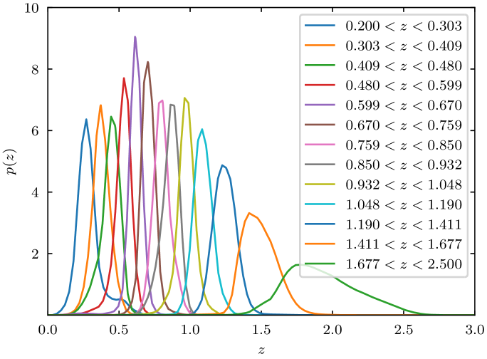
where is the normalized distribution of photometric redshifts shown in Fig. 1. We checked that using the median redshift of each redshift bin did not affect the constraints on , , and (shift smaller than ).
We use Gaussian priors from Planck (Ade et al. 2016) adapted to match the Flagship simulation cosmological parameters so that the ratios between the uncertainties and fiducial values stay the same, yielding and with .
4 Data
4.1 Euclid Flagship simulation
We use the Flagship v.2.1.10 galaxy mock sample (Euclid Collaboration: Castander et al. 2024) available to the Euclid Consortium on CosmoHub 333https://cosmohub.pic.es/ (Tallada et al. 2020; Carretero et al. 2017) created from the Flagship N-body dark matter simulation (Potter et al. 2017). This simulation assumes the following flat CDM cosmology: matter density parameter , baryon density parameter , dark energy density parameter , with a radiation density parameter and for massive neutrinos, dark energy equation of state parameter , reduced Hubble constant , spectral index of the primordial power spectrum , and its amplitude at . This simulation considers a -side box with particles of mass . The main output of the simulation is a lightcone that spans redshifts between and . Dark matter haloes are identified down to with ROCKSTAR (Behroozi et al. 2013). These haloes are then populated with galaxies with halo abundance matching and halo occupation distribution techniques following Carretero et al. (2015). Galaxy luminosities have been calibrated with a combination of the luminosity functions from Blanton et al. (2003), Blanton et al. (2005a), and Dahlen et al. (2005). Galaxy clustering measurements have been calibrated as a function of colour and luminosity following Zehavi et al. (2011) and the colour-magnitude diagram from Blanton et al. (2005b) has been used as a reference.
We apply a magnitude cut at in the VIS band with the additional constraint that only objects with properly determined photometric redshifts are considered (phz_flags = 0). This sample covers one octant of the sky between right ascension and declination for a total area of . Following Euclid Collaboration: Mellier et al. (2024), we divide the sample into 13 equipopulated redshift bins of . The normalized redshift distributions of the 13 bins are shown in Fig. 1. This division yields a large statistic sample, with about million galaxies per redshift bin. Photometric redshifts are defined as the first mode of the probability density functions (PDF) obtained with the k-nearest neighbours algorithm NNPZ (Tanaka et al. 2018) by matching galaxy magnitude and colours to a reference sample of 2 million galaxies simulated up to the depth of the Euclid calibration field and whose PDF are obtained using the template-fitting code Phosphoros (Tucci et al., in prep). The photometric redshift PDF of each galaxy is computed as a weighted average of the PDF of the neighbours found by NNPZ, the weight being the inverse of the distance between the galaxy and the neighbour in the magnitude and colour space. The constraint phz_flags = 0 ensures that the galaxy had enough neighbours found to properly derive the photometric redshift when NNPZ was applied. The photometry used to infer these redshifts has the quality expected from the ground-based observations of the Legacy Survey of Space and Time (LSST, Ivezić et al. 2019) for all galaxies which is optimistic.
The fiducial cosmology used in this paper is a flat CDM cosmology, defined by a set of parameters which match the fiducial cosmology of the Flagship simulation.
5 Results
5.1 Joint BAO measurement
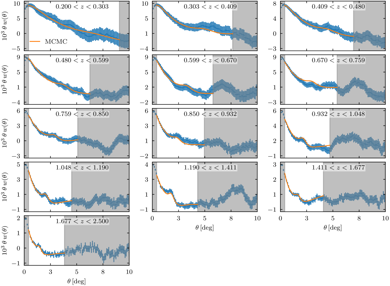
In this section, we present the constraints on obtained with a joint analysis of the 13 redshift bins. We used the template as defined in Sect. 3.2 extended to have bin-specific nuisance parameters , , , and with . Scale cuts are , , visible as grey bands in Fig. 2 and discussed in detail in Sect. 5.6. We clearly see that the position of the BAO peak is found at lower angles as redshift increases, varying from in the first redshift bin to in the last one. We will study the impact of a different choice of scale cuts in Sect. 5.6. We use the analytical covariance (Gaussian and SSC) for this joint analysis.
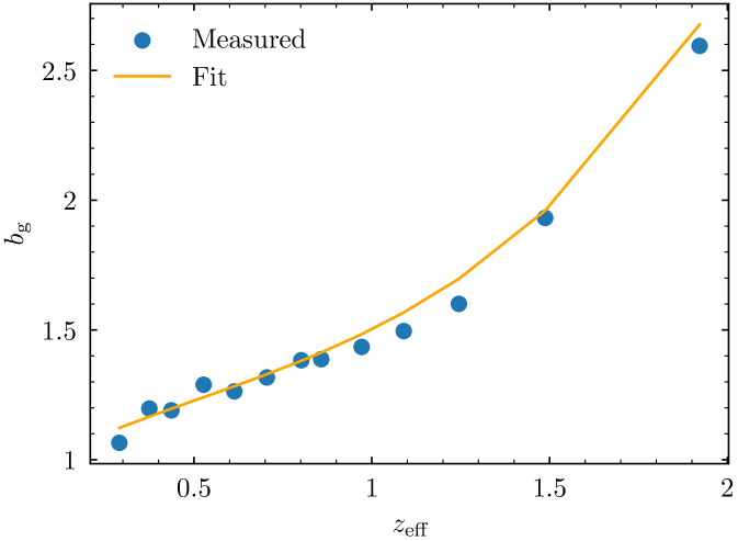
We first report the estimate of the linear galaxy bias, shown in Fig. 3 with the best fit obtained for , , , and as the coefficients of Eq. (18). These values of the bias coefficients are then used to compute the fiducial that will be injected in the template of Eq. (19). Eventual non-linearities of the galaxy bias at small scales or systematic effects are absorbed by the template nuisance parameters without affecting , our parameter of interest.
For this joint analysis with all redshift bins, we report a constraint of , obtained with a profile likelihood approach (Ade et al. 2014). This approach consists in minimizing the while fixing a parameter at various values to obtain a profile of as a function of this parameter. Repeating this with another model of , we can then obtain the difference of the profiles . This result might seem optimistic given that it represents an improvement by a factor of 3 with respect to the latest results from the DES Y6 analysis which yield a constraint of at the 2.4% level with the angular two-point correlation function. However, several factors need to be taken into account in this comparison. The first one is that this work uses data from a simulation and so it is inherently optimistic since it is free from systematic effects while DES Y6 uses real observations and has to correct them. In DES Y6, 5 redshift bins between are used whereas the Flagship sample is here divided into 13 redshift bins between , which increases significantly the constraining power of the joint analysis. We define the significance of the BAO detection to be
| (22) |
evaluated at the value minimizing . The is computed using the transfer function from Eisenstein & Hu (1998) in which the BAO wiggles have been removed, unlike the transfer function from CAMB (Lewis et al. 2000) used to obtain . We quantified with a profile likelihood approach with our data compared to in DES Y6. We also find significantly tighter constraints in each individual redshift bin, contributing to this result.
For this joint analysis, we find that the results obtained with profile likelihood and MCMC differ significantly because of the combined effect of the strong constraining power and the disagreement between the preferred values of in different redshift bins. This leads to a poor exploration of a multi-modal posterior. In more detail, the analytical covariance yields with the MCMC analysis, while considering only the diagonal of the analytical covariance results in . As a comparison, when we only consider the diagonal of the jackknife covariance, we find , which corresponds to a 27% increase of the uncertainty explained by the larger amplitude of the jackknife errors. The results that we obtain from a profile likelihood approach with or without the off-diagonal terms of the analytical covariance are instead similar, with a uncertainty of and , respectively.
We further investigate this result by using a similar approach to DES Y6 by excluding redshift bins in which the BAO signal is not detected with sufficient strength. In this case, is computed for each individual redshift bin and a non-detection is then defined as a detection level . A non-detection in the first bin () is why 5 bins were used in the analysis of DES Y6 instead of 6. After excluding the redshift bins with no significant detection (bins 1, 4, and 6), we report a value , almost identical to the result obtained when including all the redshift bins. The fact that the increase of the uncertainty is as small as 4.5% despite removing three out of 13 bins can be understood by the fact that if redshift bins have no significant detection of the BAO signal then they provide very little constraining power on . We check the robustness of our result with respect to all the redshift bins included in the joint analysis in Sect. 5.2.
An important caveat to fitting a unique to all redshift bins is that it assumes a perfect match between the fiducial cosmology and the true cosmology of the Universe which is unknown. Any mismatch will lead to a variation of which depends on redshift. This effect can be quantified thanks to the definition of in Eq. (20) in which and are computed for different cosmologies while and are constant at the fiducial cosmology of the Flagship simulation. We check that varying , , and by 5% leads to a maximum expected variation of of 1% between the first and last redshift bin. This maximum variation of scales linearly as . Given the constraint obtained on , this effect is non-negligible and is a limit to this joint analysis. For this reason, the analysis is also performed in individual redshift bins in Sect. 5.3.
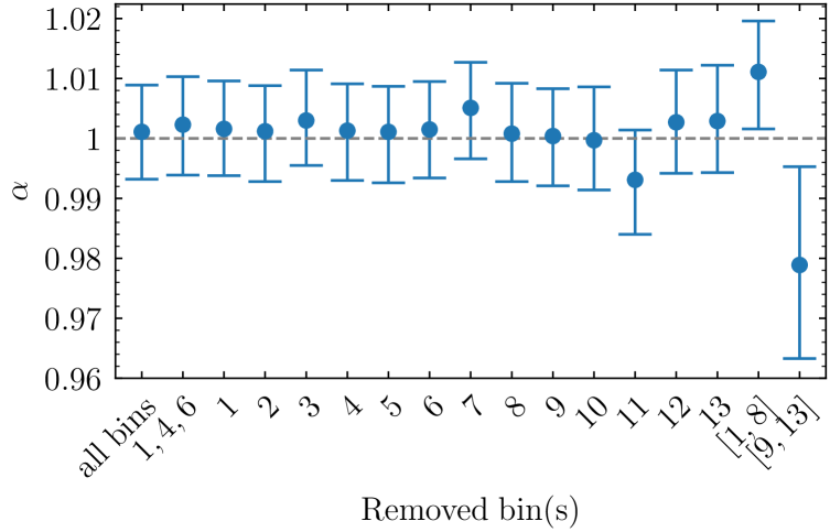
5.2 Robustness validation
In this section, the impact of the different redshift bins in the joint analysis is evaluated by removing each of the 13 redshift bins, one at a time. The constraints on for all these cases are shown in Fig. 4. While most bins have very little effect over the constraints, removing the redshift bin 11 at from the joint analysis decreases by . It also increases uncertainties by 11%, which is expected given that we remove one of the redshift bin with the most constraining power. This constraining power can be understood by studying the properties of the photometric redshifts computed for the Flagship galaxy mock catalogue. Indeed, comparing them to the true redshifts of the simulation using the same binning, we find that with a measure of the scatter robust to outliers and defined as
| (23) |
where , bin 11 has a scatter which is about 25% smaller than bins 12 and 13. The combination of good photometric redshifts and high redshift explains the importance of this bin.
If we compare constraints from bins with redshift to the baseline with all bins, we find that is shifted by towards smaller values and its uncertainty is increased by a factor of two. On the contrary, including high-redshift bins and removing low-redshift bins, the shift towards a larger value of is limited to . The uncertainty is only increased by 14.6%, in this case. These results can be understood in light of the constraints from individual bins detailed in Table 2. Bins at with the largest level of significance of BAO detection are biased towards low values of , which explains why the joint value of increases when they are removed. On the other hand, bins at are overall biased towards larger values of , which explains why removing them decreases the value of the joint . The large difference in the uncertainty values for these last two cases ( against ), can be explained by the much tighter constraints obtained at high redshift, where the BAO peak is not smeared.
5.3 Individual bins BAO measurement
The template fit is now applied to one redshift bin at a time, yielding 13 values of the parameter. This reduces the constraining power over each but gives information about the redshift evolution which can be used to constrain cosmological parameters as explained in Sect. 3.3. It is also a more relevant analysis in our setup given the caveat of fitting a unique explained at the end of Sect. 5.1.
Table 2 groups the results for in all 13 redshift bins, along with the associated sigma level of BAO detection. We first notice that the uncertainty is larger at low redshift. This is due to the smearing of the BAO signal by the non-linear evolution of the large-scale structures under the effect of gravitation. This is clearly visible in Fig. 2 where the BAO is much more peaked at higher redshift. The parameter is compatible with within in all redshift bins with the exception of bin 11 at for which we find a shift. This bin is also the one with the strongest constraining power, explained by the high redshift and small scatter of photometric redshifts . As for the level of detection of the BAO signal, we find three redshift bins with no significant detection, bins 1, 4, and 6. Otherwise, the significance of the detections ranges between 1.1 and detections, with a maximum at and the uncertainty on decreases as the detection level increases, as expected.
| Bin | () | ||
| 1 | 0.290 | no detection | |
| 2 | 0.374 | 1.2 | |
| 3 | 0.436 | 1.1 | |
| 4 | 0.527 | no detection | |
| 5 | 0.613 | 1.1 | |
| 6 | 0.705 | no detection | |
| 7 | 0.802 | 1.5 | |
| 8 | 0.858 | 1.7 | |
| 9 | 0.972 | 1.5 | |
| 10 | 1.090 | 2.7 | |
| 11 | 1.245 | 4.0 | |
| 12 | 1.488 | 2.4 | |
| 13 | 1.922 | 2.9 |
When averaged over all redshift bins, the shift between the results obtained with the jackknife and with the analytical covariances is smaller than with the measured data vector and with a noise-free synthetic data vector computed like the theoretical model.
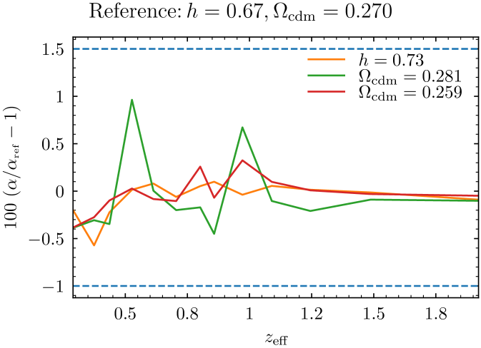
The impact of the choice of fiducial cosmology is investigated by varying from 0.67 to 0.73. Galaxy bias is fitted again before repeating the MCMC analysis bin by bin. We expect a shift of by a factor
| (24) |
After correction by this shift, we measure a remaining maximum relative difference of 0.01, the average over all redshift bins being 0.0012. This is illustrated in Fig. 5. As an additional test, we vary by , keeping and . With and , we respectively find a remaining maximum relative difference of 0.9% and 0.4%, the average over all redshift bins being 0.31% and 0.13%. These variations are negligible compared to the uncertainties on , which shows that the analysis is robust against the choice of fiducial cosmology.
We also provide constraints in a DR1-like setting with a sample divided into 6 redshift bins, a selection cut at , and covering 2500 deg2. The measurement of and BAO analysis were done following the same procedure. In this case, we find that the constraints on in bins 1 to 6 are listed in Table 3.
| Bin | |||||
| 1 | 0.200 | 0.307 | 0.396 | no detection | |
| 2 | 0.396 | 0.432 | 0.507 | no detection | |
| 3 | 0.507 | 0.578 | 0.657 | 1.2 | |
| 4 | 0.657 | 0.727 | 0.840 | 1.2 | |
| 5 | 0.840 | 0.893 | 1.040 | no detection | |
| 6 | 1.040 | 1.325 | 2.500 | 1.1 |
These constraints are in agreement with within . If we compare bins of similar effective redshifts, the constraints are about 20% weaker than with 13 bins in the first bins and significantly worse in the last two bins. The detection of the BAO signal is overall weaker than with 13 redshift bins, with no significant detection in bins 1, 2, and 5 and with in the other bins. These results are expected from the larger uncertainties on and the larger bins : intra-bin variations of the BAO scale dilute the signal. Note that the LSST-like photometry assumed to infer photometric redshifts is even more optimistic for this setting than for the previous one, since this photometry will not be available at the time of this data release. Instead, photometry from the Dark Energy Survey will be used (Abbott et al. 2018). For this reason, the fact that the redshift distribution is well known is only true with the Flagship simulation. With data, calibrating the bias and stretch prior to the analysis will be mandatory, as in Abbott et al. (2024). Ideally, these nuisance parameters for the bias and stretch of will be marginalized over in the MCMC analysis of DR1 data as in Bertmann et al., in prep. These constraints could probably be improved with analysis choices tailored to this sample, for example with different scale cuts.
5.4 Cosmological constraints from BAO
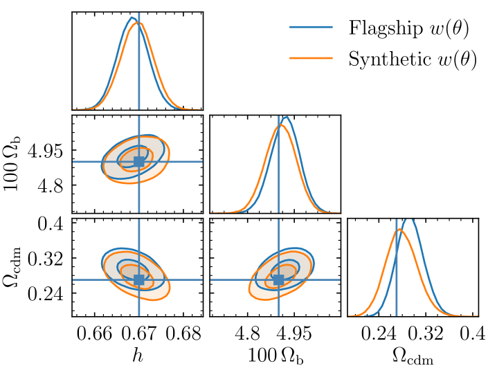
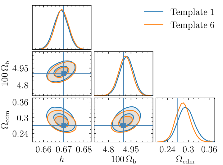
One can constrain the , , and parameters by sampling them in their dependence with respect to the values of , (Eq. (20) and Appendix A) obtained by template fitting in each individual bin. We list in Table 2 the values of and the associated uncertainties obtained by MCMC analysis. In Fig. 6, we show the constraints on , , and . We obtain , , and , which is in agreement with the simulation cosmology. Using the synthetic data vector instead of the measured two-point angular correlation function to extract the and then obtain cosmological constraints with the same analysis, we check that the bias on decreases from to .
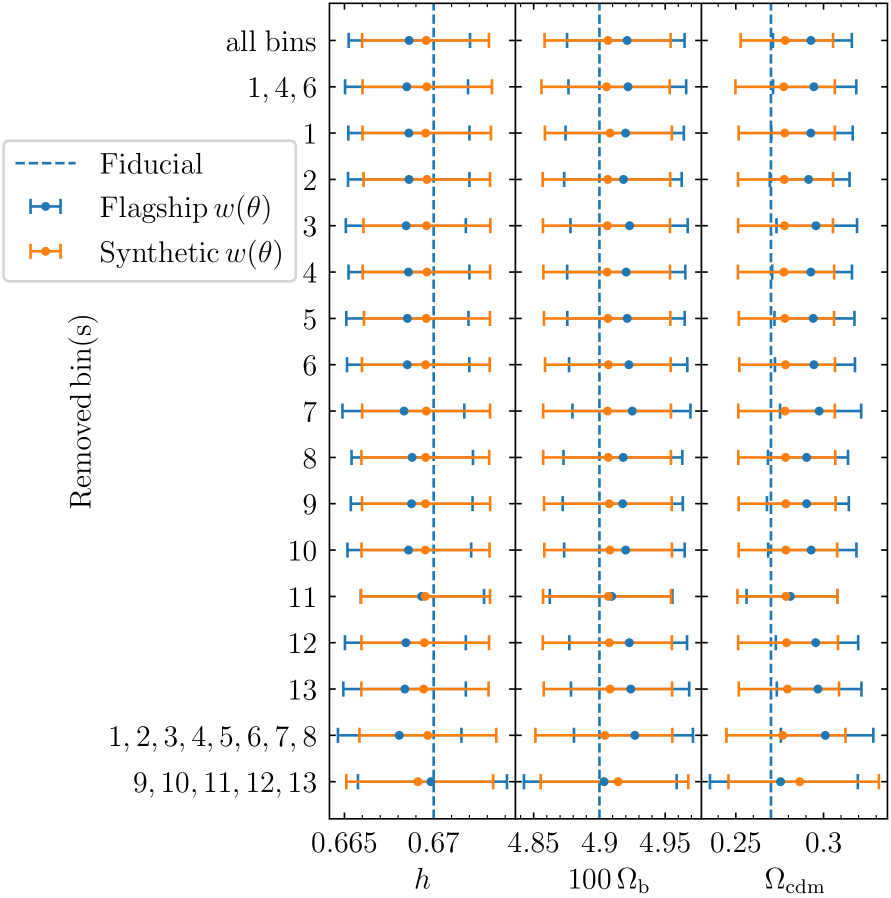
We check how excluding one or some redshift bins from this analysis affects the cosmological constraints. Figure 7 groups all results for , , and with Planck priors. We consider the , obtained by template fitting on measured on Flagship in blue, or a noise-free synthetic computed like the theoretical model in orange. We first remove one redshift bin at a time. With the measured , redshift bin 11 seems to have a large weight in shifting towards smaller values: when it is excluded, we recover a less biased estimate of , , and with a shift of 0.3, 0.2, and respectively. Removing the other bins has a much smaller effect. Results are also shown when removing redshift bins with no BAO detection (bins 1, 4, and 6), low-redshift bins (1 to 8), and high-redshift bins (9 to 13). Apart from the effect seen from removing bin 11, we find that high-redshift bins tend to bias towards lower values while and are biased towards larger values. However, high-redshift bins also provide the tightest constraints, with an increase of the uncertainty of , , and by 23%, 30%, and 87% respectively when they are removed. Replacing obtained from the measured by the ones from a synthetic , we find that shifts of , , and (shown in orange in Fig. 7) with respect to their fiducial values are on average decreasing from 0.4, 0.4, and to 0.1, 0.1, and . The constraining power is also robust with respect to the choice of bins when excluded one by one, with an average variation smaller than 2% for and , and 7% for . With the synthetic data vector, the increase of the uncertainties when removing high redshifts is smaller with 16%, 17%, and 63% against 23%, 30%, and 87% with the measured .
5.5 Comparison of fitting templates
The polynomial correction applied in the template is defined arbitrarily and different choices can be found in the literature. It is important to check whether the polynomial includes enough orders to absorb eventual non-linearities of the galaxy bias. In this context, we explore ten different combinations of orders leading to ten templates using the same scale cuts and fiducial cosmology as for the analysis of the individual bins. The templates considered in this analysis are
-
•
template 1: ,
-
•
template 2: ,
-
•
template 3: ,
-
•
template 4: ,
-
•
template 5: ,
-
•
template 6: ,
-
•
template 7: ,
-
•
template 8: ,
-
•
template 9: ,
-
•
template 10: .
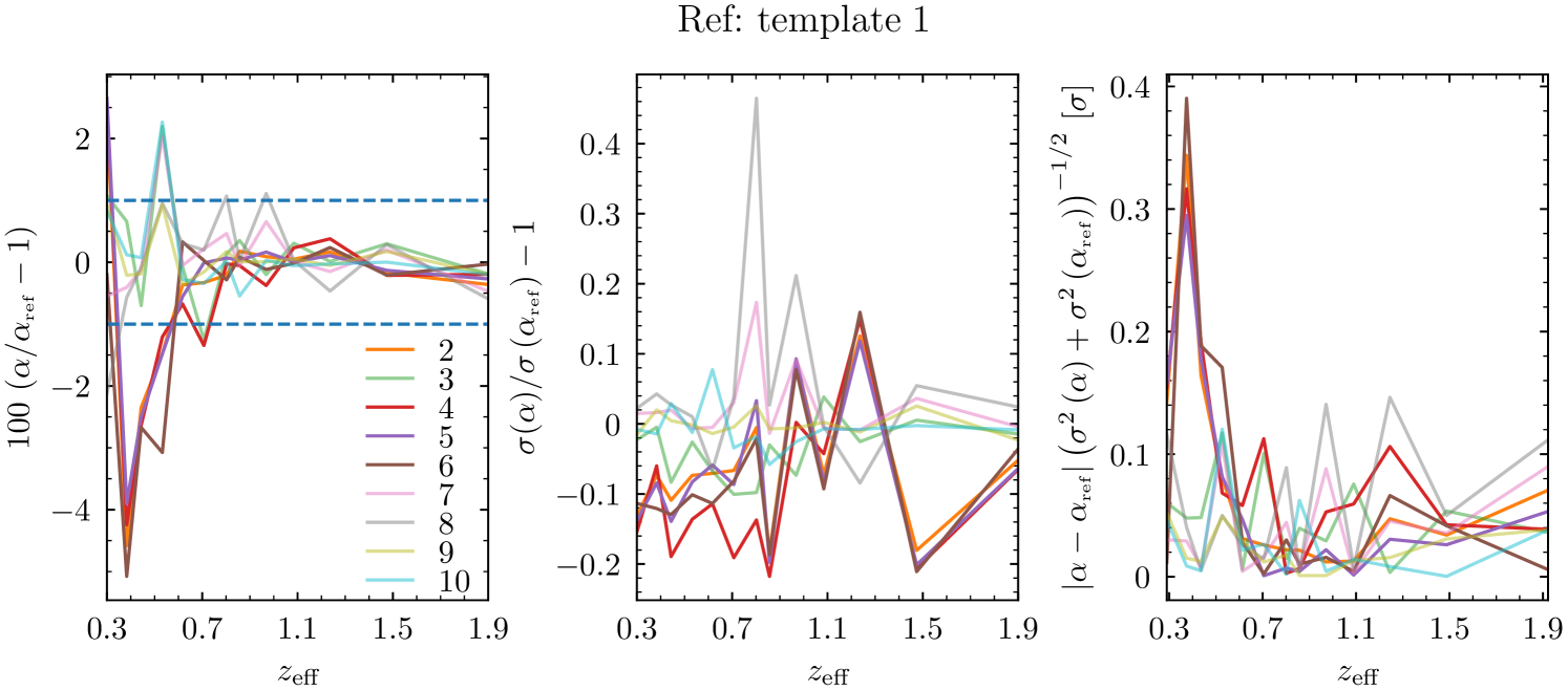
The comparison of the resulting for each template with respect to the fiducial template 1 is shown in Fig. 8. Constraints from templates 2, 4, 5, and 6 are highlighted because they are consistent with each other and quite different from the reference at low redshift. These templates do not have a term in . From this observation, it seems that this order is needed. We find that the uncertainty on is systematically underestimated by 10% with templates 2, 4, 5, and 6. This result is still observed when a noise-free synthetic data vector is used instead of the measured two-point correlation function. On the contrary, we see almost no variation of the results between the other templates with additional orders . The agreement of the various measurements of with these templates defined as remains within . This trend is also observed when cosmological constraints are inferred, with a small but very clear shift in the posterior distributions of for templates 2, 4, 5, and 6, as shown in Fig. 9. Given the similar constraints between the other templates, template 1 was chosen for the main analysis.
Another important aspect of the robustness of the template is to be able to handle shifts of the fiducial cosmology with respect to the true cosmology. As such, the previous comparison has been repeated in a setup where the fiducial cosmology was altered to differ from the cosmology from the Flagship simulation, using instead of . In this case, we find that the absolute shift of with respect to the expected value of 1 averaged over all redshift bins for templates 1, 3, 7, 8, 9, 10 (we exclude templates without order ) is respectively 0.030, 0.033, 0.030, 0.030, 0.031, and 0.032. Table 4 presents the results of this test, showing no preference for including higher orders in the template polynomial when it comes to robustness with respect to the choice of fiducial cosmology.
| Template | Bin 1 | Bin 2 | Bin 3 | Bin 4 | Bin 5 | Bin 6 | Bin 7 | Bin 8 | Bin 9 | Bin 10 | Bin 11 | Bin 12 | Bin 13 | ||
| 1 | 1.013 | 1.046 | 0.969 | 1.011 | 1.012 | 0.996 | 0.949 | 1.069 | 1.047 | 1.032 | 1.049 | 1.011 | 1.010 | 0.030 | 0.068 |
| 3 | 1.038 | 1.057 | 0.956 | 1.014 | 1.003 | 0.979 | 0.949 | 1.066 | 1.038 | 1.033 | 1.048 | 1.012 | 1.009 | 0.033 | 0.064 |
| 7 | 1.010 | 1.042 | 0.970 | 1.027 | 1.010 | 0.996 | 0.952 | 1.068 | 1.056 | 1.032 | 1.047 | 1.013 | 1.007 | 0.030 | 0.070 |
| 8 | 0.992 | 1.052 | 0.969 | 1.017 | 1.015 | 1.000 | 0.956 | 1.070 | 1.059 | 1.032 | 1.045 | 1.015 | 1.005 | 0.030 | 0.070 |
| 9 | 1.034 | 1.052 | 0.970 | 1.016 | 1.005 | 0.994 | 0.949 | 1.067 | 1.049 | 1.032 | 1.048 | 1.012 | 1.009 | 0.031 | 0.067 |
| 10 | 1.026 | 1.052 | 0.967 | 1.016 | 1.012 | 0.993 | 0.947 | 1.063 | 1.048 | 1.032 | 1.048 | 1.012 | 1.010 | 0.032 | 0.062 |
5.6 Effect of the scale cuts
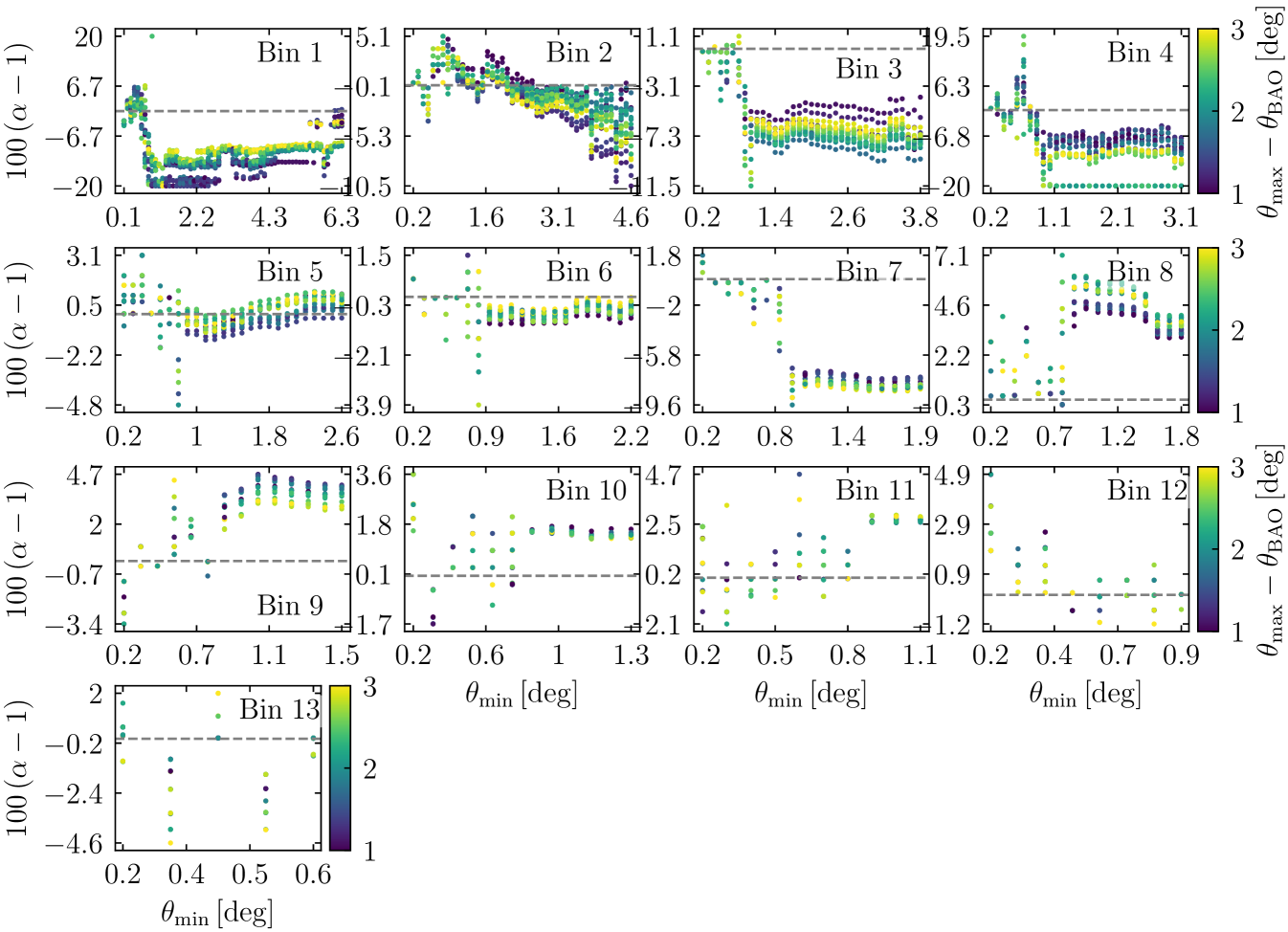
The large redshift range included in this configuration space analysis entails that varies between and . In this situation, using a single scale cut for all bins or a redshift-dependent one is not obvious. We performed a first study of how varies as a function of and with a fitting approach on a grid defined by and by steps of . The smallest data vector considered is with 20 points.
The results of this study are shown in Fig. 10. The bias varies with , with a clear cut-off at . Increasing beyond this cut-off tends to bias , especially at low redshift, where the BAO signal is smeared by the non-linear evolution of large-scale structures. While a pronounced evolution of with is visible at low redshift when , no clear trend can be found when , where the bias is the smallest.
Following these observations, we then carried out an MCMC study on a smaller grid defined as with the same resolution and with steps of . On this grid, no significant variation of was observed with both and . The same observations were made when the analytical Gaussian covariance was used instead of the jackknife covariance. The final scale cut chosen was then as it yielded the most robust results across all redshift bins. In the grid used for the MCMC, the extracted in all bins are in agreement within on average and at most . The effect on , , and inferred from the is on average and never exceeds .
5.7 Impact of RSD
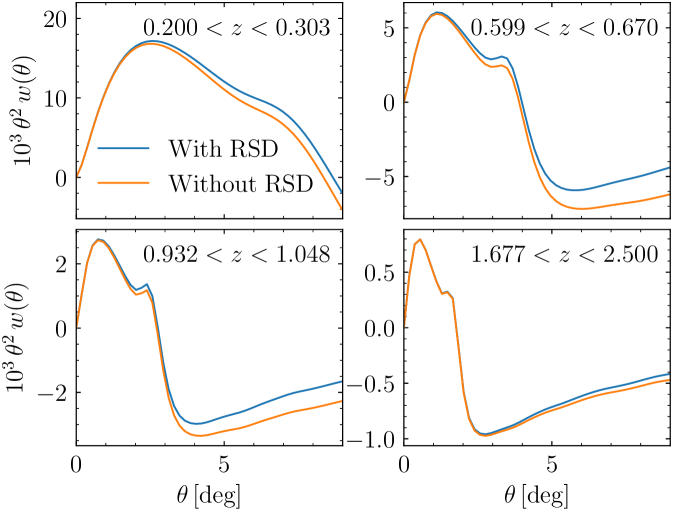
In this section, we check whether including RSD in the theoretical model described in Sect. 2.1 affects the constraints on . The effect of RSD over the two-point angular correlation function is illustrated in Fig. 11. The correlation function amplitude is increased at large scales and low redshift. This is the Kaiser effect, explained by the inflow of galaxies towards overdensities, which is stronger at low redshift (Kaiser 1987).
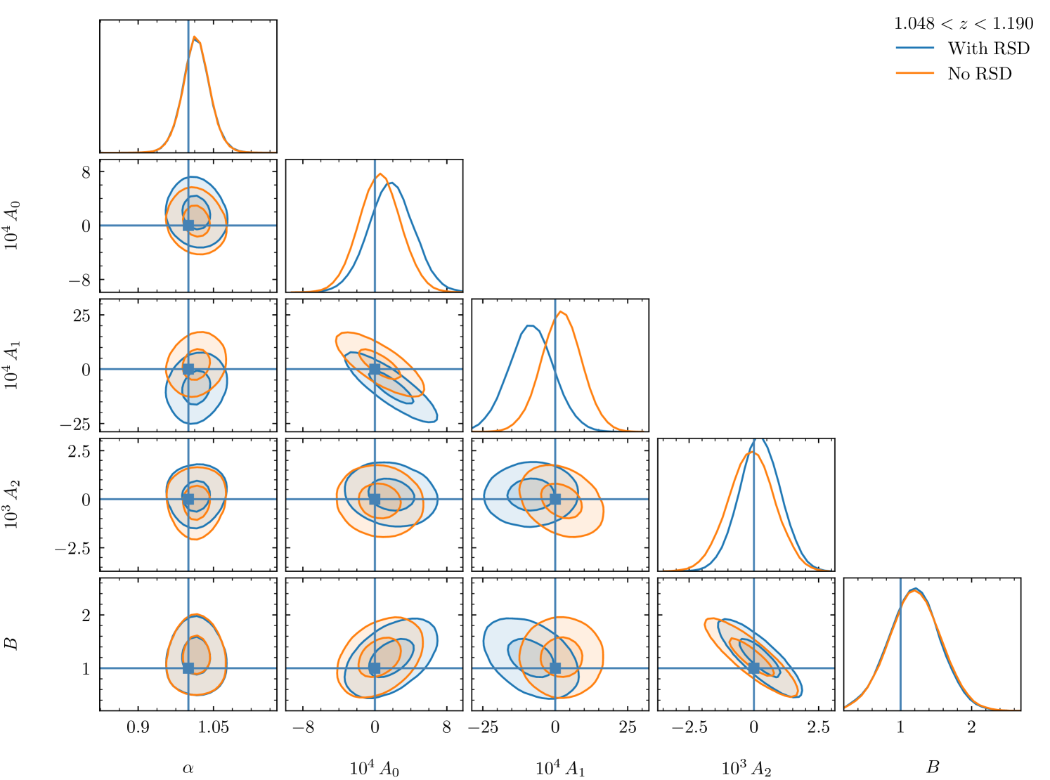
However, the actual position of the BAO scale remains unchanged and we see in Fig. 12 that this is reflected in the constraints obtained from MCMC analysis. When RSD are included, in blue in the figure, the template nuisance parameters compensate for the effect of RSD with a significant decrease of , while and are slightly increased. This trend holds in all redshift bins except the last one where the amplitude of the shifts becomes negligible. The relative difference averaged over all redshift bins is 0.25%, the maximum being 0.5%. As for the uncertainty of , its variations do not exceed 3.7% and are on average 1.4%. Thanks to the template-fitting approach, the analysis is robust with respect to RSD. In any case, as explained in Sect. 2.1, RSD are included in the analysis.
5.8 Effect of the redshift binning scheme
In this section, we show the effect of the choice of using equidistant redshift bins compared to the constraints obtained with equipopulated bins while keeping the same fiducial choice of template and scale cuts. This choice results in bins of width . For this analysis, the two-point correlation function and galaxy bias are measured in the same way as described in Sect. 2.2 for the equipopulated binning scheme. The rest of the analysis is carried out in an identical way. Using this binning scheme, we get equivalent constraints for redshift bins of similar , as reported in Table 5. Note that the equidistant binning does not entail regularly spaced . The effective redshifts are still computed with Eq. (21). By construction, we have more bins with high where the BAO signal is not smeared by the non-linear evolution of structures due to gravitation. Simultaneously, thinner redshift bins present a BAO signal which is less diluted by intra-bin variations of the BAO scale. However, the decrease in number density entails that the error bars of the two-point correlation function are larger at high redshift. In our case, this compromise yields more bins with high detection levels and tight constraints on . We also find several bins with low values of , two of them being more than away from , at and 2.174.
| Bin | () | ||
| 1 | 0.311 | no detection | |
| 2 | 0.442 | 1.0 | |
| 3 | 0.63 | no detection | |
| 4 | 0.806 | 1.2 | |
| 5 | 0.961 | 1.3 | |
| 6 | 1.126 | 2.0 | |
| 7 | 1.286 | 4.1 | |
| 8 | 1.474 | 2.5 | |
| 9 | 1.641 | 2.2 | |
| 10 | 1.82 | 3.4 | |
| 11 | 1.993 | 3.3 | |
| 12 | 2.174 | 2.0 | |
| 13 | 2.365 | 4.6 |
Propagating these results to the cosmological parameters, we find , , and , which represents shifts of +0.1%, 0.5%, and +9.2% respectively, and a 36.4% improvement in the constraining power for with respect to the equipopulated binning results. The variations in the parameter values are driven by the low value and tight constraints of bin 11 in the equidistant binning. Bin 12 has an even lower value and participates to these variations but in a weaker way due to its uncertainty, larger than in bin 11 by a factor 2.1. Given these results, it seems that the equidistant scheme may be more suitable for the BAO analysis than the equipopulated scheme initially chosen to match the choice that maximizes the dark energy figure of merit of the 32-point analysis for Euclid. In future Euclid BAO photometric analyses, an optimization of the photometric sample selection will by necessary.
6 Conclusions
In this work, we have estimated our ability to constrain cosmological parameters with the photometric sample of Euclid through a BAO analysis of the Flagship mock galaxy catalogue, whose area is intermediate to the expected observed survey area at Data Release 1 and 2. We have measured the two-point correlation function in 13 redshift bins. We have extracted constraints on the BAO signal through the parameter in each redshift bin but also using all bins jointly. The significance of the BAO detection has been quantified to reach with the joint analysis, a three-fold improvement with respect to the latest results in photometric surveys (DES Y6), with similar or better constraints in all redshift bins, covering also a large range of redshifts . This result shows how powerful photometric galaxy clustering can be with Euclid. From these BAO constraints and considering Planck priors, we have derived constraints on different cosmological parameters: , , and in a flat CDM cosmology.
We have also studied different analysis choices, showing that scale cuts can have a non-negligible effect over the value of the parameter. Indeed, if , then we observe a bias, even for low-redshift bins where the BAO peak is at large scales. On the contrary, while omitting the order in the template biases the resulting cosmological constraints, there is no need to include higher orders in the template functional form used to fit the BAO feature. The template is robust to the choice of fiducial cosmology, with variations not exceeding 0.0031 when averaged over all redshifts, well below the uncertainties of given in Table 2. The template is efficient when it comes to absorbing effects that affect the amplitude of the two-point angular correlation function like RSD: including or removing them from the model, the constraints over remain unchanged at all redshifts. An important point which has been seen in both joint and individual redshift bin analyses is the robustness with respect to the redshift bins included in the analysis. We have also checked that there is no significant bias when a synthetic data vector is used. However, when we consider the data vector measured on the Flagship simulation, we have observed a shift of the parameter and an increase of its uncertainty when redshift bin 11 is excluded. This effect is seen in both the joint analysis and the cosmological parameters inferred from , . This is explained by the fact that this bin has the largest BAO detection significance. This detailed study of the effect of each redshift bin will be mandatory in future works, given that the strength of the BAO signal and its effect over cosmological constraints change with redshift.
Results from Sect. 5.8 suggest that there is margin for improvement in the constraints obtained from a BAO analysis by optimising the redshift binning scheme. A galaxy sample selection taking into account both redshift and colour could be another possible point of improvement for these results. However, it is very promising to see that with a simulated area of 37% of what is expected at Data Release 3 of Euclid, the constraints on are already improved by a factor three with respect to the current best constraints from a single photometric survey.
Acknowledgements.
The Euclid Consortium acknowledges the European Space Agency and a number of agencies and institutes that have supported the development of Euclid, in particular the Agenzia Spaziale Italiana, the Austrian Forschungsförderungsgesellschaft funded through BMK, the Belgian Science Policy, the Canadian Euclid Consortium, the Deutsches Zentrum für Luft- und Raumfahrt, the DTU Space and the Niels Bohr Institute in Denmark, the French Centre National d’Etudes Spatiales, the Fundação para a Ciência e a Tecnologia, the Hungarian Academy of Sciences, the Ministerio de Ciencia, Innovación y Universidades, the National Aeronautics and Space Administration, the National Astronomical Observatory of Japan, the Netherlandse Onderzoekschool Voor Astronomie, the Norwegian Space Agency, the Research Council of Finland, the Romanian Space Agency, the State Secretariat for Education, Research, and Innovation (SERI) at the Swiss Space Office (SSO), and the United Kingdom Space Agency. A complete and detailed list is available on the Euclid web site (www.euclid-ec.org). This work has made use of CosmoHub, developed by PIC (maintained by IFAE and CIEMAT) in collaboration with ICE-CSIC. It received funding from the Spanish government (MCIN/AEI/10.13039/501100011033), the EU NextGeneration/PRTR (PRTR-C17.I1), and the Generalitat de Catalunya. Some of the results in this paper have been derived using the healpy and HEALPix packages. SC acknowledges support from the Italian Ministry of University and Research (mur), PRIN 2022 ‘EXSKALIBUR – Euclid-Cross-SKA: Likelihood Inference Building for Universe’s Research’, Grant No. 20222BBYB9, CUP C53D2300131 0006, and from the European Union – Next Generation EU.References
- Abbott et al. (2018) Abbott, T. M. C., Abdalla, F. B., Allam, S., et al. 2018, ApJS, 239, 18
- Abbott et al. (2024) Abbott, T. M. C., Adamow, M., Aguena, M., et al. 2024, Phys. Rev. D, 110, 063515
- Ade et al. (2016) Ade, P. A. R., Aghanim, N., Arnaud, M., et al. 2016, A&A, 594, A13
- Ade et al. (2014) Ade, P. A. R., Aghanim, N., Arnaud, M., et al. 2014, A&A, 566, A54
- Alonso et al. (2015) Alonso, D., Bull, P., Ferreira, P. G., Maartens, R., & Santos, M. G. 2015, ApJ, 814, 145
- Behroozi et al. (2013) Behroozi, P. S., Wechsler, R. H., & Wu, H.-Y. 2013, ApJ, 762, 109
- Blanton et al. (2003) Blanton, M. R., Hogg, D. W., Bahcall, N. A., et al. 2003, ApJ, 592, 819
- Blanton et al. (2005a) Blanton, M. R., Lupton, R. H., Schlegel, D. J., et al. 2005a, ApJ, 631, 208
- Blanton et al. (2005b) Blanton, M. R., Schlegel, D. J., Strauss, M. A., et al. 2005b, AJ, 129, 2562
- Blas et al. (2011) Blas, D., Lesgourgues, J., & Tram, T. 2011, JCAP, 07, 034
- Carretero et al. (2015) Carretero, J., Castander, F. J., Gaztañaga, E., Crocce, M., & Fosalba, P. 2015, MNRAS, 447, 646
- Carretero et al. (2017) Carretero, J., Tallada, P., Casals, J., et al. 2017, in Proceedings of the European Physical Society Conference on High Energy Physics. 5-12 July, 488
- Challinor & Lewis (2011) Challinor, A. & Lewis, A. 2011, Phys. Rev. D, 84, 043516
- Chisari et al. (2019) Chisari, N. E., Alonso, D., Krause, E., et al. 2019, ApJS, 242, 2
- Cole et al. (2005) Cole, S., Percival, W. J., Peacock, J. A., et al. 2005, MNRAS, 362, 505
- Crocce et al. (2011) Crocce, M., Cabré, A., & Gaztañaga, E. 2011, MNRAS, 414, 329
- Dahlen et al. (2005) Dahlen, T., Mobasher, B., Somerville, R. S., et al. 2005, ApJ, 631, 126
- Dembinski et al. (2020) Dembinski, H., Ongmongkolkul, P., Deil, C., et al. 2020, Zenodo, 10.5281/zenodo.3949207
- DESI Collaboration: Adame et al. (2024) DESI Collaboration: Adame, A., Aguilar, J., Ahlen, S., et al. 2024, arXiv e-prints, arXiv:2404.03000
- Eisenstein & Hu (1998) Eisenstein, D. J. & Hu, W. 1998, ApJ, 496, 605
- Eisenstein et al. (2005) Eisenstein, D. J., Zehavi, I., Hogg, D. W., et al. 2005, ApJ, 633, 560
- Euclid Collaboration : Sciotti et al. (2024) Euclid Collaboration : Sciotti, D., Gouyou Beauchamps, S., Cardone, V. F., et al. 2024, A&A, 691, A318
- Euclid Collaboration: Blanchard et al. (2020) Euclid Collaboration: Blanchard, A., Camera, S., Carbone, C., et al. 2020, A&A, 642, A191
- Euclid Collaboration: Castander et al. (2024) Euclid Collaboration: Castander, F. J., Fosalba, P., Stadel, J., et al. 2024, A&A, accepted, arXiv:2405.13495
- Euclid Collaboration: Cropper et al. (2024) Euclid Collaboration: Cropper, M., Al-Bahlawan, A., Amiaux, J., et al. 2024, A&A, accepted, arXiv:2405.13492
- Euclid Collaboration: Jahnke et al. (2024) Euclid Collaboration: Jahnke, K., Gillard, W., Schirmer, M., et al. 2024, A&A, accepted, arXiv:2405.13493
- Euclid Collaboration: Mellier et al. (2024) Euclid Collaboration: Mellier, Y., Abdurro’uf, Acevedo Barroso, J. A., et al. 2024, A&A, accepted, arXiv:2405.13491
- Fang et al. (2020b) Fang, X., Eifler, T., & Krause, E. 2020b, MNRAS, 497, 2699
- Fang et al. (2020a) Fang, X., Krause, E., Eifler, T., & MacCrann, N. 2020a, JCAP, 05, 010
- Foreman-Mackey et al. (2013) Foreman-Mackey, D., Hogg, D. W., Lang, D., & Goodman, J. 2013, PASP, 125, 306
- Gelman & Rubin (1992) Gelman, A. & Rubin, D. B. 1992, Statistical Science, 7, 457
- Górski et al. (2005) Górski, K. M., Hivon, E., Banday, A. J., et al. 2005, ApJ, 622, 759
- Gouyou Beauchamps et al. (2022) Gouyou Beauchamps, S., Lacasa, F., Tutusaus, I., et al. 2022, A&A, 659, A128
- Hartlap et al. (2007) Hartlap, J., Simon, P., & Schneider, P. 2007, A&A, 464, 399
- Hu & Sugiyama (1996) Hu, W. & Sugiyama, N. 1996, ApJ, 471, 542
- Ivezić et al. (2019) Ivezić, Ž., Kahn, S. M., Tyson, J. A., et al. 2019, ApJ, 873, 111
- James & Roos (1975) James, F. & Roos, M. 1975, Comput. Phys. Commun., 10, 343
- Jarvis et al. (2004) Jarvis, M., Bernstein, G., & Jain, B. 2004, MNRAS, 352, 338
- Kaiser (1987) Kaiser, N. 1987, MNRAS, 227, 1
- Kaiser (1992) Kaiser, N. 1992, ApJ, 388, 272
- Krause & Eifler (2017) Krause, E. & Eifler, T. 2017, MNRAS, 470, 2100
- Lacasa & Grain (2019) Lacasa, F. & Grain, J. 2019, A&A, 624, A61
- Landy & Szalay (1993) Landy, S. D. & Szalay, A. S. 1993, ApJ, 412, 64
- Lepori et al. (2022) Lepori, F., Tutusaus, I., Viglione, C., et al. 2022, A&A, 662, A93
- Lewis et al. (2000) Lewis, A., Challinor, A., & Lasenby, A. 2000, ApJ, 538, 473
- Mather et al. (1999) Mather, J. C., Fixsen, D. J., Shafer, R. A., Mosier, C., & Wilkinson, D. T. 1999, ApJ, 512, 511
- Mead et al. (2021) Mead, A. J., Brieden, S., Tröster, T., & Heymans, C. 2021, MNRAS, 502, 1401
- Percival et al. (2001) Percival, W. J., Baugh, C. M., Bland-Hawthorn, J., et al. 2001, MNRAS, 327, 1297
- Potter et al. (2017) Potter, D., Stadel, J., & Teyssier, R. 2017, CompAC, 4, 2
- Tallada et al. (2020) Tallada, P., Carretero, J., Casals, J., et al. 2020, Astronomy and Computing, 32, 100391
- Tanaka et al. (2018) Tanaka, M., Coupon, J., Hsieh, B.-C., et al. 2018, PASJ, 70, S9
- Troxel et al. (2018) Troxel, M. A., Krause, E., Chang, C., et al. 2018, MNRAS, 479, 4998
- Tutusaus et al. (2020) Tutusaus, I., Martinelli, M., Cardone, V. F., et al. 2020, A&A, 643, A70
- Zehavi et al. (2011) Zehavi, I., Zheng, Z., Weinberg, D. H., et al. 2011, ApJ, 736, 59
- Zonca et al. (2019) Zonca, A., Singer, L., Lenz, D., et al. 2019, Journal of Open Source Software, 4, 1298
Appendix A Computation of
In our analysis, we compute following the fast approximations described by Eqs. (2) to (6) in Eisenstein & Hu (1998). In these equations, we updated the CMB temperature to its value reported in the final FIRAS CMB results (Mather et al. 1999). We report here the expressions used for the redshift and wavenumber of the particle horizon at the matter-radiation equality, in which , as well as the expression used for
| (25) | ||||
| (26) | ||||
| (27) | ||||
| (28) | ||||
| (29) |
Then we compute the distance as
| (31) | |||
| (32) | |||
| (33) |
The prefactor 1345 in Eq. (LABEL:eq:z_drag_eisenstein) was taken from Eq. (E-2) in Hu & Sugiyama (1996) rather than the 1291 prefactor used in Eisenstein & Hu (1998) because we find a significantly better agreement with the results from the Boltzmann codes CAMB and CLASS (Blas et al. 2011). Varying , , or in [0.6,0.8], [0.039,0.059], and [0.17,0.37] respectively while fixing the other parameters to the fiducial values of Flagship, we find an average relative difference of , 0.01%, and 0.03% using 1345 as a prefactor against of 2.7%, 2.7%, and 2.6% using 1291.