Euclid Quick Data Release (Q1)
The SPE processing function (PF) of the Euclid pipeline is dedicated to the automatic analysis of one-dimensional spectra to determine redshifts, line fluxes, and spectral classifications. The first Euclid Quick Data Release (Q1) delivers these measurements for all objects identified in the photometric survey. In this paper, we present an overview of the SPE PF algorithm and assess its performance by comparing its results with high-quality spectroscopic redshifts from the Dark Energy Spectroscopic Instrument (DESI) survey in the Euclid Deep Field North. Our findings highlight remarkable accuracy in successful redshift measurements, with a bias of less than in and a high precision of approximately . The majority of spectra have only a single spectral feature or none at all. To avoid spurious detections, where noise features are misinterpreted as lines or lines are misidentified, it is therefore essential to apply well-defined criteria on quantities such as the redshift probability or the flux and signal-to-noise ratio. Using a well-tuned quality selection, we achieve an 89% redshift success rate in the target redshift range for cosmology (), which is well covered by DESI for . Outside this range where the line is observable, redshift measurements are less reliable, except for sources showing specific spectral features (e.g., two bright lines or strong continuum). The classification based on the spectroscopy alone is effective for galaxies (about 80% success rate), while it is currently less efficient for stars and quasars (%). Ongoing refinements along the entire chain of PFs are expected to enhance both the redshift measurements and the spectral classification, allowing us to define the large and reliable sample required for cosmological analyses. Overall, the Q1 SPE results are promising, demonstrating encouraging potential for cosmology.
Key Words.:
Surveys – Cosmology: observations – Methods: data analysis – Techniques: imaging spectroscopy – Galaxies: distances and redshifts1 Introduction
One of the two main objectives of the Euclid mission (Euclid Collaboration: Mellier et al. 2024) is to measure galaxy clustering in the redshift interval (hereafter, the ‘target range’), using spectroscopic redshifts measured on the spectra provided by the Near Infrared Spectro-Photometer (NISP) instrument (Euclid Collaboration: Jahnke et al. 2024). The spectra have a resolution , cover the wavelength range 1206–1892 , and redshifts in the target range are measured by identifying the emission line. NISP is a slitless spectrometer, which means that the spectra of all objects on the sky potentially leave a trace on the spectroscopic exposures. The only condition for a spectrum to be extracted is that a corresponding object is identified in the photometric catalogue constructed from Euclid imaging. This paper presents spectroscopic measurements and redshifts released in the framework of the first ‘Quick Release’ of Euclid products (Euclid Quick Release Q1 2025; Euclid Collaboration: Aussel et al. 2025), for objects brighter than and observed over the area of the Euclid Deep Fields (EDSs) in the configuration of the Euclid Wide Survey (EWS). However, given the specific objectives of the mission, in terms of redshift range and emission-line flux, as well as wavelength domain and intrinsic quality of the spectra, these data cannot be used as a homogeneous set for blind statistical studies, and special attention must be paid to redshift values outside the target range or with lines fainter than the nominal limit of the survey. In addition, we describe the output and performance of the sole spectroscopy channel, while the final analysis of Euclid will benefit from the combination with the high-quality visible and infrared images provided by both the VIS (Euclid Collaboration: Cropper et al. 2024) and NISP instruments.
The paper is organised as follows. Section 2 describes the various spectroscopic products that are present in the Euclid scientific archive, together with the main parameters that are useful in extracting the best measurements, as well as a brief description of the methods of redshift calculation. Section 3 gives results on the efficiency and accuracy of the redshift measurements, while the results of the spectroscopic classification are presented in Sect. 4. Section 5 gives information about the quality and performance of the emission-line fluxes, and Sect. 6 discusses the quality of the redshift measurement for various subsamples with respect to existing redshift catalogues.
2 SPE PF methods and product description
2.1 SPE PF spectra handling and basic description
The Euclid data processing is handled by the Science Ground Segment, which is split into Processing Functions (PFs), each taking care of a specific aspect. The Spectroscopy PF (SPE PF) is in charge of redshift estimation, measurement-reliability calculation, and spectroscopic classification of all objects present in the main catalogue created by the ‘merge’ PF (MER PF, Euclid Collaboration: Romelli et al. 2025). SPE PF first reads the 1D spectra produced by SIR PF (Euclid Collaboration: Copin et al. 2025) by combining the four individual exposures taken with different orientations of the grisms (see Euclid Collaboration: Scaramella et al. 2022 for details on the observing strategy). The data provided by SIR PF also include flags describing the quality of each pixel in the spectrum and the number of individual exposures that actually contributed to its final value. For this Q1 release, only the spectra of objects with were extracted. At fainter magnitudes, the catalogues derived from NISP imaging suffer from significant contamination by fake sources, due to the persistence effect in infrared detectors. Spurious residuals from preceding spectroscopic exposures are detected on the following photometric images, thus preventing SIR PF from reliably extracting source positions at (see Euclid Collaboration: Polenta et al. 2025 for a description of the NIR PF and the persistence phenomenon). Before proceeding with the redshift estimate, pixels that were flagged as “do not use” by SIR PF are discarded (see Euclid Collaboration: Copin et al. 2025 for details on flags). Following tests performed on simulated data and early spectra to eliminate as many artificial features as possible, only pixels that are built from at least three exposures are retained. This is the minimum number to guarantee a proper performance of the PF-SIR sigma-clipping combination.
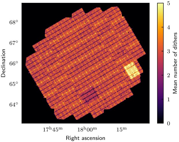
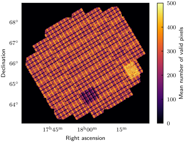
We also discard pixels that have the sixth bit of the quality flag activated: this corresponds to pixels at the edges of the spectrum, for which the absolute flux calibration curve has values close to zero, making calibration uncertain. Because of the current SIR configuration, this flag limits the available redshift interval to 0.9–1.8 in this release. Accounting also for the various edge effects (size of the fields, focal plane geometry, and gaps between detectors – see Fig. 1), yields a sample of 3.8 million processed spectra, among the 5.1 million objects in the catalogue, over the 63.1 deg2 Q1 area. This includes all spectra with at least one valid pixel. To approach a science-grade sample, a lower threshold to the number of valid pixels is clearly required; however, at this stage we chose not to apply any such cut, since future improvements in the pipeline may lead to different values for the optimal selection to be used. The nominal length of a spectrum that would not contain any invalid pixel is about 470 pixels.
It is important to note that this sample of processed (and delivered) spectra is in fact nearly two orders of magnitude larger than the number of emitters whose redshifts are expected to be measurable at the depth of the EWS, within the Q1 area. Following the original science requirements of the mission, the NISP spectrograph was designed as to secure a redshift for an average number of galaxies per deg2, at a flux limit . Because of measuring redshifts using only the line detection (see discussion in the following sections), by construction these galaxies will have a redshift within the target range . In practice, this implies that within the Q1 release we would expect at best to recover a total of redshifts within the target range, i.e., about 2% of the total number of spectra extracted and delivered in Q1. The expected number of emitters, in fact, should be even smaller, if we consider that the requirements are based on extracting all sources with broad-band magnitude , i.e., 1.5 mag deeper than the current selection. Thus, any scientific investigation based on these data requires a strong and careful selection, as we shall discuss in the following sections.
To allow this selection, the catalogue named spectro_zcatalog_spe_quality contains all quality parameters characterising the spectra. These include the number of valid pixels (spe_npix), the minimum and maximum wavelength (spe_w_min and spe_w_max), the maximum number of individual exposures used during the combination (spe_n_dith_max), the median number of exposures calculated over the pixels of each spectrum (spe_n_dith_med), and all the flags indicating processing errors during the redshift measurement for the three classes of the classification. In Fig. 1, we show how spe_n_dith and spe_npix vary across the Euclid Deep Field North (EDF-N). The pattern resulting from the gaps between detectors is evident, and this is only partly mitigated by the Euclid dithering strategy. This clearly affects the ability to recover a redshift from spectra that fall, even in part, within these boundary areas.
SPE PF employs a modified version of the Algorithm for Massive Automated Z Evaluation and Determination (AMAZED; Schmitt et al. 2019), tailored for Euclid spectroscopic properties, to calculate redshifts from spectra. This provides a broad classification of spectra into three categories: galaxies, stars, and quasars. For each category, dedicated models are fitted using a least-squares-fitting algorithm, yielding a probability distribution function (PDF) and a Bayesian evidence estimate for each category. The models for the galaxy category are a combination of six Bruzual-Charlot (BC03; Bruzual & Charlot 2003) continua, including interstellar absorption, and 13 emission-line-ratio templates built from the Virmos VLT Deep Survey (Le Fvre et al. 2013). The quasar model is a single template built from the Sloan Spectroscopic Digital Survey (SDSS) mean quasar spectrum (Vanden Berk et al. 2001), while for stars the models are a collection of 39 stellar spectra from the ESO Library of Stellar Spectra for spectrophotometric calibration (Pickles 1998). The final classification is made by selecting the category that shows the best evidence. This is collected in the spectro_zcatalog_spe_classification catalogue, together with the probability associated with each category. It should be noted that, at this stage of development and test of the spectroscopic pipeline, the quality of the classification is still being improved (see Sect. 4).
For each category, the best-redshift solutions are identified by the most prominent peaks in the PDF. Up to five solutions are provided for each category, and are listed in three catalogues named spectro_zcatalog_spe_TYPE_candidates, where TYPE can be any of galaxy, star, or qso. Each object, identified by its object_id as assigned by the PF-MER pipeline, appears as many times as the number of redshift solutions, each identified by the spe_rank parameter, ranging from 0 (best solution) to at most 4. These solutions are provided for all categories, independent of the actual classification result.
2.2 The prior used for PDF computation
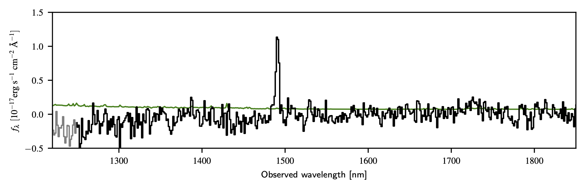
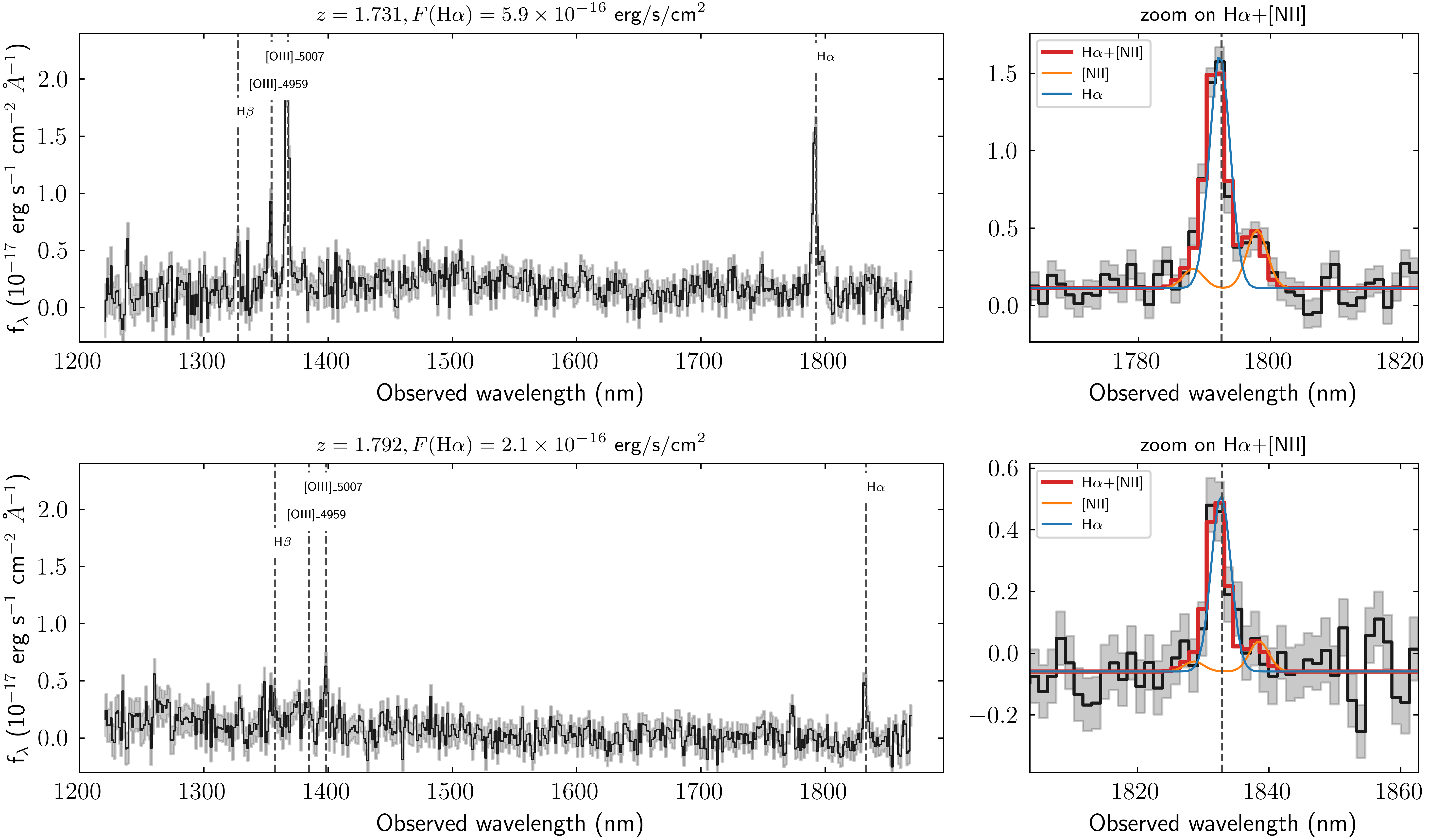
The goal of the EWS survey is to compute clustering statistics for galaxies in the range , using detections of the line at to secure their redshifts. For the present paper, however, we shall work with a slightly more conservative selection specific to Q1: . This constraint will be relaxed in future releases. The requirement, as defined in the original design of the survey, is that within this target range SPE PF shall deliver a sample that is 45% complete and 80% pure, for objects with an line detected with a signal-to-noise ratio (S/N) greater than 3.5, for sources with FWHM arcsec (since the spectral resolution depends on the size of the object along the dispersion direction). SPE PF therefore has to supplement the measured redshifts with all the information on the measurement quality required to select a catalogue within the target range. This means supplying the correct redshift for at least 45% of the full population of emitters matching the selection criteria, as well as a percentage of less than 20% of spurious objects with incorrect redshifts. Given the wavelength coverage of NISP and the exposure time, is the only line detected with good S/N for a large fraction of this redshift range and for a large fraction of targeted galaxies. In addition, the continuum is barely detected, such that a galaxy at redshift with and an line with flux has a typical spectrum as shown in Fig. 2.
The problem is that, when using an agnostic line identification tool, the emission line in this case is not identified as , but is incorrectly interpreted as [O ii]. In order to circumvent this issue, SPE PF introduces a prior in the calculation of the PDF, which favours solutions containing the line. The prior acts on the PDF by dividing its value by a parameterisable factor for redshifts at which the line can be detected. It currently has a value of 1000 below and above , where is not observed by the EWS, and unity for , where it is.
We thus ensure that, for objects such as the one shown in Fig. 2, the redshift solution favoured by SPE is the correct one. Of course, sometimes this will induce the opposite effect: real [O ii] emission lines can be wrongly identified as . However, to enter the red grism wavelength range, the [O ii] doublet at 3728 Å needs to come from a galaxy at . At the limiting magnitude of the EWS, the number of such galaxies is lower than that of true emitters within the target range by a factor of about 3.5 (as estimated from the EL-COSMOS data set; Saito et al. 2020) and the net result is thus an improvement of the redshift measurement success rate.
2.3 Reliability of the redshift estimation
Associated with each solution, the spe_z_prob parameter gives the value of the integral of the PDF under the corresponding peak, over a interval around the central value, where is the width of the Gaussian fit to the peak. This provides an indicator of the reliability of the redshift estimate: a spectrum with two or more strong coherent emission lines will typically yield a PDF with a single peak whose integral is close to unity. Conversely, a spectrum such as the one in Fig. 2 will typically induce a PDF with multiple peaks, each corresponding to different potential identifications of the line. In this case, the integral of the PDF is shared among the peaks, leading to lower associated probabilities. Finally, for a spectrum without any prominent feature, the PDF will contain many faint peaks corresponding mostly to noise fluctuations, and the probability associated with each solution will be low.
The results on the success rate of the observed samples (described in Sect. 6) show that the spe_z_prob parameter is highly nonlinear and that values below about 0.99 correspond to unreliable solutions. Improvements of the reliability of the redshift estimations are under development using machine-learning algorithms that will evaluate the whole shape of the PDF rather than a single peak. However, training of these algorithms requires a large sample of objects with secure redshifts, which will be provided by measurements on the EDS. An alternative will be to use simulated data, provided that they are sufficiently representative of the real spectra.
3 Redshift estimate performance
3.1 Comparison with external redshift measurements
In future Euclid public releases, the completeness and purity of galaxy samples for cosmological investigations will be quantified using the EDS as a reference. This will provide us with an internal, fully self-consistent control sample, to quantify redshift measurement systematics that can affect galaxy clustering and the resulting inferred cosmological parameters. Lacking such an internal reference and given the broader nature of the Q1 data set, to test the quality and limitations of the released data we need here to revert to external measurements. The only appropriate data set, in terms of area and redshift coverage, is provided by the Dark Energy Spectroscopic Instrument (DESI) Early Data Release catalogue (DESI Collaboration: Adame et al. 2024), which partly covers the EDF-N.
Within the DESI catalogue, we first selected objects with a reliable redshift, corresponding to: (1) quality flag z_warn (no issue identified in the redshift measurement); and (2) Delta_chi2 , which ensures that there is a significant difference between the main solution and the second one. The resulting sample was then matched to Euclid objects featuring three or more spectroscopic dithers and a reliable detection in the MER catalogue, using a matching radius of . This produced a sample of 25 469 matched objects. In the DESI catalogue, 10 885 of these are identified as stars, 985 as quasars, and 13 599 as galaxies.
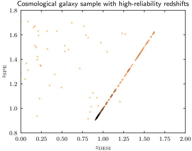
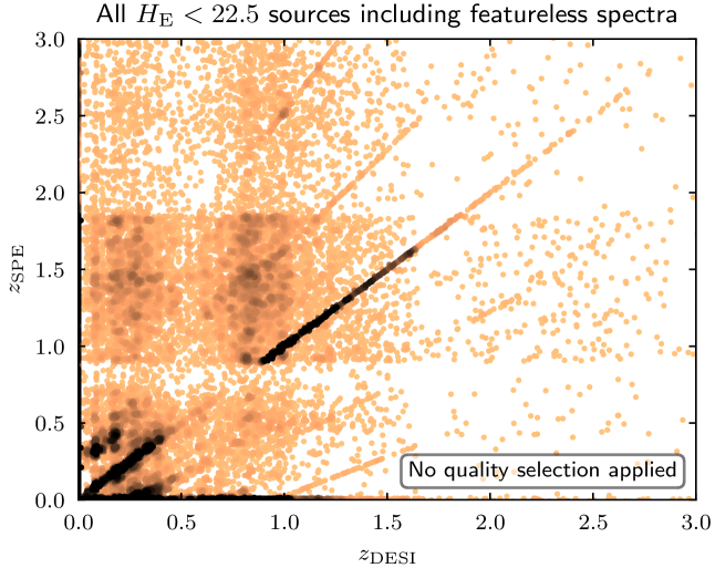
Figures 3 and 4 compare the DESI and SPE redshift measurements, for various quality selections. Figure 3 gives a first view of the quality of a Euclid ‘cosmological sample’ of emitting galaxies, selected within the reference flux and redshift limits. This plot directly proves the current ability of SPE to recover redshifts for those galaxies that are the targets for which Euclid NISP was built. A more in-depth discussion of this selection is presented in Sect. 6.2.
In the remainder of this section, we focus on the two panels of Fig. 4, which deliberately look at the data for any kind of object, varying the quality thresholds. The scope here is to test the ability of Euclid and the SPE pipeline in particular to work out of their ‘comfort zone’ and recover information beyond the cosmological goals NISP was designed for. The matched DESI sample includes in fact also galaxies outside the visibility range, for which the spectral characterisation has to be based on emission lines other than or on the continuum; there are also stars, for which some information can also be present in terms of absorption lines.
In the upper panel of Fig. 4, the effects of the previously discussed prior are easily noticeable as an overdensity of points in the region. Here, no quality criteria are applied, in order to give a full illustration of the various artefacts that can affect the performance of PF SPE, in particular when dealing with measurements outside the target redshift range.
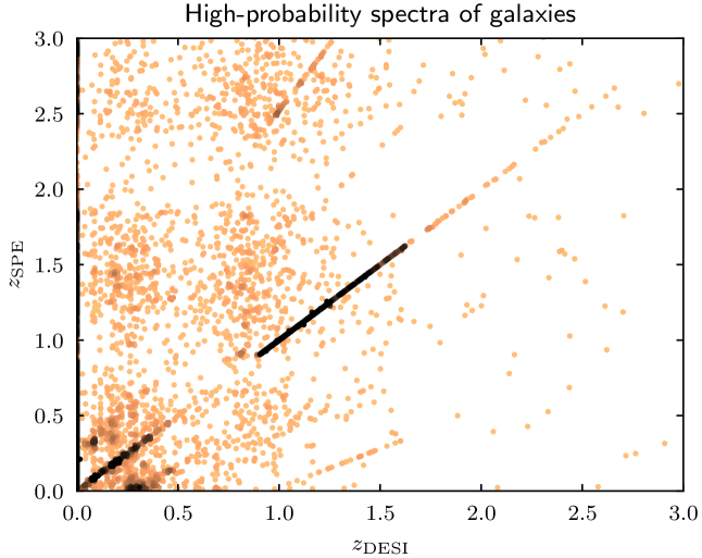
The bottom panel displays the same information, but only for galaxies with spe_z_proba, showing the relative efficiency of this selection in excluding incorrect solutions. It must be noted as well that, even if the percentage of correct solutions is low in the 0 – 0.9 interval (see Sect. 6 for detailed numbers), about 15% of galaxies measured by DESI in this redshift interval have a redshift measured by SPE in the same interval with spe_z_proba. Considering that the redshifts measured by SPE cannot rely on any strong emission lines except for specific categories (such as AGN), these measurements are solely based on a small portion of the continuum. This is nevertheless interesting, since NISP and the EWS were designed to measure redshifts for emitting galaxies at , and limited performance is expected below this redshift.
3.2 Redshift measurement uncertainties
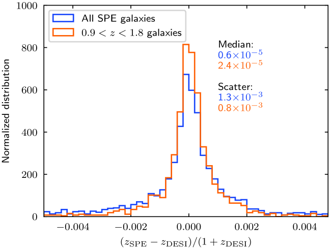
To evaluate the precision of Euclid redshifts, we computed the relative redshift difference between the redshift measured by SPE, for objects classified as galaxies and the one provided by DESI. After excluding outliers, defined as those having an absolute difference larger than 0.005, we obtain a distribution with a median value of and a dispersion of , which is plotted in Fig. 5. This provides an upper limit on the Euclid redshift uncertainties, since this quantity also contains the DESI uncertainties. However, with the DESI resolution ranging between 2000 and 5500, i.e., 4–5 times better than NISP, Euclid errors should dominate this comparison. If we restrict the sample to galaxies within the Euclid target range (, but no flux restriction), to ensure that at least the emission line is used for the redshift determination if it is present, the RMS error drops to , with a median value of . If we additionally cut the sample at the nominal flux limit of , the dispersion further reduces to . Given the low resolution of NISP and the sizeable spectroscopic undersampling, this remarkable agreement confirms the quality of the wavelength calibration, as described in Euclid Collaboration: Copin et al. (2025).
3.3 Types of redshift failure
As shown in Fig. 4, a significant fraction of galaxies have an incorrect redshift if only basic quality criteria are applied, and are thus not located on the one-to-one relation. There are two types of incorrect redshift visible in this figure.
A first type, which in the forthcoming Risso et al. (in prep.) paper are called ‘line interlopers’, is caused by the misidentification of a detected line. As already explained in Sect. 2.2, the SPE pipeline can attribute the wrong line to a feature. This is particularly the case if only one line can be seen in the Euclid spectral range. In this situation, the relation between the true redshift and wrong redshift is
| (1) |
where and are the true and wrong (misidentified) rest-frame wavelengths of the measured line, respectively. In Fig. 4, we see the signature of a few possible line misidentifications as the linear tracks off the main diagonal of the plot. Clearly, if all redshifts in the Q1 release are used without any quality filter (bottom panel of Fig. 4), a large variety of misidentifications are possible.
If, as in the bottom panel, we select high-quality SPE galaxies (defined as having spe_z_proba and a line width – expressed in terms of velocity dispersion – smaller than 680 km s-1 to exclude spurious broad features), we are left with three such features indicating line misidentifications. The one above the one-to-one diagonal corresponds to : this results from cases where SPE has interpreted a line as [O ii] when in fact it is . We can also notice two discrete features below the one-to-one relation, corresponding to being misidentified as , , or [S iii]9530, . Finally, inspection of the histogram reveals the presence of a small peak at 1.34, corresponding to being misidentified as , although we surprisingly do not find the peak corresponding to [O iii].
As can be seen by comparing with Fig. 3, such misidentifications are largely suppressed by the prior, and this aspect will be revisited in future versions of the pipeline. We remark that no obvious misidentification is observed in the target redshift range for cosmology, –1.8.
The second type of error (giving rise to what we call ‘noise interlopers’ in Risso et al. 2025) is caused by noise features or pipeline artefacts, such as unflagged residuals of the zeroth order signal, which are mistaken for real lines. In such cases, the measured redshift values are spread over a broad range. However, they are less likely to happen for redshift ranges where two real lines fall within the nominal NISP wavelength range, since this would require two spurious peaks separated by the same exact wavelength difference of two emission lines (this is the case in the range when considering [O iii]5007 and ). Conversely, the prior tends to push these spurious redshifts into the cosmology target range. As a result, the distribution of these incorrect redshifts is not uniform, as shown in Fig. 4.
4 Spectral classification
In addition to the redshift, SPE also provides classifications into three main types: galaxies, stars, and quasars. We compared these classifications in the EDF-N with the DESI ones. In Table 1, we present the confusion matrix of the SPE classifier, which describes how the objects from a given ‘true’ class are classified into the various classes by the classifier. For a perfect classifier, we would have 100% on the diagonal and 0% everywhere else. We assume here that DESI is the ground truth, which could lead to biases in the estimate of the confusion matrix.
We consider two different cases. For the first, we select high-quality spectra with three or more dithers on average (see Sect. 2.1). For the second case, we additionally require a class probability higher than 0.99. The results are not significantly better for the second case. This suggests that the spectral quality and the SPE classification probability criteria alone cannot yet efficiently select objects with a good classification.
The results are satisfactory for galaxies, with around 80% success. The results for quasars are poor, with about 80% of them being classified as galaxies. The current version of the pipeline uses a single template for quasars based on the average spectrum of the SDSS quasars. It thus allows too little flexibility to fit the Euclid spectra reliably. In addition, this template has broad lines, and type II observed AGN tend to be fitted better by the galaxy templates, for example when the line-spread function is even slightly overestimated.
Only about 50% of the stars are correctly classified, while the remaining 50% leak into the galaxy class. Only 23% of these false galaxies are at , and 21% of them are in the target redshift range for cosmology (). This emphasises the fact that additional non-SPE criteria will be necessary to minimise the contamination of the cosmological sample by stars, and the high quality imaging of the Euclid space telescope will undoubtedly be efficient in doing this. In contrast, about 75% of the objects classified as stars by SPE are DESI stars. The selection of star samples is thus very promising, and the combination with other quality criteria from the Euclid photometric segment should provide high-quality samples.
| Classified by SPE as: | galaxies | stars | quasars |
|---|---|---|---|
| High-quality Euclid spectra | |||
| (3 dithers in average) | |||
| DESI galaxies | 80% | 12% | 8% |
| DESI stars | 49% | 49% | 2% |
| DESI quasars | 77% | 7% | 16% |
| High-quality Euclid spectra and | |||
| SPE classification probability 0.99 | |||
| DESI galaxies | 84% | 10% | 6% |
| DESI stars | 49% | 50% | 1% |
| DESI quasars | 79% | 7% | 14% |
5 Line-flux measurement products and performance
Once a redshift solution has been estimated for the galaxy model, the fluxes of all emission and absorption lines that are expected to be present in the spectrum are measured. It must be noted that for this Q1 release, even if an object is classified as a quasar or a star, the lines are identified at the redshift of the galaxy solution and therefore should not be trusted; this will be modified in future releases. Line fluxes are measured with two methods: ‘Direct Integration’ provides fluxes integrating the values of all the pixels of the emission line above the continuum; and ‘Gaussian Fit’ derives them from the fit of the line using a single, double, or multiple Gaussian model, depending on the line considered. Given the low spectral resolution of NISP, the and [N ii] doublet lines Direct-Integration fluxes are measured jointly over a unique wavelength interval to produce a single flux measurement, while the Gaussian Fit provides fluxes separately for the and [N ii] doublet. Examples of the fitting procedure results are displayed in Fig. 6 for a high S/N emission line, as well as for one close to the flux detection limit.
For each line and each method, SPE provides the flux, the S/N, the central wavelength and the full width at half maximum. All measurements relative to emission lines are stored in the spectro_line_features_catalog_spe_line_features_cat table: for each object, this contains all the detected lines for each redshift solution. A given line can be identified either by its name (e.g., Halpha) or a numerical identifier, and the link between line names and identifiers is given in the spectro_model_catalog_spe_lines_catalog table. Therefore, to retrieve the flux of the line for the main redshift solution of all objects, the selection should include spe_line_name=‘Halpha’ and spe_rank=0, together with any additional conditions.
A S/N value of 0.0 indicates that the measurement is unreliable, either due to unrealistically small value of the measured flux or to the fact that the flux measurement is made over a single valid pixel. Excluding those doubtful measurements, there are 272 676 objects for which the line is formally detected and has a flux measured with the Gaussian-Fit method greater than . This value is the limit under which no measurement can be performed, the limit for a detection being much higher: in the interval –, the average S/N is 6, with a dispersion of , meaning that more than 70% of these lines are detected with . This value is obtained with all the lines identified as whatever the quality of the measurement. For objects with z_spe_proba, the average value of the S/N rises to 6.7.
6 Success rates
Using the DESI redshifts in the EDF-N as a reference, we can estimate the success rate of SPE redshift measurements. Since the DESI redshift distribution is biased towards lower redshifts and brighter objects than for the objects targeted by Euclid, the results must be taken with caution, as discussed in Sect. 3.1. A better internal assessment will be possible at DR1, when a subset of the EDS (Euclid Collaboration: Scaramella et al. 2022) will be available. The full EDS will benefit from 15 multiple Wide-like red grism (1206–1892 Å) visits, supplemented by a further 25 visits with the blue grism (900–1300 Å). This has been designed as to retrieve virtually pure and complete reference samples, at the EWS depth (thanks to larger sensitivity), minimal spectral confusion between adjacent objects (thanks to multiple observing angles), and reduced redshift degeneracies (thanks to the extended blue-plus-red wavelength range). We will therefore have a reliable and complete control sample to calibrate EWS observations – including measurements of fluxes, which will allow a proper estimate of the completeness. In addition, realistic simulations will also be released along with DR1.
To obtain a quantitative estimate of the success rate, relative to the DESI sample, we compute the fraction of objects with in various sub-samples. This range corresponds to the nominal interval around SPE measurements. We focus on the range , i.e., the usual cosmological target range of Euclid, where falls within the red grism, but limited to , corresponding to the upper cut-off of the DESI sample. In the following sections, we study the dependence of the success rate as a function of the SPE redshift-probability threshold (gal_spe_z_prob). As expected, a high threshold produces a more reliable sample. However, this reduces the size of the recovered sample and thus the completeness, which cannot be estimated yet in the absence of full-depth EDFs, and the cutoff in magnitude.
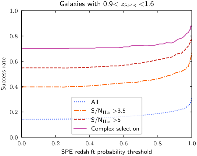
6.1 Success rate for non-cosmological science
The success rate for various quality selections is shown in Fig. 7. In the absence of any additional selection (blue), the reliability goes from 14% for a null SPE redshift probability threshold to 27% for a 0.99 threshold. The results can be improved dramatically by adding S/N criteria (3.5 in orange and 5 in red). With these additional criteria, we reach 61% and 75% success rates for a 0.99 probability threshold and S/N thresholds of 3.5 and 5, respectively. Finally, we add additional criteria on the flux and the width of the line found by template fitting. We keep only the sources with flux larger than , and also discard all objects for which the estimated line width saturates at the maximum value of the allowed range (), which is a signal of a spurious broad feature mistaken as emission line. With this selection, we reach a success rate of 85% for a threshold.
We also studied the SPE success rate outside the redshift range where can be detected. In Table 2, we summarise the performance obtained in various redshift slices. If we consider all three classes of objects and use a 0.99 redshift probability threshold for the best class, we reach a success rate of 53% at low () without adding any additional criteria. This result is encouraging, but it falls to only 7% if we select objects classified as galaxies, and we see that the apparently good results are mainly driven by stars (see Sect. 4). Not surprisingly, the results are also poor at , with an 8% success rate, explained mainly by the absence of any strong spectral features in the red-grism wavelength range. The performance is even poorer above , with a 2% success rate. This result is not so surprising, since no bright spectral feature is expected to be detected in the red grism above given the sensitivity of NISP.
Our results illustrate the importance of applying appropriate selection criteria when using spectroscopic data from the Q1 release. Measurements for galaxies in the Euclid target redshift range, where is covered by the red grism provide encouraging results. The same is true for stars. Outside of this redshift range, SPE results alone cannot be used to build a reasonably pure redshift sample for statistical studies; they must be complemented with additional data such as photometry (Cagliari et al. 2024) or morphological criteria that will be provided by the high quality Euclid images. A visual inspection of the spectra can also help to refine small samples for specific studies (Euclid collaboration: Quai et al. in prep.).
| Measured redshift | Success rate | ||
|---|---|---|---|
| 0.9 | 0.99 | 0.999 | |
| All the objects | |||
| 47% | 53% | 58% | |
| % | 8% | 8% | 8% |
| 27% | 34% | 38% | |
| 24% | 31% | 35% | |
| 2% | 2% | 3% | |
| Objects classified as galaxies only | |||
| 6% | 7% | 8%% | |
| 8% | 8% | 8% | |
| 26% | 33% | 37% | |
| 24% | 30% | 35% | |
| 2% | 2% | 2% | |
| Cosmological galaxy sample (SPE classification) | |||
| 64% | 75% | 82% | |
| 59% | 71% | 78% | |
| Cosmological sample (galaxies only in input) | |||
| 72% | 83% | 89% | |
| 67% | 78% | 85% | |
6.2 Success rate for cosmology goals
The measurement of reliable redshifts between and is the first crucial step towards Euclid’s cosmological goals based on galaxy clustering measurements. Although we do not have a true reference sample to test the cosmological performance, we can nevertheless draw useful indications by properly trimming the Q1 and DESI samples. We thus selected a galaxy sample similar to the baseline cosmological sample: flux larger than 2 and . In addition, we kept only objects for which the line width is narrower than the prior limit of to exclude artefacts (Sect. 3). The size limit of is not included in this study, and even better results could be obtained by adding this criterion.
In Fig. 3, we compare the redshift obtained by SPE and by DESI for the selection described in the previous paragraph and a SPE redshift probability larger than 0.99. Since the Euclid selection for cosmology is based on the measured line, the measured redshifts are all between 0.9 and 1.8. The results are dramatically improved compared to simpler selections discussed in Sect. 3 with most of the galaxies on the 1:1 relation. However, we also find a small population of galaxies with a lower DESI redshift, while only one object has a higher DESI redshift. Since they are not aligned, we can reasonably assume that these are spurious SPE redshifts that do not arise from simple line misidentifications. These sources erroneously measured by SPE at presumably arise from noise in the Euclid red-grism spectral range, and it is not surprising to have a small fraction of such spurious redshifts out of the large population of galaxies with and (see Sect. 2.1).
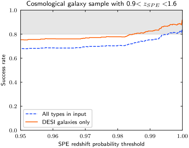
In Fig. 8, we present the SPE success rate as a function of the redshift properties for galaxies with measured properties matching the criteria of the cosmological sample. As explained in Sect. 6.1, we consider only the range, where both DESI and SPE are reliable. If we select galaxies based on the SPE classification only, we reach an 80 % success rate for z_spe_proba (blue dashed line). However, the SPE-only classification is not highly reliable (Sect. 4), and we will eventually benefit from Euclid morphological and photometric information to discard stars and lower redshift galaxies from the sample. To obtain a performance forecast closer to the expected methods that will be used in Euclid, we computed the success rate for a clean sample classified by both SPE and DESI as galaxies. A z_spe_proba threshold of 0.985 is enough to obtain an 80% success rate, and we can reach 89% for a stringent z_spe_proba criterion.
In short, we have demonstrated that success rates higher than the specifications (see Table 2 for a summary) can be obtained for the cosmological sample if we select the sample carefully. For the future Euclid DR1, further adjustments will be possible in order to establish the optimal threshold that yields the best compromise between success rate and sample size, in order to maximise the performance for cosmology. These future analyses will use the EDS data, which are not part of the Q1.
7 Conclusions
We have presented the first data release (Q1) of the SPE PF results. If we properly combine the various quality indicators provided by the pipeline, we showed that we can reach a success rate above 80% in the redshift range targeted for cosmology (). The redshift precision (approximately ) and accuracy (better than ) are also excellent. This is encouraging for the future DR1 and the first cosmological results, but the completeness will still need to be assessed when EDS data will be available and all EWS sources down to instead of 22.5 will have been processed.
As would be expected, the results are less good outside of this redshift range, since no strong spectral features are then observable within the NISP red-grism spectral range, and these data should be used with caution for non-cosmology science. Future deep-field observations including the blue grism should dramatically improve Euclid’s performance in this regime. In addition, the sample of star candidates selected by SPE PF based on spectroscopy alone is 75% pure. This is very promising for the study of cool stars (Banados et al., in prep.).
Finally, the current results are only a first step and we can expect major improvements in the future. The PF-SIR products injected into SPE PF still contain important artefacts (Euclid Collaboration: Copin et al. 2025), which will be corrected in the next versions of the pipeline. This should dramatically reduce the fraction of spurious redshifts and enable us to use less stringent selection criteria, increasing the size of the high-reliability samples. The SPE PF pipeline itself will also improve. Deep-learning approaches have been developed to estimate the redshift reliability and classify the spectra. We already trained and tested such algorithms on simulations and they outperformed the current algorithm. However, we will need future real EDS data to build a proper training set for the analysis of real EWS data. Finally, the selection of galaxies for cosmological analyses will also benefit from non-spectroscopic information (e.g., morphology or photometry), allowing us to obtain sufficiently pure and complete samples.
Acknowledgements.
This work has made use of the Euclid Quick Release Q1 data from the Euclid mission of the European Space Agency (ESA), 2025, https://doi.org/10.57780/esa-2853f3b. The Euclid Consortium acknowledges the European Space Agency and a number of agencies and institutes that have supported the development of Euclid, in particular the Agenzia Spaziale Italiana, the Austrian Forschungsförderungsgesellschaft funded through BMK, the Belgian Science Policy, the Canadian Euclid Consortium, the Deutsches Zentrum für Luft- und Raumfahrt, the DTU Space and the Niels Bohr Institute in Denmark, the French Centre National d’Etudes Spatiales, the Fundação para a Ciência e a Tecnologia, the Hungarian Academy of Sciences, the Ministerio de Ciencia, Innovación y Universidades, the National Aeronautics and Space Administration, the National Astronomical Observatory of Japan, the Netherlandse Onderzoekschool Voor Astronomie, the Norwegian Space Agency, the Research Council of Finland, the Romanian Space Agency, the State Secretariat for Education, Research, and Innovation (SERI) at the Swiss Space Office (SSO), and the United Kingdom Space Agency. A complete and detailed list is available on the Euclid web site (www.euclid-ec.org). This research used data obtained with the Dark Energy Spectroscopic Instrument (DESI). DESI construction and operations is managed by the Lawrence Berkeley National Laboratory. This material is based upon work supported by the U.S. Department of Energy, Office of Science, Office of High-Energy Physics, under Contract No. DEAC0205CH11231, and by the National Energy Research Scientific Computing Center, a DOE Office of Science User Facility under the same contract. Additional support for DESI was provided by the U.S. National Science Foundation (NSF), Division of Astronomical Sciences under Contract No. AST-0950945 to the NSFs National Optical-Infrared Astronomy Research Laboratory; the Science and Technology Facilities Council of the United Kingdom; the Gordon and Betty Moore Foundation; the Heising-Simons Foundation; the French Alternative Energies and Atomic Energy Commission (CEA); the National Council of Science and Technology of Mexico (CONACYT); the Ministry of Science and Innovation of Spain (MICINN), and by the DESI Member Institutions: www.desi.lbl.gov/collaborating-institutions. The DESI collaboration is honoured to be permitted to conduct scientific research on Iolkam Duag (Kitt Peak), a mountain with particular significance to the Tohono Oodham Nation. Any opinions, findings, and conclusions or recommendations expressed in this material are those of the author(s) and do not necessarily reflect the views of the U.S. National Science Foundation, the U.S. Department of Energy, or any of the listed funding agencies.References
- Bruzual & Charlot (2003) Bruzual, G. & Charlot, S. 2003, MNRAS, 344, 1000
- Cagliari et al. (2024) Cagliari, M. S., Granett, B. R., Guzzo, L., et al. 2024, A&A, 689, A166
- DESI Collaboration: Adame et al. (2024) DESI Collaboration: Adame, A. G., Aguilar, J., Ahlen, S., et al. 2024, AJ, 168, 58
- Euclid Collaboration: Aussel et al. (2025) Euclid Collaboration: Aussel, H., Tereno, I., Schirmer, M., et al. 2025, A&A, submitted
- Euclid Collaboration: Copin et al. (2025) Euclid Collaboration: Copin, Y., Fumana, M., Mancini, C., et al. 2025, A&A, submitted
- Euclid Collaboration: Cropper et al. (2024) Euclid Collaboration: Cropper, M., Al Bahlawan, A., Amiaux, J., et al. 2024, A&A, accepted, arXiv:2405.13492
- Euclid Collaboration: Jahnke et al. (2024) Euclid Collaboration: Jahnke, K., Gillard, W., Schirmer, M., et al. 2024, A&A, accepted, arXiv:2405.13493
- Euclid Collaboration: Mellier et al. (2024) Euclid Collaboration: Mellier, Y., Abdurro’uf, Acevedo Barroso, J., et al. 2024, A&A, accepted, arXiv:2405.13491
- Euclid Collaboration: Polenta et al. (2025) Euclid Collaboration: Polenta, G., Frailis, M., Alavi, A., et al. 2025, A&A, submitted
- Euclid Collaboration: Romelli et al. (2025) Euclid Collaboration: Romelli, E., Kümmel, M., Dole, H., et al. 2025, A&A, submitted
- Euclid Collaboration: Scaramella et al. (2022) Euclid Collaboration: Scaramella, R., Amiaux, J., Mellier, Y., et al. 2022, A&A, 662, A112
- Euclid Quick Release Q1 (2025) Euclid Quick Release Q1. 2025, https://doi.org/10.57780/esa-2853f3b
- Le Fvre et al. (2013) Le Fvre, O., Cassata, P., Cucciati, O., et al. 2013, A&A, 559, A14
- Pickles (1998) Pickles, A. J. 1998, PASP, 110, 863
- Risso et al. (2025) Risso, I., Veropalumbo, A., Branchini, E., et al. 2025, A&A, to be submitted
- Saito et al. (2020) Saito, S., delaTorre, S., Ilbert, O., et al. 2020, MNRAS, 494, 199
- Schmitt et al. (2019) Schmitt, A., Arnouts, S., Borges, R., et al. 2019, in ASP Conf. Ser., Vol. 521, Astronomical Data Analysis Software and Systems XXVI, ed. M. Molinaro, K. Shortridge, & F. Pasian, 398
- Vanden Berk et al. (2001) Vanden Berk, D. E., Richards, G. T., Bauer, A., et al. 2001, AJ, 122, 549