EUDA: An Efficient Unsupervised Domain Adaptation via Self-Supervised Vision Transformer
Abstract
Unsupervised domain adaptation (UDA) aims to mitigate the domain shift issue, where the distribution of training (source) data differs from that of testing (target) data. Many models have been developed to tackle this problem, and recently vision transformers (ViTs) have shown promising results. However, the complexity and large number of trainable parameters of ViTs restrict their deployment in practical applications. This underscores the need for an efficient model that not only reduces trainable parameters but also allows for adjustable complexity based on specific needs while delivering comparable performance. To achieve this, in this paper we introduce an Efficient Unsupervised Domain Adaptation (EUDA) framework. EUDA employs the DINOv2, which is a self-supervised ViT, as a feature extractor followed by a simplified bottleneck of fully connected layers to refine features for enhanced domain adaptation. Additionally, EUDA employs the synergistic domain alignment loss (SDAL), which integrates cross-entropy (CE) and maximum mean discrepancy (MMD) losses, to balance adaptation by minimizing classification errors in the source domain while aligning the source and target domain distributions. The experimental results indicate the effectiveness of EUDA in producing comparable results as compared with other state-of-the-art methods in domain adaptation with significantly fewer trainable parameters, between 42% to 99.7% fewer. This showcases the ability to train the model in a resource-limited environment. The code of the model is available at: https://github.com/A-Abedi/EUDA.
Index Terms:
Unsupervised domain adaptation, vision transformers, Max mean discrepancy, self-supervised LearningI Introduction
Unsupervised domain adaptation (UDA) has shown promising results in addressing the domain shift problem, where the distribution of the training data (source domain) differs from that of the test data (target domain), and knowledge transfer [1]. The domain shift problem can significantly degrade the performance of conventional deep neural networks (DNNs) when applied directly to the target domain [2]. UDA overcomes this issue by leveraging unlabeled data from the target domain to align feature distributions and enhance model adaptation [3]. Additionally, traditional DNNs often rely on a large number of annotated samples, which limits their applicability in conditions where labeling is expensive, such as autonomous driving [4]. UDA solves this problem by transferring knowledge from previously labeled data (source domain) to unlabeled data in the target domain, thereby enhancing model performance without the need for extensive new annotations.
Existing UDA methods can be classified into: (i) adversarial methods, which use generative adversarial networks to generate domain-invariant features [5, 6, 7]; (ii) reconstruction methods, which employ encoder-decoder structures to learn invariant features by reconstructing domains [8, 9]; (iii) transformation methods, which optimize inputs through transformations to enhance adaptation [10, 3]; and (iv) discrepancy methods, which align domain features through statistical metrics like maximum mean discrepancy (MMD) [11, 12, 13] and correlational alignment (CORAL) [14, 15]. Regardless of which UDA method is chosen, the backbone of the network for feature extraction plays a crucial role. The backbone is responsible for extracting features from the input data, and the more generalized and domain-invariant these features are, the better the UDA results will be. Recently, vision transformers (ViTs) [16] have revolutionized computer vision by adapting the transformer architecture, originally designed for natural language processing [17], to process images as sequences of patches. This approach enables ViTs to capture global image dependencies, offering a more comprehensive understanding than the local feature extraction typical of convolutional neural networks (CNNs) [18]. This capability makes ViTs well-suited for complex tasks such as object recognition and scene understanding [16] and particularly effective in UDA [19, 20, 21].
The success of ViTs in large-scale pre-training also shows significant performance improvements on benchmarks, particularly in UDA, making the integration of self-supervised learning (SSL) strategies effective [22, 23, 24]. SSL allows ViTs to learn detailed representations from vast, unlabeled datasets, enhancing generalization and robustness across various visual domains [25, 26, 22]. Among these methods, DINOv2 [24] stands out for its ability to extract general-purpose features [26, 24]. This positions DINOv2 as a powerful tool for advancing UDA, highlighting its transformative potential in modern visual computing.
Despite the promising performance of the state-of-the-art UDA models, they often follow complex frameworks. Particularly those utilizing ViT architectures as backbone, which involve a significant amount of learnable parameters. These parameters need powerful computational resources for training. This complexity not only increases the cost of deployment but also limits their applicability in environments with limited resources. Therefore, there is a critical need for UDA models that are inherently simpler and have fewer trainable parameters. Such models would ensure more stable training and better generalization, and offer the versatility to adjust their complexity based on specific task demands and the complexity of various applications. By achieving this, we can facilitate more efficient domain adaptation across a wider range of practical settings, making advanced UDA techniques more accessible and sustainable.
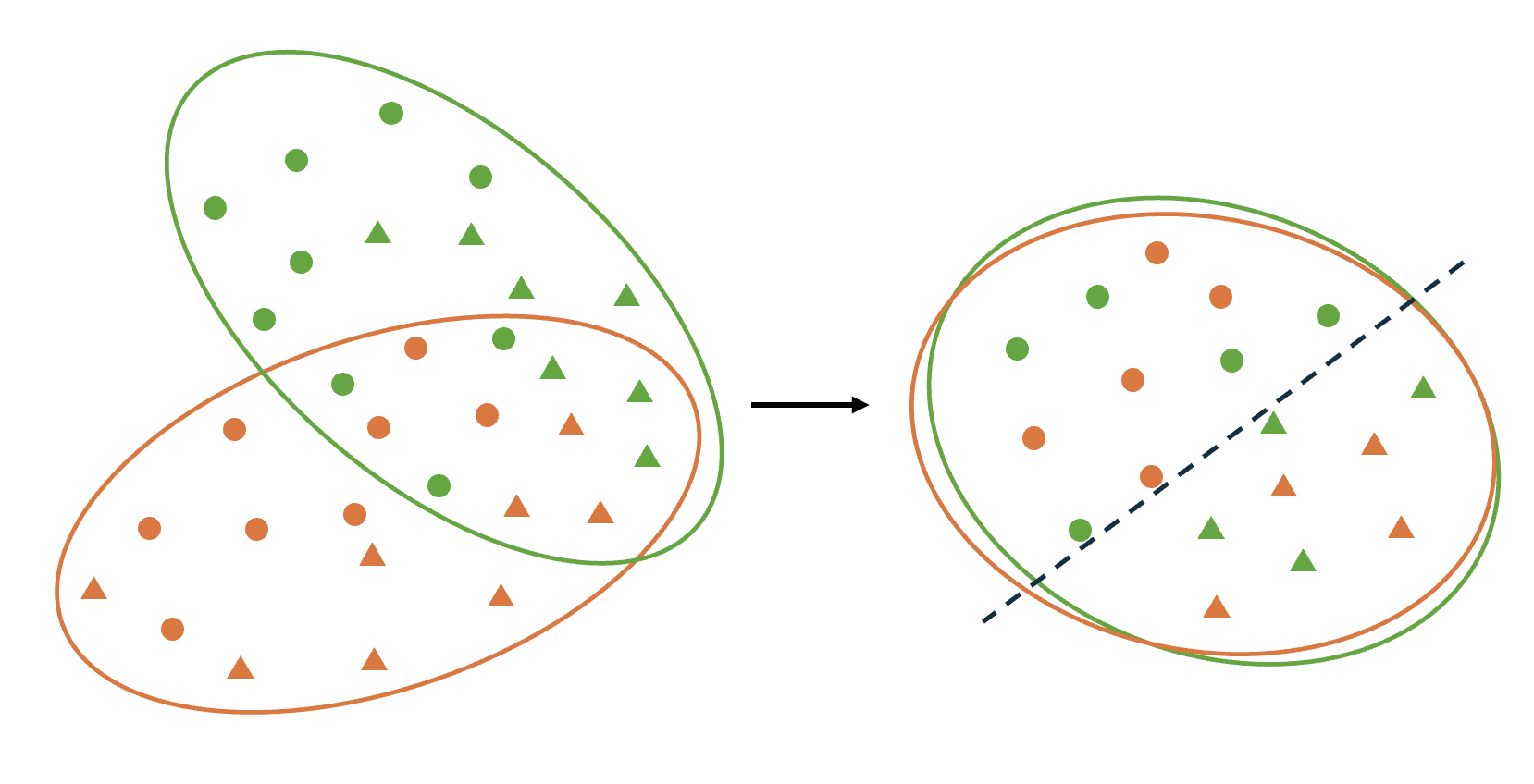
In this paper, we introduce a novel Efficient Unsupervised Domain Adaptation framework, known as EUDA, that utilizes the capabilities of self-supervised ViTs to address the challenges of UDA. Specifically, EUDA integrates DINOv2 as a feature extractor with a simple yet effective bottleneck consisting of fully connected layers. Using the fully connected layers aims to refine the features extracted by DINOv2 for effective domain adaptation. Additionally, inspired by [12] EUDA uses the synergistic domain alignment loss (SDAL), which combines cross-entropy (CE) loss and MMD loss. This hybrid loss function effectively balances the adaptation by minimizing classification errors on the source domain while aligning the distributions between the source and target domains, as shown in Fig. 1. By leveraging the self-supervised pre-training of DINOv2 and the computational efficiency of the MMD, our approach offers a promising solution to UDA. It reduces the dependency on large, complex models and extensive computational resources, making it not only effective but also suitable for real-world applications where adaptability and efficiency are crucial. To the best of our knowledge, this is the first application of DINOv2 within a UDA framework, marking a significant advancement in leveraging self-supervised learning techniques for addressing domain adaptation challenges.
In summary, the main contributions of this paper are as follows:
-
•
To the best of our knowledge, we are the first to apply DINOv2, a self-supervised vision transformer, for UDA, utilizing its strength to generate robust, domain-invariant features.
-
•
We propose EUDA (Efficient Unsupervised Domain Adaptation), a novel framework that leverages self-supervised ViTs and MMD to tackle the challenges of UDA. EUDA features a flexible architecture with a simple bottleneck of fully connected layers, which require significantly fewer parameters to be tuned and can be adjusted according to the complexity of the problem.
-
•
We perform comprehensive experiments and ablation studies to validate the effectiveness of our proposed method on multiple benchmarks.
The rest of this paper is organized as follows: Section II reviews UDA, ViTs, and self-supervised learning approaches within ViTs. Section III details the proposed EUDA model. The experimental results across various configurations are presented in Section IV. Finally, Section V concludes the paper with insights and implications of our findings.
II Related Work
II-A Unsupervised Domain Adaptation
As stated in the introduction, the domain shift problem is the major concern in UDA. Over the years, numerous methods have been developed to tackle this issue, aiming to enable effective model performance on the target domain without relying on labeled data [27]. Adversarial methods use adversarial training to create domain-invariant features. For example, DANN [5] leverages a gradient reversal layer that inverts the gradient sign during training. ADDA [6] trains a source encoder on labeled images, and mixes source and target images to confuse the discriminator. Adversarial methods are computationally intensive, often exhibit unstable training processes, and do not always guarantee accurate feature mapping.
Transformation methods enhance domain adaptation by pre-processing input samples to optimize their condition for model training. DDA [10] preprocesses input data to align signal-to-noise ratios and reduce domain shifts, while TransPar [3] applies the lottery ticket hypothesis to identify and adjust transferable network parameters for better cross-domain generalization. These approaches are simple and effective but may not capture all domain differences.
Reconstruction methods utilize an encoder-decoder setup to harmonize features across domains by reconstructing target domain images from source domain data. MTAE [8] utilized a multitask autoencoder to reconstruct images from multiple domains. DSNs [9] enhance model performance by dividing image representations into domain-specific and shared subspaces. This improves generalization and surpasses other adaptation methods. They usually face challenges with high computational costs, training instability, and potential overfitting to the source domain.
Discrepancy methods have emerged as particularly effective for UDA. DAN [12] embeds task-specific layer representations into a reproducing kernel Hilbert space (RKHS) and uses MMD to explicitly match the mean embeddings of different domain distributions. WeightedMMD [13] introduces a weighted MMD that incorporates class-specific auxiliary weights to address class weight bias in domain adaptation. This approach optimizes feature alignment between source and target domains by considering class prior distributions. Joint adaptation networks [28] align the joint distributions of multiple domain-specific layers across domains using a Joint MMD criterion to improve domain adaptation by considering the combined shift in input features and output labels.
II-B Vision Transformer
Transformers, initially introduced by Vaswani et al. [17], have demonstrated exceptional performance across various language tasks. The core of their success lies in the attention mechanism, which excels at capturing long-range dependencies. ViT [16] represents a groundbreaking approach to applying transformers in vision tasks. It treats images as sequences of fixed-size, non-overlapping patches. Unlike CNNs that depend on inductive biases such as locality and translation equivariance, ViT leverages the power of large-scale pre-training data and global context modeling. ViT offers a straightforward yet effective balance between accuracy and computational efficiency [18].
In the context of UDA, ViTs have demonstrated remarkable potential. TVT [19] introduces a transferability adaptation module to guide the attention mechanism and a discriminative clustering technique to enhance feature diversity. CDTrans [20] consists of a triple-branch structure with weight-sharing and cross-attention to align features from source and target domains, alongside a two-way center-aware pseudo labeling strategy to improve label quality. WinTR [29] uses two classification tokens within a transformer model to learn distinct domain mappings with domain-specific classifiers. This enhances the cross-domain knowledge transfer through source-guided label refinement and single-sided feature alignment. PMTrans [21] combines patches from both domains using game-theoretical principles, mixup losses, and attention maps for effective domain alignment and feature learning.
While these methods have shown promising performance in solving UDA problems, they typically rely on complex architectures with extensive trainable parameters and sophisticated training regimes, including multi-branch transformers, cross-attention, adversarial training, game-theoretical principles, and mixup losses. Furthermore, these models generally require training the entire network, resulting in a substantial computational burden. As a result, achieving promising outcomes necessitates extensive training on large-scale models, limiting their practical applicability in resource-constrained environments [19, 20, 21].
II-C Self-supervised Vision Transformer
SSL has revolutionized the field of computer vision by enabling models to learn effective representations from unlabeled data, eliminating the dependency on large annotated datasets. These models learn representations by performing pre-text tasks, such as rotation prediction [30] and image colorization [31], and then apply the learned representations to downstream tasks. In the context of ViTs, SSL has been pivotal in enhancing their ability to extract robust, domain-invariant features. Jigsaw-ViT [32] integrates the jigsaw puzzle-solving problem into vision transformer architectures for improving image classification. EsViT [33] utilizes a multi-stage Transformer architecture to reduce computational complexity and introduces a novel region-matching pre-training task.
Among recent advancements in SSL for ViTs, DINO [26] and DINOv2 [24] have notably enhanced SSL by scaling up ViTs to effectively match representations across different views of the same image. With improvements like automatic data curation and innovative loss functions, DINOv2 excels in stability and efficiency. It can learn domain-invariant features essential for image classification and other vision tasks. Its capacity to generate robust feature maps makes DINOv2 an excellent choice for a feature extractor and representation generator. Because of these properties, we use DINOv2 in this research to significantly boost performance and generalization across various domains.
III Methodology
III-A Problem Formulation
UDA aims to learn a function that performs well on an unlabeled target domain by leveraging information from a labeled source domain. Let and denote the input and label spaces, respectively, indicates the source domain data, where and represent the input-output pairs, and indicates the target domain data, where is the input samples without labels, and are the number of samples in the source and target domains, respectively. The goal of UDA is to train a model on labeled source data and unlabeled target data in such a way that it performs well on the predicting target data labels .
III-B Model Overview
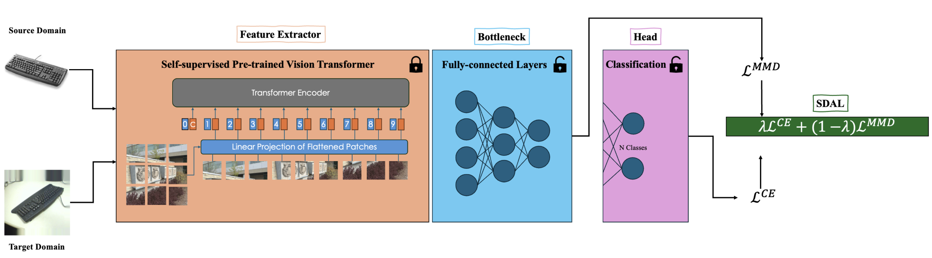
Fig. 2 shows an overview of our framework for addressing UDA problems. The model receives images from labeled source and unlabeled target domains. It then extracts features using a pre-trained self-supervised ViT, while its weights are frozen to ensure stability and efficiency. The extracted features from both domains are fed into a bottleneck composed of multiple fully connected layers to refine and condense the information. The bottleneck’s output serves a dual purpose. Firstly, it inputs into the classification head to compute the CE loss on source domain. Secondly, it contributes to the computation of the MMD loss to minimize the distance between source and target domain distributions in RKHS to align their feature representations. The pseudocode for our training procedure of EUDA is outlined in Algorithm 1. In the following subsections, we present different components of our model in detail.
III-C Feature Extractor
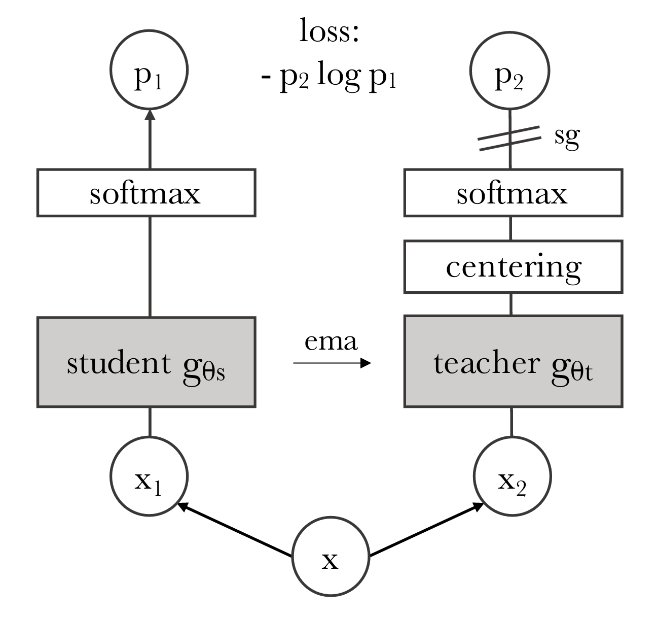
In our effort to leverage the capabilities of ViTs for domain adaptation, we adopt DINOv2 [24] as a self-supervised pre-trained model for feature extraction. It utilizes self-distillation to derive insights from unlabeled data autonomously. Central to DINOv2’s design is its twin-network structure, which includes a student and a teacher network. Both networks employ the same underlying architecture based on ViTs. During training, these networks process different augmentations of the same image. They aim to extract consistent features regardless of the input variations.
During the training phase (see Fig. 3), the student network’s parameters are continually updated, while the teacher network’s parameters are progressively updated through an exponential moving average of the student’s parameters. This ensures that the teacher model remains robust and generalizable. Moreover, DINOv2 uses registers [34] to improve the performance and interpretability of ViTs by addressing the problem of artifacts in feature maps, commonly observed in both supervised and self-supervised ViT networks. Registers are additional tokens added to the input sequence of ViTs to absorb high-norm token computations that typically occur in low-information areas of images.
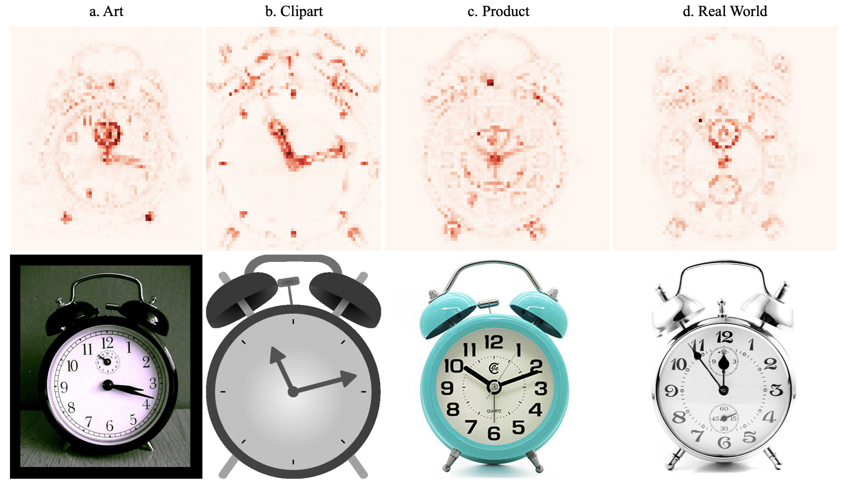
In our study, we leverage DINOv2 as the primary feature extractor due to its robust training on a large-scale, diverse dataset through self-supervised learning. To enhance efficiency, we freeze the model’s parameters. This approach reduces the computational burden and significantly decreases the number of trainable parameters. This makes our method notably more efficient compared to other UDA techniques that require extensive training. Consequently, our streamlined model is well-suited for deployment in real-world scenarios and on-edge devices, where computational resources are often limited. Fig. 4 shows the attention map of the pre-trained DINOv2 base model without any fine-tuning. This highlights its robustness across four different domains of the office-home [35] dataset. This demonstrates the precision and accuracy of the features extracted by DINOv2, underscoring the effectiveness of the EUDA feature extraction approach.
Using DINOv2 as the feature extractor significantly enhances our model by employing its robust, self-supervised pre-training to extract general-purpose features from images. The pre-trained DINOv2, with its weights frozen, ensures the extraction of high-quality features and reduces the number of trainable parameters. It can greatly simplify integration and adaptation in resource-limited settings, providing a strong foundation for effective domain adaptation.
III-D Bottleneck
The bottleneck component in our architecture consists of a series of fully connected layers. At the core of our model, the bottleneck output serves two primary functions. Firstly, it feeds into a classification head composed of a simple linear layer. This setup utilizes minimal computational resources to classify images efficiently. Secondly, the output acts as the feature vector for calculating the MMD loss, which aims to minimize the distance between source and target feature vectors. This facilitates effective domain adaptation.
The design of this dual-function bottleneck simplifies our model architecture and enhances its generalization capabilities across various domains. Its straightforward structure helps prevent overfitting, a frequent challenge in domain-specific applications, ensuring robustness for real-world deployments. Additionally, the minimalistic approach in the bottleneck design allows for easier maintenance and adaptability, which is crucial for meeting the dynamic requirements of domain adaptation tasks.
The bottleneck follows a simple yet efficient design for flexible adjustments in the model’s complexity. This flexibility allows us to adjust the model to meet specific performance needs or computational limits, which is particularly useful in settings with restricted resources.
III-E Synergistic Domain Alignment Loss
The SDAL is a composite loss function designed for the UDA models. It combines the strengths of CE loss and MMD loss. Formally defined as:
| (1) |
where and are the CE and MMD losses, respectively, and is a tunable hyperparameter that balances the influence of each loss component, it allows for a flexible adjustment according to specific domain adaptation needs.
CE loss is a widely used loss function in classification tasks. The CE loss increases as the predicted probability diverges from the actual label, thus providing a robust metric for optimizing classification models. The mathematical formulation of CE loss for a multi-class classification task is given by:
| (2) |
where is the number of samples, is the number of classes, is a one-hot vector indicating whether class label is the correct classification for the sample, and is the predicted probability of the th sample belonging to class . This formula penalizes the deviation of each predicted class probability from the actual class labels.
MMD loss is defined as the squared distance between the mean embeddings of features from the two domains in an RKHS [36]. The MMD loss can be written as:
| (3) |
where and denote the number of samples in the source and target domains, respectively, and are the data samples from these domains, and is a feature mapping function that projects the data into RKHS . By minimizing the MMD loss, we aim to align the statistical properties of the source and target domains.
| Model | Backbone | A C | A P | A R | C A | C P | C R | P A | P C | P R | R A | R C | R P | Avg. |
|---|---|---|---|---|---|---|---|---|---|---|---|---|---|---|
| Source Only | ResNet | 34.9 | 50.0 | 58.0 | 37.4 | 41.9 | 46.2 | 38.5 | 31.2 | 60.4 | 53.9 | 41.2 | 59.9 | 46.1 |
| RevGrad | ResNet | 45.6 | 59.3 | 70.1 | 47.0 | 58.5 | 60.9 | 46.1 | 43.7 | 68.5 | 63.2 | 51.8 | 76.8 | 57.6 |
| CDAN | ResNet | 50.7 | 70.6 | 76.0 | 57.6 | 70.0 | 70.0 | 57.4 | 50.9 | 77.3 | 70.9 | 56.7 | 81.6 | 65.8 |
| TADA | ResNet | 53.1 | 72.3 | 77.2 | 59.1 | 71.2 | 72.1 | 59.7 | 53.1 | 78.4 | 72.4 | 60.0 | 82.9 | 67.6 |
| SHOT | ResNet | 57.1 | 78.1 | 81.5 | 68.0 | 78.2 | 78.1 | 67.4 | 54.9 | 82.2 | 73.3 | 58.8 | 84.3 | 71.8 |
| Source Only | ViT (Deit) | 55.6 | 73.0 | 79.4 | 70.6 | 72.9 | 76.3 | 67.5 | 51.0 | 81.0 | 74.5 | 53.2 | 82.7 | 69.8 |
| Source Only | ViT | 66.16 | 84.28 | 86.64 | 77.92 | 83.28 | 84.32 | 75.98 | 62.73 | 88.66 | 80.10 | 66.19 | 88.65 | 78.74 |
| TVT - Baseline | ViT | 71.94 | 80.67 | 86.67 | 79.93 | 80.38 | 83.52 | 76.89 | 70.93 | 88.27 | 83.02 | 72.91 | 88.44 | 80.30 |
| CDTrans | ViT (Deit) | 68.8 | 85.0 | 86.9 | 81.5 | 87.1 | 87.3 | 79.6 | 63.3 | 88.2 | 82.0 | 66.0 | 90.6 | 80.5 |
| TVT | ViT | 74.89 | 86.82 | 89.47 | 82.78 | 87.95 | 88.27 | 79.81 | 71.94 | 90.13 | 85.46 | 74.62 | 90.56 | 83.56 |
| EUDA - LL (Ours) | ViT (DinoV2) | 80.6 | 84.9 | 88.4 | 85.2 | 88.0 | 88.6 | 76.6 | 77.4 | 86.7 | 87.7 | 82.5 | 92.8 | 84.9 |
| PMTrans | ViT | 81.2 | 91.6 | 92.4 | 88.9 | 91.6 | 93.0 | 88.5 | 80.0 | 93.4 | 89.5 | 82.4 | 94.5 | 88.9 |
| Model | Backbone | A W | D W | W D | A D | D A | W A | Avg. |
|---|---|---|---|---|---|---|---|---|
| Source Only | ResNet | 68.9 | 68.4 | 62.5 | 96.7 | 60.7 | 99.3 | 76.1 |
| RevGrad | ResNet | 82.0 | 96.9 | 99.1 | 79.7 | 68.2 | 67.4 | 82.2 |
| JAN | ResNet | 86.0 | 96.7 | 99.7 | 85.1 | 69.2 | 70.7 | 84.6 |
| CDAN | ResNet | 86.0 | 96.7 | 99.7 | 85.1 | 69.2 | 70.7 | 84.6 |
| SHOT | ResNet | 90.1 | 98.4 | 99.9 | 94.0 | 74.7 | 74.3 | 88.6 |
| Source Only | ViT (Deit) | 90.8 | 90.4 | 76.8 | 98.2 | 76.4 | 100.0 | 88.8 |
| Source Only | ViT | 89.2 | 98.9 | 100.0 | 88.8 | 80.1 | 79.8 | 89.5 |
| TVT - Baseline | ViT | 91.6 | 99.0 | 100.0 | 90.6 | 80.2 | 80.2 | 90.3 |
| TVT | ViT | 91.6 | 99.0 | 100.0 | 90.6 | 80.2 | 80.2 | 90.3 |
| EUDA - LL (Ours) | ViT (DinoV2) | 95.3 | 100.0 | 100.0 | 93.4 | 80.5 | 82.9 | 92.0 |
| CDTrans | ViT (Deit) | 97.0 | 96.7 | 81.1 | 99.0 | 81.9 | 100.0 | 92.6 |
| PMTrans | ViT | 99.1 | 99.6 | 100.0 | 99.4 | 85.7 | 86.3 | 95.0 |
The loss defined in Eq. (1) leverages the labeled data in the source domain to fine-tune the classification performance via CE loss while aligning the distribution of the source and target domain features through MMD. The synergy between these two loss components enhances the model’s ability to perform effectively across different domains. This makes SDAL suitable for real-world applications where domain shift is a significant challenge. Additionally, minimizing the distance between the source and target domain distributions ensures that the feature representations from both domains are closely aligned, facilitating smoother and more reliable domain adaptation. Empirical studies have shown that MMD effectively reduces domain shift and improves model performance across various tasks [11, 12].
IV Experimental Studies
IV-A Datasets
We examine the effectiveness of our proposed method across three benchmarks. These datasets include: Office-31 [37], which consists of 4,652 images from three domains: Amazon, Webcam, and DSLR, across 31 categories; Office-Home [35], which consists of 15,500 images spread over four domains: Art, Clipart, Products, and Real World, within 65 categories; VisDA-2017 [38], which includes 280,000 images from four domains: Caltech-256, ImageNet, ILSVRC2012, and PASCAL VOC 2012 as the source domain and real images as the target, belonging to 12 categories; and DomainNet [39], which consists of 48,129 images from six domains: Clipart, Real, Sketch, Infograph, Painting, and Quickdraw, across 345 categories.
| Model | Backbone | plane | bcycl | bus | car | house | knife | mcycl | person | plant | sktbrd | train | truck | Avg. |
|---|---|---|---|---|---|---|---|---|---|---|---|---|---|---|
| Source Only | ResNet | 55.1 | 53.3 | 61.9 | 59.1 | 80.6 | 17.9 | 79.7 | 31.2 | 81.0 | 26.5 | 73.5 | 8.5 | 52.4 |
| RevGrad | ResNet | 81.9 | 77.7 | 82.8 | 44.3 | 81.2 | 29.5 | 65.1 | 28.6 | 51.9 | 54.6 | 82.8 | 7.8 | 57.4 |
| BNM | ResNet | 89.6 | 61.5 | 76.9 | 55.0 | 89.3 | 69.1 | 81.3 | 65.5 | 90.0 | 47.3 | 89.1 | 30.1 | 70.4 |
| MCD | ResNet | 87.0 | 60.9 | 83.7 | 64.0 | 88.9 | 79.6 | 84.7 | 76.9 | 88.6 | 40.3 | 83.0 | 25.8 | 71.9 |
| SWD | ResNet | 90.8 | 82.5 | 81.7 | 70.5 | 91.7 | 69.5 | 86.3 | 77.5 | 87.4 | 63.6 | 85.6 | 29.2 | 76.4 |
| DTA | ResNet | 93.7 | 82.2 | 85.6 | 83.8 | 93.0 | 81.0 | 90.7 | 82.1 | 95.1 | 78.1 | 86.4 | 32.1 | 81.5 |
| SHOT | ResNet | 94.3 | 88.5 | 80.1 | 57.3 | 93.1 | 94.9 | 80.7 | 80.3 | 91.5 | 89.1 | 86.3 | 58.2 | 82.9 |
| Source Only | ViT (Deit) | 97.7 | 48.1 | 86.6 | 61.6 | 78.1 | 63.4 | 94.7 | 10.3 | 87.7 | 47.7 | 94.4 | 35.5 | 67.1 |
| Source Only | ViT | 98.2 | 73.0 | 82.6 | 62.0 | 97.4 | 63.6 | 96.5 | 29.8 | 68.8 | 86.8 | 96.8 | 23.7 | 73.3 |
| TVT - Baseline | ViT | 94.6 | 81.6 | 81.9 | 69.9 | 93.6 | 70.0 | 88.6 | 50.5 | 86.8 | 88.5 | 91.5 | 20.1 | 76.5 |
| EUDA - BH (Ours) | ViT (DinoV2) | 99.5 | 78.1 | 90.6 | 58.1 | 98.5 | 98.5 | 97.8 | 63.4 | 79.8 | 97.3 | 98.2 | 37.1 | 83.2 |
| TVT | ViT | 93.0 | 85.6 | 77.6 | 60.5 | 93.6 | 98.2 | 89.4 | 76.4 | 93.6 | 92.1 | 91.7 | 55.8 | 84.0 |
| PMTrans | ViT | 98.2 | 92.2 | 88.1 | 77.0 | 97.4 | 95.8 | 94.0 | 72.1 | 97.1 | 95.2 | 94.6 | 51.0 | 87.7 |
| CDTrans | ViT (Deit) | 97.1 | 90.5 | 82.4 | 77.5 | 96.6 | 96.1 | 93.6 | 88.6 | 97.9 | 86.9 | 90.3 | 62.8 | 88.4 |
| MCD | clp | inf | pnt | qdr | rel | skt | Avg. | SWD | clp | inf | pnt | qdr | rel | skt | Avg. | BNM | clp | inf | pnt | qdr | rel | skt | Avg. |
|---|---|---|---|---|---|---|---|---|---|---|---|---|---|---|---|---|---|---|---|---|---|---|---|
| clp | - | 15.4 | 25.5 | 3.3 | 44.6 | 31.2 | 24.0 | clp | - | 14.7 | 31.9 | 10.1 | 45.3 | 36.5 | 27.7 | clp | - | 12.1 | 33.1 | 6.2 | 50.8 | 40.2 | 28.5 |
| inf | 24.1 | - | 24.0 | 1.6 | 35.2 | 19.7 | 20.9 | inf | 22.9 | - | 24.2 | 2.5 | 33.2 | 21.3 | 20.0 | inf | 26.6 | - | 28.5 | 2.4 | 38.5 | 18.1 | 22.8 |
| pnt | 31.1 | 14.8 | - | 1.7 | 48.1 | 22.8 | 23.7 | pnt | 33.6 | 15.3 | - | 4.4 | 46.1 | 30.7 | 26.0 | pnt | 39.9 | 12.2 | - | 3.4 | 54.5 | 36.2 | 29.2 |
| qdr | 8.5 | 2.1 | 4.6 | - | 7.9 | 7.1 | 6.0 | qdr | 15.5 | 2.2 | 6.4 | - | 11.1 | 10.2 | 9.1 | qdr | 17.8 | 1.0 | 3.6 | - | 9.2 | 8.3 | 8.0 |
| rel | 39.4 | 17.8 | 41.2 | 1.5 | - | 25.2 | 25.0 | rel | 41.2 | 18.1 | 44.2 | 4.6 | - | 31.6 | 27.9 | rel | 48.6 | 13.2 | 49.7 | 3.6 | - | 33.9 | 29.8 |
| skt | 37.3 | 12.6 | 27.2 | 4.1 | 34.5 | - | 23.1 | skt | 44.2 | 15.2 | 37.3 | 10.3 | 44.7 | - | 30.3 | skt | 54.9 | 12.8 | 42.3 | 5.4 | 51.3 | - | 33.3 |
| Avg. | 28.1 | 12.5 | 24.5 | 2.4 | 34.1 | 21.2 | 20.5 | Avg. | 31.5 | 13.1 | 28.8 | 6.4 | 36.1 | 26.1 | 23.6 | Avg. | 37.6 | 10.3 | 31.4 | 4.2 | 40.9 | 27.3 | 25.3 |
| CGDM | clp | inf | pnt | qdr | rel | skt | Avg. | MDD | clp | inf | pnt | qdr | rel | skt | Avg. | SCDA | clp | inf | pnt | qdr | rel | skt | Avg. |
| clp | - | 16.9 | 35.3 | 10.8 | 53.5 | 36.9 | 30.7 | clp | - | 20.5 | 40.7 | 6.2 | 52.5 | 42.1 | 32.4 | clp | - | 18.6 | 39.3 | 5.1 | 55.0 | 44.1 | 32.4 |
| inf | 27.8 | - | 28.2 | 4.4 | 48.2 | 22.5 | 26.2 | inf | 33.0 | - | 33.8 | 2.6 | 46.2 | 24.5 | 28.0 | inf | 29.6 | - | 34.0 | 1.4 | 46.3 | 25.4 | 27.3 |
| pnt | 37.7 | 14.5 | - | 4.6 | 59.4 | 33.5 | 30.0 | pnt | 43.7 | 20.4 | - | 2.8 | 51.2 | 41.7 | 32.0 | pnt | 44.1 | 19.0 | - | 2.6 | 56.2 | 42.0 | 32.8 |
| qdr | 14.9 | 1.5 | 6.2 | - | 10.9 | 10.2 | 8.7 | qdr | 18.4 | 3.0 | 8.1 | - | 12.9 | 11.8 | 10.8 | qdr | 30.0 | 4.9 | 15.0 | - | 25.4 | 19.8 | 19.0 |
| rel | 49.4 | 20.8 | 47.2 | 4.8 | - | 38.2 | 32.0 | rel | 52.8 | 21.6 | 47.8 | 4.2 | - | 41.2 | 33.5 | rel | 54.0 | 22.5 | 51.9 | 2.3 | - | 42.5 | 34.6 |
| skt | 50.1 | 16.5 | 43.7 | 11.1 | 55.6 | - | 35.4 | skt | 54.3 | 17.5 | 43.1 | 5.7 | 54.2 | - | 35.0 | skt | 55.6 | 18.5 | 44.7 | 6.4 | 53.2 | - | 35.7 |
| Avg. | 36.0 | 14.0 | 32.1 | 7.1 | 45.5 | 28.3 | 27.2 | Avg. | 40.4 | 16.6 | 34.7 | 4.3 | 43.4 | 32.3 | 28.6 | Avg. | 42.6 | 16.7 | 37.0 | 3.6 | 47.2 | 34.8 | 30.3 |
| CDTrans | clp | inf | pnt | qdr | rel | skt | Avg. | EUDA - BS (Ours) | clp | inf | pnt | qdr | rel | skt | Avg. | PMTrans | clp | inf | pnt | qdr | rel | skt | Avg. |
| clp | - | 29.4 | 57.2 | 26.0 | 72.6 | 58.1 | 48.7 | clp | - | 35.3 | 59.9 | 19.9 | 72.8 | 63.5 | 50.3 | clp | - | 34.2 | 62.7 | 32.5 | 79.3 | 63.7 | 54.5 |
| inf | 57.0 | - | 54.4 | 12.8 | 69.5 | 48.4 | 48.4 | inf | 64.9 | - | 57.3 | 15.0 | 72.4 | 56.9 | 53.3 | inf | 67.4 | - | 61.1 | 22.2 | 78.0 | 57.6 | 57.3 |
| pnt | 62.9 | 27.4 | - | 15.8 | 72.1 | 53.9 | 46.4 | pnt | 66.3 | 34.0 | - | 15.5 | 73.0 | 60.8 | 49.9 | pnt | 69.7 | 33.5 | - | 23.9 | 79.8 | 61.2 | 53.6 |
| qdr | 44.6 | 8.9 | 29.0 | - | 42.6 | 28.5 | 30.7 | qdr | 47.8 | 17.1 | 31.4 | - | 41.7 | 38.0 | 35.2 | qdr | 54.6 | 17.4 | 38.9 | - | 49.5 | 41.0 | 40.3 |
| rel | 66.2 | 31.0 | 61.5 | 16.2 | - | 52.9 | 45.6 | rel | 71.0 | 37.8 | 65.4 | 17.2 | - | 61.8 | 50.6 | rel | 74.1 | 35.3 | 70.0 | 25.4 | - | 61.1 | 53.2 |
| skt | 69.0 | 29.6 | 59.0 | 27.2 | 72.5 | - | 51.5 | skt | 72.5 | 35.7 | 62.3 | 19.2 | 72.4 | - | 52.4 | skt | 73.8 | 33.0 | 62.6 | 30.9 | 77.5 | - | 55.6 |
| Avg. | 59.9 | 25.3 | 52.2 | 19.6 | 65.9 | 48.4 | 45.2 | Avg. | 64.5 | 32.0 | 55.3 | 17.4 | 66.5 | 56.2 | 48.7 | Avg. | 67.9 | 30.7 | 59.1 | 27.0 | 72.8 | 56.9 | 52.4 |
| A C | A P | A R | C A | C P | C R | P A | P C | P R | R A | R C | R P | Avg. | |
|---|---|---|---|---|---|---|---|---|---|---|---|---|---|
| 0.3 | 73.4 | 83.6 | 86.6 | 79.0 | 84.1 | 84.1 | 74.9 | 67.9 | 85.4 | 81.6 | 75.9 | 90.3 | 80.6 |
| 0.5 | 73.5 | 83.6 | 87.2 | 78.9 | 84.6 | 85.0 | 74.4 | 67.8 | 85.4 | 81.4 | 76.4 | 90.4 | 80.7 |
| 0.7 | 73.9 | 84.0 | 86.9 | 79.4 | 85.1 | 85.5 | 74.5 | 68.6 | 85.5 | 82.2 | 75.9 | 90.5 | 81.0 |
| Model | # Learnable Parameters |
|---|---|
| TVT (Base) | 85.8M |
| PMTrans (VIT) | 87.8M |
| PMTrans (Swin) | 90.0M |
| PMTrans (Deit) | 87.3M |
| CDTrans (Base) | 85.8M |
| EUDA - BS | 0.3M |
| EUDA - BB | 4.4M |
| EUDA - BL | 14.3M |
| EUDA - BH | 51.1M |
| EUDA - LS | 0.4M |
| EUDA - LB | 5.0M |
| EUDA - LL | 15.6M |
| EUDA - LH | 53.2M |
IV-B Evaluation
To evaluate the effectiveness of our UDA model, following the procedure in [19, 20, 21], We train our model by alternately using each domain as the source with labeled data and another as the target with unlabeled data, then evaluate using labeled data from the target domain. This procedure is repeated until all domains have been used as the source domain. This setup ensures that the model’s ability to generalize to new, unseen environments is properly tested. The primary metric for evaluation is accuracy, specifically how accurately the model classifies new samples when trained on the source domain and tested on the target domain. This metric provides a clear measure of the model’s performance in bridging the gap between disparate data distributions of the source and target domains.
IV-C Baselines
We compare our model against a broad spectrum of state-of-the-art models. We categorize these models into ResNet- and ViT-based models. The ResNet-based models include RevGrad [5], CDAN [40], TADA [41], SHOT [42], JAN [28], BNM [43], MCD [44], SWD [45], and DTA [46]. While ViT-based models include CDTrans [20], PMTrans [21], and TVT [19].
IV-D Implementation Details
In our domain adaptation model, we designed the bottleneck component with varying complexities to assess how architectural depth influences feature processing. Our configurations ranged from a simple single-layer network with 256 neurons (designated S for Small) to more complex setups like 2048-1024-512-256 (B for Base model), 4096-2048-1024-512-256 (L for Large model), and 8192-4096-2048-1024-512-256 (H for Huge model). We also employed different sizes of the DINOv2 model, base and large, as feature extractors to examine their effects on domain adaptation performance. We used a naming convention in XY format for clarity, where X represents the feature extractor size (B for base and L for large) and Y the bottleneck size. For instance, BB indicates that both the feature extractor and bottleneck are base size.
To optimize domain alignment and classification accuracy, we experimented with different values of the hyperparameter , and based on the experiments conducted on Section IV-G1, the value of 0.7 was selected for further experiments. Adjustments were made to batch sizes and learning rates according to the model size to ensure computational efficiency on a 1080Ti GPU, with batch sizes set to 32, 16, and 8, and learning rates starting at 3e-2 and gradually decreasing.
| Model | A C | A P | A R | C A | C P | C R | P A | P C | P R | R A | R C | R P | Avg. |
|---|---|---|---|---|---|---|---|---|---|---|---|---|---|
| BS - Source Only | 70.2 | 83.5 | 86.9 | 79.8 | 85.0 | 85.8 | 73.7 | 64.6 | 85.5 | 81.4 | 70.6 | 90.7 | 79.8 |
| BS | 73.9 | 84.0 | 86.9 | 79.4 | 85.1 | 85.5 | 74.5 | 68.6 | 85.5 | 82.2 | 75.9 | 90.5 | 81.0 |
| BB | 75.1 | 84.9 | 87.0 | 81.4 | 85.5 | 86.2 | 75.8 | 70.1 | 86.7 | 84.8 | 77.6 | 90.9 | 82.2 |
| BL - Source Only | 69.6 | 81.6 | 85.9 | 78.7 | 84.9 | 85.0 | 71.0 | 61.0 | 83.6 | 82.3 | 70.2 | 89.9 | 78.6 |
| BL | 75.5 | 84.0 | 87.3 | 80.7 | 85.1 | 86.0 | 78.5 | 69.9 | 86.4 | 84.4 | 77.1 | 90.8 | 82.1 |
| BH | 74.4 | 84.4 | 86.3 | 80.2 | 84.0 | 85.7 | 75.6 | 69.9 | 86.3 | 83.9 | 77.4 | 90.5 | 81.6 |
| LL | 80.6 | 84.9 | 88.4 | 85.2 | 88.0 | 88.6 | 76.6 | 77.4 | 86.7 | 87.7 | 82.5 | 92.8 | 84.9 |
| LH | 79.8 | 87.4 | 87.7 | 85.1 | 87.9 | 88.2 | 79.4 | 75.4 | 86.0 | 87.6 | 82.7 | 92.5 | 84.9 |
IV-E Comparison with the baseline models
Performance. Tables I, II, III and IV show the accuracy rates of EUDA and baseline models on Office-Home, Office-31, VISDA-2017 and DomainNet, respectively. As can be seen, our model consistently outperformed all ResNet-based models across all datasets. Specifically, for the Office-Home dataset, our LL model surpassed CDTrans and TVT while delivering comparable results to PMTrans. For the Office-31 dataset, our model exceeded the performance of TVT and matched that of CDTrans and PMTrans. In the case of the VISDA-2017 dataset in Table III, our model performed closely to other SOTA models. For the DomainNet dataset, our findings were particularly striking. Despite the large number of classes the dataset contains, our smallest model configuration, the BS, outperformed most of the SOTA models, including CDTrans, and delivered results comparable to PMTrans.
Model A W D W W D A D D A W A Avg. BB - Source Only 93.0 99.5 99.8 94.4 81.8 80.5 91.5 BB 94.9 99.4 100.0 95.2 80.6 81.1 91.9 BL - Source Only 93.6 99.2 99.8 93.0 80.3 79.4 90.9 BL 94.6 99.4 100.0 93.6 80.2 81.0 91.5 LL 95.3 100.0 100.0 93.4 80.5 82.9 92.0
Learnable parameters. Table VI compares the number of learnable parameters of our proposed EUDA model with baseline models. EUDA requires significantly fewer trainable parameters compared to ViT-based baseline models while still achieving competitive performance. Specifically, our best model uses approximately 83% fewer parameters for the Office-Home and Office-31 datasets, 43% fewer parameters for the VISDA-2017 dataset, and an impressive 99.7% fewer parameters for the DomainNet dataset. This substantial reduction in model complexity highlights the efficiency of our approach, making it more suitable for deployment in resource-constrained environments without compromising accuracy. This indicates a higher efficiency in our modeling approach. EUDA employs a pre-trained DINOv2 model with frozen parameters as a feature extractor, i.e., there are no learnable parameters in this component, and learnability is confined to the bottleneck layers, the normalization layers associated with the feature extractor, and the classification heads. This streamlines the training process and reduces computational overhead, making EUDA particularly suitable for applications where resource efficiency is critical. This efficiency combined with the demonstrated effectiveness of our model in adapting to various domains underscores the practical advantages of our approach in real-world settings.
IV-F Ablation Study
We test the effectiveness of the SDAL loss on the performance of EUDA model. To achieve this, we remove MMD loss from Eq. (1), i.e., the model only relies on the source domain and excludes learning from the target domain data. In Table VII, we assessed the performance of our BS and BL configurations on the Office-Home dataset using a source-only approach. The results clearly show that incorporating SDAL led to 1.2% and 3.5% improvements in the BS and BL configurations, respectively. Similarly, on the Office-31 dataset (see Table VIII), our BB configuration improved by +0.4, and BL improved by +0.6 when using MMD loss. For the VisDA-2017 dataset (see Table IX), implementing SDAL with our BB and BL models perform approximately 8.1% and 7.4%, respectively better than only using CE loss.
IV-G Sensitivity Analysis
IV-G1 Effect of
Table V shows the impact of in Eq. (1) on the BS configuration for the Office-Home dataset. In this experiment, we used four different values for : 0.3, 0.5, and 0.7. As can be seen, managed to produce the best results. The effectiveness of comes from its balanced approach that minimizes domain discrepancies through MMD loss while maintaining classification accuracy, ensuring robust performance across various domain shifts.
IV-G2 Performance of the EUDA Framework Under Various Configurations
In this experiment, we test our model in different configurations across various datasets. Our goal is to find which model best suits each dataset. Our findings indicate that while more complex models perform better on complex datasets, our simpler models, which have significantly fewer trainable parameters, can also achieve comparable results. This flexibility allows users to adjust the model’s complexity to match their datasets’ specific requirements. This adaptive capability is a distinctive feature of our approach which provides a unique advantage by offering a scalable solution that adjusts to varying data complexities without sacrificing performance.
Table VII demonstrates our model’s performance on the Office-Home dataset with B and L feature extractors and S, B, L, and H bottleneck configurations. Our testing on Office-Home helped us identify optimal configurations, which reducing the need for extensive trials on other datasets. The L feature extractor was notably effective due to its ability to handle the significant domain variance within the dataset, and benefits from higher-dimensional features that capture more informative details. The LL configuration provides the best balance of complexity and performance.
Table VIII shows the results of Office-31 dataset using B and L feature extractors and B and L bottleneck configurations. It can be seen that LL configuration produces the best results. Insights from the Office-Home tests informed the decision not to use the H bottleneck, as higher complexity had not resulted in improved performance in previous tests.
For the VisDA-2017 dataset (see Table IX), the BH configuration stood out, particularly suited to managing the transition from simulation to reality. This confirms the benefit of a more complex bottleneck in handling extensive domain shifts between real and simulation data. This emphasizes the importance of matching architectural choices to specific dataset challenges.
| Model | plane | bcycl | bus | car | house | knife | mcycl | person | plant | sktbrd | train | truck | Avg. |
|---|---|---|---|---|---|---|---|---|---|---|---|---|---|
| BB - Source Only | 97.9 | 79.6 | 91.3 | 56.1 | 88.5 | 65.9 | 96.2 | 22.0 | 74.4 | 92.9 | 94.3 | 33.7 | 74.4 |
| BB | 99.4 | 78.1 | 90.7 | 56.9 | 98.5 | 97.7 | 97.6 | 61.3 | 77.2 | 97.2 | 97.7 | 37.2 | 82.5 |
| BL - Source Only | 98.9 | 77.9 | 90.8 | 59.2 | 93.9 | 63.7 | 94.8 | 37.0 | 74.1 | 86.8 | 91.7 | 33.5 | 75.2 |
| BL | 99.5 | 77.5 | 91.0 | 55.9 | 98.3 | 98.0 | 97.5 | 62.5 | 78.4 | 97.3 | 98.0 | 36.9 | 82.6 |
| BH | 99.5 | 78.1 | 90.6 | 58.1 | 98.5 | 98.5 | 97.8 | 63.4 | 79.8 | 97.3 | 98.2 | 37.1 | 83.2 |
| LL | 99.9 | 72.6 | 91.1 | 55.6 | 97.8 | 98.8 | 97.7 | 50.8 | 61.9 | 98.6 | 98.6 | 39.4 | 80.2 |
While we have conducted extensive testing across multiple configurations and datasets, time constraints limited the breadth of our experiments. We therefore encourage researchers and practitioners to further explore various bottleneck configurations to meet the specific demands and complexities of their datasets, enabling customized solutions that optimally address their unique challenges.
V Conclusion
In this paper, we highlighted the potential of using a self-supervised pre-trained ViT for UDA by introducing a versatile framework that maintains simplicity, efficiency, and adaptability to ensure its applicability in practical scenarios. Specifically, we leveraged DINOv2, a self-supervised learning method in ViTs, to extract general features, and employed a simple yet effective bottleneck of fully connected layers to refine the extracted features. Additionally, we utilized the MMD loss to effectively align the source and target domains. Our model produces comparable results to state-of-the-art UDA methods with significantly fewer trainable parameters. This makes our method particularly suitable for real-world applications, including on-edge devices. Our proposed framework demonstrates promising results, achieving top-tier performance with 43% to 99.7% fewer trainable parameters across benchmark datasets compared to other methods. In our future research, we will explore additional UDA approaches based on self-supervised pre-trained ViT backbones and expand the applications of UDA in fields such as Autonomous Vehicles and other demanding areas where UDA is crucial.
References
- [1] I. Redko, E. Morvant, A. Habrard, M. Sebban, and Y. Bennani, Advances in domain adaptation theory, ser. Computer engineering. London, UK : Kidlington, Oxford, UK: ISTE Press Ltd ; Elsevier Ltd, 2019, oCLC: ocn988168970.
- [2] M. Wang and W. Deng, “Deep visual domain adaptation: A survey,” Neurocomputing, vol. 312, pp. 135–153, Oct. 2018. [Online]. Available: https://linkinghub.elsevier.com/retrieve/pii/S0925231218306684
- [3] Z. Han, H. Sun, and Y. Yin, “Learning Transferable Parameters for Unsupervised Domain Adaptation,” IEEE Transactions on Image Processing, vol. 31, pp. 6424–6439, 2022. [Online]. Available: https://ieeexplore.ieee.org/document/9807644/
- [4] J. Li, R. Xu, J. Ma, Q. Zou, J. Ma, and H. Yu, “Domain Adaptive Object Detection for Autonomous Driving Under Foggy Weather,” 2023, pp. 612–622. [Online]. Available: https://openaccess.thecvf.com/content/WACV2023/html/Li_Domain_Adaptive_Object_Detection_for_Autonomous_Driving_Under_Foggy_Weather_WACV_2023_paper.html
- [5] Y. Ganin and V. Lempitsky, “Unsupervised Domain Adaptation by Backpropagation,” Feb. 2015, arXiv:1409.7495 [cs, stat]. [Online]. Available: http://arxiv.org/abs/1409.7495
- [6] E. Tzeng, J. Hoffman, K. Saenko, and T. Darrell, “Adversarial Discriminative Domain Adaptation,” 2017, pp. 7167–7176. [Online]. Available: https://openaccess.thecvf.com/content_cvpr_2017/html/Tzeng_Adversarial_Discriminative_Domain_CVPR_2017_paper.html
- [7] Z. Cao, M. Long, J. Wang, and M. I. Jordan, “Partial Transfer Learning With Selective Adversarial Networks,” 2018, pp. 2724–2732. [Online]. Available: https://openaccess.thecvf.com/content_cvpr_2018/html/Cao_Partial_Transfer_Learning_CVPR_2018_paper
- [8] M. Ghifary, W. B. Kleijn, M. Zhang, and D. Balduzzi, “Domain Generalization for Object Recognition With Multi-Task Autoencoders,” 2015, pp. 2551–2559. [Online]. Available: https://openaccess.thecvf.com/content_iccv_2015/html/Ghifary_Domain_Generalization_for_ICCV_2015_paper
- [9] K. Bousmalis, G. Trigeorgis, N. Silberman, D. Krishnan, and D. Erhan, “Domain Separation Networks,” in Advances in Neural Information Processing Systems, vol. 29. Curran Associates, Inc., 2016. [Online]. Available: https://papers.nips.cc/paper_files/paper/2016/hash/45fbc6d3e05ebd93369ce542e8f2322d-Abstract.html
- [10] T. Alkhalifah and O. Ovcharenko, “Direct domain adaptation through reciprocal linear transformations,” Aug. 2021, arXiv:2108.07600 [cs]. [Online]. Available: http://arxiv.org/abs/2108.07600
- [11] A. Gretton, K. Borgwardt, M. Rasch, B. Schölkopf, and A. Smola, “A Kernel Method for the Two-Sample-Problem,” in Advances in Neural Information Processing Systems, vol. 19. MIT Press, 2006. [Online]. Available: https://papers.nips.cc/paper_files/paper/2006/hash/e9fb2eda3d9c55a0d89c98d6c54b5b3e-Abstract.html
- [12] M. Long, Y. Cao, J. Wang, and M. I. Jordan, “Learning Transferable Features with Deep Adaptation Networks,” May 2015, arXiv:1502.02791 [cs]. [Online]. Available: http://arxiv.org/abs/1502.02791
- [13] H. Yan, Y. Ding, P. Li, Q. Wang, Y. Xu, and W. Zuo, “Mind the Class Weight Bias: Weighted Maximum Mean Discrepancy for Unsupervised Domain Adaptation,” 2017, pp. 2272–2281. [Online]. Available: https://openaccess.thecvf.com/content_cvpr_2017/html/Yan_Mind_the_Class_CVPR_2017_paper
- [14] B. Sun, J. Feng, and K. Saenko, “Return of frustratingly easy domain adaptation,” in Proceedings of the Thirtieth AAAI Conference on Artificial Intelligence, ser. AAAI’16. Phoenix, Arizona: AAAI Press, Feb. 2016, pp. 2058–2065.
- [15] B. Sun and K. Saenko, “Deep CORAL: Correlation Alignment for Deep Domain Adaptation,” in Computer Vision - ECCV 2016 Workshops, G. Hua and H. Jegou, Eds. Cham: Springer International Publishing, 2016, vol. 9915, pp. 443–450, series Title: Lecture Notes in Computer Science. [Online]. Available: http://link.springer.com/10.1007/978-3-319-49409-8_35
- [16] A. Dosovitskiy, L. Beyer, A. Kolesnikov, D. Weissenborn, X. Zhai, T. Unterthiner, M. Dehghani, M. Minderer, G. Heigold, S. Gelly, J. Uszkoreit, and N. Houlsby, “An Image is Worth 16x16 Words: Transformers for Image Recognition at Scale,” Jun. 2021, arXiv:2010.11929 [cs]. [Online]. Available: http://arxiv.org/abs/2010.11929
- [17] A. Vaswani, N. Shazeer, N. Parmar, J. Uszkoreit, L. Jones, A. N. Gomez, L. Kaiser, and I. Polosukhin, “Attention is All you Need,” in Advances in Neural Information Processing Systems, vol. 30. Curran Associates, Inc., 2017. [Online]. Available: https://papers.nips.cc/paper_files/paper/2017/hash/3f5ee243547dee91fbd053c1c4a845aa-Abstract.html
- [18] J. Maurício, I. Domingues, and J. Bernardino, “Comparing Vision Transformers and Convolutional Neural Networks for Image Classification: A Literature Review,” Applied Sciences, vol. 13, no. 9, p. 5521, Apr. 2023. [Online]. Available: https://www.mdpi.com/2076-3417/13/9/5521
- [19] J. Yang, J. Liu, N. Xu, and J. Huang, “TVT: Transferable Vision Transformer for Unsupervised Domain Adaptation,” Nov. 2021, arXiv:2108.05988 [cs]. [Online]. Available: http://arxiv.org/abs/2108.05988
- [20] T. Xu, W. Chen, P. Wang, F. Wang, H. Li, and R. Jin, “CDTrans: Cross-domain Transformer for Unsupervised Domain Adaptation,” Mar. 2022, arXiv:2109.06165 [cs]. [Online]. Available: http://arxiv.org/abs/2109.06165
- [21] J. Zhu, H. Bai, and L. Wang, “Patch-Mix Transformer for Unsupervised Domain Adaptation: A Game Perspective,” 2023, pp. 3561–3571. [Online]. Available: https://openaccess.thecvf.com/content/CVPR2023/html/Zhu_Patch-Mix_Transformer_for_Unsupervised_Domain_Adaptation_A_Game_Perspective_CVPR_2023_paper.html
- [22] M. B. Sariyildiz, Y. Kalantidis, D. Larlus, and K. Alahari, “Concept Generalization in Visual Representation Learning,” Sep. 2021, arXiv:2012.05649 [cs]. [Online]. Available: http://arxiv.org/abs/2012.05649
- [23] K. Han, Y. Wang, H. Chen, X. Chen, J. Guo, Z. Liu, Y. Tang, A. Xiao, C. Xu, Y. Xu, Z. Yang, Y. Zhang, and D. Tao, “A Survey on Vision Transformer,” IEEE Transactions on Pattern Analysis and Machine Intelligence, vol. 45, no. 1, pp. 87–110, Jan. 2023. [Online]. Available: https://ieeexplore.ieee.org/document/9716741/
- [24] M. Oquab, T. Darcet, T. Moutakanni, H. Vo, M. Szafraniec, V. Khalidov, P. Fernandez, D. Haziza, F. Massa, A. El-Nouby, M. Assran, N. Ballas, W. Galuba, R. Howes, P.-Y. Huang, S.-W. Li, I. Misra, M. Rabbat, V. Sharma, G. Synnaeve, H. Xu, H. Jegou, J. Mairal, P. Labatut, A. Joulin, and P. Bojanowski, “DINOv2: Learning Robust Visual Features without Supervision,” Feb. 2024, arXiv:2304.07193 [cs]. [Online]. Available: http://arxiv.org/abs/2304.07193
- [25] K. He, H. Fan, Y. Wu, S. Xie, and R. Girshick, “Momentum Contrast for Unsupervised Visual Representation Learning,” in 2020 IEEE/CVF Conference on Computer Vision and Pattern Recognition (CVPR). Seattle, WA, USA: IEEE, Jun. 2020, pp. 9726–9735. [Online]. Available: https://ieeexplore.ieee.org/document/9157636/
- [26] M. Caron, H. Touvron, I. Misra, H. Jégou, J. Mairal, P. Bojanowski, and A. Joulin, “Emerging Properties in Self-Supervised Vision Transformers,” 2021, pp. 9650–9660. [Online]. Available: https://openaccess.thecvf.com/content/ICCV2021/html/Caron_Emerging_Properties_in_Self-Supervised_Vision_Transformers_ICCV_2021_paper.html
- [27] A. Ajith and G. Gopakumar, “Domain Adaptation: A Survey,” in Computer Vision and Machine Intelligence, M. Tistarelli, S. R. Dubey, S. K. Singh, and X. Jiang, Eds. Singapore: Springer Nature Singapore, 2023, vol. 586, pp. 591–602, series Title: Lecture Notes in Networks and Systems. [Online]. Available: https://link.springer.com/10.1007/978-981-19-7867-8_47
- [28] M. Long, H. Zhu, J. Wang, and M. I. Jordan, “Deep transfer learning with joint adaptation networks,” in Proceedings of the 34th International Conference on Machine Learning - Volume 70, ser. ICML’17. JMLR.org, 2017, pp. 2208–2217, place: Sydney, NSW, Australia.
- [29] W. Ma, J. Zhang, S. Li, C. H. Liu, Y. Wang, and W. Li, “Exploiting Both Domain-specific and Invariant Knowledge via a Win-win Transformer for Unsupervised Domain Adaptation,” Nov. 2021, arXiv:2111.12941 [cs]. [Online]. Available: http://arxiv.org/abs/2111.12941
- [30] Z. Feng, C. Xu, and D. Tao, “Self-Supervised Representation Learning by Rotation Feature Decoupling,” in 2019 IEEE/CVF Conference on Computer Vision and Pattern Recognition (CVPR). Long Beach, CA, USA: IEEE, Jun. 2019, pp. 10 356–10 366. [Online]. Available: https://ieeexplore.ieee.org/document/8953870/
- [31] R. Zhang, P. Isola, and A. A. Efros, “Colorful Image Colorization,” Oct. 2016, arXiv:1603.08511 [cs] version: 5. [Online]. Available: http://arxiv.org/abs/1603.08511
- [32] Y. Chen, X. Shen, Y. Liu, Q. Tao, and J. A. Suykens, “Jigsaw-ViT: Learning jigsaw puzzles in vision transformer,” Pattern Recognition Letters, vol. 166, pp. 53–60, Feb. 2023. [Online]. Available: https://linkinghub.elsevier.com/retrieve/pii/S0167865522003920
- [33] C. Li, J. Yang, P. Zhang, M. Gao, B. Xiao, X. Dai, L. Yuan, and J. Gao, “Efficient Self-supervised Vision Transformers for Representation Learning,” Jul. 2022, arXiv:2106.09785 [cs]. [Online]. Available: http://arxiv.org/abs/2106.09785
- [34] T. Darcet, M. Oquab, J. Mairal, and P. Bojanowski, “Vision Transformers Need Registers,” Apr. 2024, arXiv:2309.16588 [cs]. [Online]. Available: http://arxiv.org/abs/2309.16588
- [35] H. Venkateswara, J. Eusebio, S. Chakraborty, and S. Panchanathan, “Deep Hashing Network for Unsupervised Domain Adaptation,” 2017, pp. 5018–5027. [Online]. Available: https://openaccess.thecvf.com/content_cvpr_2017/html/Venkateswara_Deep_Hashing_Network_CVPR_2017_paper
- [36] B. K. Sriperumbudur, A. Gretton, K. Fukumizu, B. Schölkopf, and G. R. G. Lanckriet, “Hilbert space embeddings and metrics on probability measures,” Jan. 2010, arXiv:0907.5309 [math, stat]. [Online]. Available: http://arxiv.org/abs/0907.5309
- [37] D. Hutchison, T. Kanade, J. Kittler, J. M. Kleinberg, F. Mattern, J. C. Mitchell, M. Naor, O. Nierstrasz, C. Pandu Rangan, B. Steffen, M. Sudan, D. Terzopoulos, D. Tygar, M. Y. Vardi, G. Weikum, K. Saenko, B. Kulis, M. Fritz, and T. Darrell, “Adapting Visual Category Models to New Domains,” in Computer Vision - ECCV 2010, K. Daniilidis, P. Maragos, and N. Paragios, Eds. Berlin, Heidelberg: Springer Berlin Heidelberg, 2010, vol. 6314, pp. 213–226, series Title: Lecture Notes in Computer Science. [Online]. Available: http://link.springer.com/10.1007/978-3-642-15561-1_16
- [38] X. Peng, B. Usman, N. Kaushik, J. Hoffman, D. Wang, and K. Saenko, “VisDA: The Visual Domain Adaptation Challenge,” Nov. 2017, arXiv:1710.06924 [cs]. [Online]. Available: http://arxiv.org/abs/1710.06924
- [39] X. Peng, Q. Bai, X. Xia, Z. Huang, K. Saenko, and B. Wang, “Moment Matching for Multi-Source Domain Adaptation,” 2019, pp. 1406–1415. [Online]. Available: https://openaccess.thecvf.com/content_ICCV_2019/html/Peng_Moment_Matching_for_Multi-Source_Domain_Adaptation_ICCV_2019_paper
- [40] M. Long, Z. CAO, J. Wang, and M. I. Jordan, “Conditional Adversarial Domain Adaptation,” in Advances in Neural Information Processing Systems, vol. 31. Curran Associates, Inc., 2018. [Online]. Available: https://papers.nips.cc/paper_files/paper/2018/hash/ab88b15733f543179858600245108dd8-Abstract.html
- [41] H. Liu, M. Long, J. Wang, and M. Jordan, “Transferable Adversarial Training: A General Approach to Adapting Deep Classifiers,” in Proceedings of the 36th International Conference on Machine Learning. PMLR, May 2019, pp. 4013–4022, iSSN: 2640-3498. [Online]. Available: https://proceedings.mlr.press/v97/liu19b.html
- [42] J. Liang, D. Hu, and J. Feng, “Do We Really Need to Access the Source Data? Source Hypothesis Transfer for Unsupervised Domain Adaptation,” Jun. 2021, arXiv:2002.08546 [cs]. [Online]. Available: http://arxiv.org/abs/2002.08546
- [43] S. Cui, S. Wang, J. Zhuo, L. Li, Q. Huang, and Q. Tian, “Towards Discriminability and Diversity: Batch Nuclear-Norm Maximization Under Label Insufficient Situations,” 2020, pp. 3941–3950. [Online]. Available: https://openaccess.thecvf.com/content_CVPR_2020/html/Cui_Towards_Discriminability_and_Diversity_Batch_Nuclear-Norm_Maximization_Under_Label_Insufficient_CVPR_2020_paper.html
- [44] K. Saito, K. Watanabe, Y. Ushiku, and T. Harada, “Maximum Classifier Discrepancy for Unsupervised Domain Adaptation,” 2018, pp. 3723–3732. [Online]. Available: https://openaccess.thecvf.com/content_cvpr_2018/html/Saito_Maximum_Classifier_Discrepancy_CVPR_2018_paper.html
- [45] C.-Y. Lee, T. Batra, M. H. Baig, and D. Ulbricht, “Sliced Wasserstein Discrepancy for Unsupervised Domain Adaptation,” 2019, pp. 10 285–10 295. [Online]. Available: https://openaccess.thecvf.com/content_CVPR_2019/html/Lee_Sliced_Wasserstein_Discrepancy_for_Unsupervised_Domain_Adaptation_CVPR_2019_paper.html
- [46] S. Lee, D. Kim, N. Kim, and S.-G. Jeong, “Drop to Adapt: Learning Discriminative Features for Unsupervised Domain Adaptation,” 2019, pp. 91–100. [Online]. Available: https://openaccess.thecvf.com/content_ICCV_2019/html/Lee_Drop_to_Adapt_Learning_Discriminative_Features_for_Unsupervised_Domain_Adaptation_ICCV_2019_paper.html
![[Uncaptioned image]](https://cdn.awesomepapers.org/papers/ac4aa0e1-fae1-44a8-b184-992f1caab4f5/AA.jpg) |
Ali Abedi (Graduate Student Member, IEEE) received his B.Sc. in Computer Software Engineering in 2019 and completed his M.Sc. in Artificial Intelligence Engineering at the University of Isfahan in 2022. He has accumulated extensive academic and industrial experience in the fields of artificial intelligence and machine learning. Currently, he is pursuing a Ph.D. in Electrical and Computer Engineering at the University of Windsor. His primary research interests include deep learning, machine learning, and computer vision, with a particular focus on transformers architecture and vision transformers. |
![[Uncaptioned image]](https://cdn.awesomepapers.org/papers/ac4aa0e1-fae1-44a8-b184-992f1caab4f5/JWu.jpg) |
Q. M. Jonathan Wu (Senior Member, IEEE) received the Ph.D. degree in electrical engineering from the University of Wales, Swansea, U.K., in 1990. He was affiliated with the National Research Council of Canada for ten years beginning, in 1995, where he became a Senior Research Officer and a Group Leader. He is currently a Professor with the Department of Electrical and Computer Engineering, University of Windsor, Windsor, ON, Canada. He has authored or coauthored more than 300 peer-reviewed papers in computer vision, image processing, intelligent systems, robotics, and integrated microsystems. His research interests include 3-D computer vision, active video object tracking and extraction, interactive multimedia, sensor analysis and fusion, and visual sensor networks. Prof. Wu held the Tier 1 Canada Research Chair in automotive sensors and information systems from 2005 to 2019. He is an Associate Editor for IEEE TRANSACTIONS ON CYBERNETICS, the IEEE TRANSACTIONS ON CIRCUITS AND SYSTEMS FOR VIDEO TECHNOLOGY, the Journal of Cognitive Computation, and Neurocomputing. He was on technical program committees and international advisory committees for many prestigious conferences. He is a Fellow of the Canadian Academy of Engineering. |
![[Uncaptioned image]](https://cdn.awesomepapers.org/papers/ac4aa0e1-fae1-44a8-b184-992f1caab4f5/NZ.jpg) |
Ning Zhang (Senior Member, IEEE) is an Associate Professor in the Department of Electrical and Computer Engineering at University of Windsor, Canada. He received the Ph.D degree in Electrical and Computer Engineering from University of Waterloo, Canada, in 2015. After that, he was a postdoc research fellow at University of Waterloo and University of Toronto, respectively. His research interests include connected vehicles, mobile edge computing, wireless networking, and machine learning. He is a Highly Cited Researcher. He serves as an Associate Editor of IEEE Transactions on Mobile Computing, IEEE Internet of Things Journal, IEEE Transactions on Cognitive Communications and Networking, and IEEE Systems Journal; and a Guest Editor of several international journals, such as IEEE Wireless Communications, IEEE Transactions on Industrial Informatics, and IEEE Transactions on Intelligent Transportation Systems. He also serves/served as a TPC chair for IEEE VTC 2021 and IEEE SAGC 2020, a general chair for IEEE SAGC 2021, a track chair for several international conferences and workshops. He received 8 Best Paper Awards from conferences and journals, such as IEEE Globecom and IEEE ICC. |
![[Uncaptioned image]](https://cdn.awesomepapers.org/papers/ac4aa0e1-fae1-44a8-b184-992f1caab4f5/FP.jpg) |
Farhad Porpanah (Senior Member, IEEE) received the Ph.D. degree in computational intelligence from the University of Science Malaysia (USM), Malaysia, in 2015. He is currently a Postdoctoral Research Fellow with the Department of Electrical and Computer Engineering, Queens University, Kingston, ON, Canada. Prior to his current position, he was an Associate Research Fellow with the Department of Electrical and Computer Engineering, University of Windsor, Windsor, ON, Canada. From 2019 to 2021, he held the position of Associate Research Fellow with the College of Mathematics and Statistics, Shenzhen University (SZU), Shenzhen, China. Before his tenure at SZU, he was a Postdoctoral Research Fellow with the Department of Computer Science and Engineering, Southern University of Science and Technology, Shenzhen, China. His research interests include machine learning and deep learning, driven by an emphasis on creating smart environments that improve the quality of life for the elderly population. |