\svgpath

./img/

Eulerian-Lagrangian Fluid Simulation on Particle Flow Maps

Junwei Zhou zhoujw@umich.edu University of MichiganUSA , Duowen Chen dchen322@gatech.edu Georgia Institute of TechnologyUSA , Molin Deng mdeng47@gatech.edu Georgia Institute of TechnologyUSA , Yitong Deng yitongd@stanford.edu Stanford UniversityUSA , Yuchen Sun yuchen.sun.eecs@gmail.com Georgia Institute of TechnologyUSA , Sinan Wang wsn1226@connect.hku.hk University of Hong KongChina , Shiying Xiong shiying.xiong@zju.edu.cn Zhejiang UniversityChina and Bo Zhu bo.zhu@gatech.edu Georgia Institute of TechnologyUSA(Junwei Zhou’s work was done during a remote intern with Georgia Institute of Technology).

Abstract.

We propose a novel Particle Flow Map (PFM) method to enable accurate long-range advection for incompressible fluid simulation. The foundation of our method is the observation that a particle trajectory generated in a forward simulation naturally embodies a perfect flow map. Centered on this concept, we have developed an Eulerian-Lagrangian framework comprising four essential components: Lagrangian particles for a natural and precise representation of bidirectional flow maps; a dual-scale map representation to accommodate the mapping of various flow quantities; a particle-to-grid interpolation scheme for accurate quantity transfer from particles to grid nodes; and a hybrid impulse-based solver to enforce incompressibility on the grid. The efficacy of PFM has been demonstrated through various simulation scenarios, highlighting the evolution of complex vortical structures and the details of turbulent flows. Notably, compared to NFM, PFM reduces computing time by up to 49 times and memory consumption by up to 41%, while enhancing vorticity preservation as evidenced in various tests like leapfrog, vortex tube, and turbulent flow.

Fluid Simulation, Eulerian-Lagrangian Method, Particle Flow Map

^†^†submissionid: 571^†^†copyright: rightsretained^†^†journal: TOG^†^†journalyear: 2024^†^†journalvolume: 43^†^†journalnumber: 4^†^†article: 76^†^†publicationmonth: 7^†^†doi: 10.1145/3658180^†^†ccs: Computing methodologies Modeling and simulation

Refer to caption — Figure 1. Our novel particle flow map (PFM) methods can preserve vorticity by the state-of-the-art standard and excel in memory usage and computation time among methods that can give similar quality. Four simulation snapshots are shown using our PFM method including a delta wing plane at an angle-of-attack (left), a flat wing plane (middle left), a rotating propeller (middle right) and a flapping hummingbird (right).

1. Introduction

Preserving vortical flow details during fluid simulations has garnered extensive attention in the fields of computer graphics and computational physics. Over recent years, researchers have developed various strategies to address this challenge, notably through advancements on three fronts: the development of conservative numerical schemes, such as the Affine Particle-in-Cell (APIC) method (Jiang et al., 2015); vorticity-adapted geometric representations, for instance, the covector fluids (CF) approach (Nabizadeh et al., 2022); and the creation of accurate, long-range flow maps, exemplified by the bidirectional mapping (BiMocq) method (Qu et al., 2019).

A common foundational idea underpinning these three categories of works, which motivates the further design of structural preserving numerical schemes, is the development of a long-range, bidirectional flow map capable of accurately transporting vorticity-related physical quantities between time frames. The recent work on the Neural Flow Maps method (NFM) (Deng et al., 2023) further exemplifies this methodological philosophy (i.e., geometric representation + conservative numerical scheme + bidirectional mapping) by constructing accurate flow maps that transport fluid impulses across a long-range spatiotemporal domain. This method, requiring the online training of a neural network to compress the 4D spatiotemporal velocity field, facilitates a time-reversed marching scheme capable of achieving state-of-the-art vorticity preservation.

Along this line of research, we explore low-cost algorithms to enable long-range, bidirectional flow maps. The key problem we aim to address lies in finding the most fitting discrete representation for flow map geometries in the spatiotemporal domain. In particular, while Deng et al. (2023) champions a neural representation that can be integrated to recover flow maps at Eulerian grid points, we believe that Lagrangian particles make for the most natural representation that promises to generate accurate flow maps with a drastically reduced cost. To see this, one can consider that the initial and final positions of a forward-simulated particle, trivially known during the simulation process, form a near-perfect sample of the actual bidirectional flow maps created by the fluid flow. In other words, accurate flow maps are obtained for free in Lagrangian simulations.

However, although particles trivially offer accurate flow map samples, the fact that the final positions of these sampled Lagrangian paths are not aligned with the grid nodes leads to a core issue. To counter this issue, “virtual particle” approaches, including the ones employed by NFM (Deng et al., 2023), have been proposed, which trace virtual particles backward in time so that the samples will have their final positions aligned with grid points. Although virtual (backward) and real (forward) particles offer equally accurate samples of the flow map, the only difference being whether or not the endpoints align with the grid nodes, the amounts of computation that go into both are night-and-day different. While real particles are given as byproducts of the simulation, requiring no additional memory or computation, virtual particles require both a long history buffer and $O(n)$ number of substeps, where $n$ is the length of the flow map, since solutions from past timesteps cannot be reused.

Our work takes a different path from the ”virtual particle” approach. Instead of devoting excessive computational resources only to recover fluid impulse at grid points, we make use of the free samples of forward-simulated particles, compute accurate impulse at their non-grid end locations, and transfer these values onto grid points. The two perspectives, ”virtual particle” versus real particle, are symmetric in construction: virtual particles combine accurate flow maps with a lossy grid-to-particle interpolation process since their initial positions are not grid-aligned; real particles combine accurate flow maps with a lossy particle-to-grid process since their end positions are not grid-aligned. Hence, from the accuracy standpoint, both methods are equivalent, whereas our proposed approach is more desirable by a large margin from the efficiency standpoint. Moreover, inspired by the conservative transfer approaches suggested by APIC (Jiang et al., 2015) and Taylor-PIC (Nakamura et al., 2023), we propose a novel adaptive flow-map scheme to refine the accuracy of the particle-to-grid process by employing flow maps to transport not only fluid quantities but also their gradients.

On this foundation, we introduce Particle Flow Maps (PFM), a simulation method that achieves accurate flow maps on particles with substantially reduced computational demands compared to NFM. By adopting particles as direct representatives of flow maps, we avoid the backtrack substeps and the training process of the neural buffer. This efficiency enables PFM to operate around 10-20 times faster on average and up to 49 times faster than NFM while delivering comparable or superior simulation outcomes. Moreover, by eliminating the neural buffer, PFM achieves a memory savings of 29%-41% over NFM. We validated our approach in multiple examples, including leapfrogging vortices, vortex-tube reconnections, and solid-driven vortices. In each case, PFM consistently exhibits comparable or superior vortex preservation, energy conservation, and visual intricacy to those achieved by NFM, all while demanding significantly less computational and memory costs than NFM.

The key contributions of our work can be summarized as follows:

(1)

We introduced a particle representation for long-range, bi-directional flow maps.
(2)

We proposed a two-scale flow-map scheme, defined on a single particle trajectory, for mapping flow quantities with different reinitialization requirements.
(3)

We developed a particle-to-grid interpolation scheme to transfer flow maps from particles to grid nodes.
(4)

We presented a comprehensive Eulerian-Lagrangian solver based on the impulse fluid model, achieving state-of-the-art vorticity preservation capabilities while maintaining both low memory cost and high computational speed.

2. Related Work

Advection Schemes

The dissipation error inherent in the Stable Fluid framework (Stam, 1999) not only leads to unrealistic behavior in viscous fluid surfaces but also causes significant vorticity dissipation, especially when vortices are the primary focus. Various approaches have been adopted to address this issue. High-order interpolation schemes were proposed by Losasso et al. (2006) and Nave et al. (2010), while Kim et al. (2006) and Selle et al. (2008) introduced error compensation methods. The accuracy of backtracking was enhanced by Jameson et al. (1981); Cho et al. (2018), offering improvements over single-step semi-Lagrangian tracing. Mullen et al. (2009) developed an unconditionally stable time integration scheme to combat numerical dissipation. Specifically focusing on vorticity, Fedkiw et al. (2001) and Zhang et al. (2015) suggested grid-based approaches to conserve vorticity. Subsequently, the advection-reflection method (Zehnder et al., 2018; Narain et al., 2019) was introduced as a simple yet effective modification to the original advection-projection scheme, resulting in significant advancements. More recently, an advection scheme based on the Kelvin circulation theorem (Nabizadeh et al., 2022) has shown state-of-the-art results. The following methods can also be viewed as advecting a material element, which includes point elements (Chern et al., 2016; Yang et al., 2021; Xiong et al., 2022), line elements (Xiong et al., 2021), and surface elements (Feng et al., 2022), rather than focusing solely on the components of the velocity field.

Flow Map Methods

The concept of a flow map, initially known as the method of characteristic mapping (MCM), was first introduced by Wiggert and Wylie (1976). This method diminishes numerical dissipation with a long-range mapping to track fluid quantities, thereby reducing the frequency of interpolations required. This idea was later adapted for the graphics community by Tessendorf and Pelfrey (2011). Subsequent research (Hachisuka, 2005; Sato et al., 2017, 2018; Tessendorf, 2015) in this area utilized virtual particles to track the flow map yet faced substantial computational demands in terms of memory and time. A bidirectional flow map approach was developed by Qu et al. (2019), drawing inspiration from BFECC (Kim et al., 2006), to enhance the mapping’s accuracy. Building on this, Nabizadeh et al. (2022) combined the impulse fluid model (Cortez, 1996) with the flow map concept. In NFM (Deng et al., 2023), the authors introduced the concept of a perfect flow map and employed a neural network to efficiently compress the storage of velocity fields required for reconstructing the flow map with high precision. These methods extensively use virtual particles to trace the flow map and employ various techniques to minimize the costs and errors associated with this approach. A community focusing on flow data visualization studies particle trajectory as a visualization tool instead. One prominent example is the Lagrangian coherent structures (LCS) (Haller and Yuan, 2000; Sun et al., 2016; MacMillan and Richter, 2021) and, specifically, finite time Lyapunov exponent (FTLE) (Leung, 2013, 2011). Recently, Kommalapati (2021) applied Deep Learning techniques to achieve super-resolution visualization of LCS. However, none of these data structures have been leveraged to facilitate simulation. Moreover, utilizing features of Lagrangian elements to help shrink storage and speed up running time has proved its effectiveness in 3D Gaussian Splatting (Kerbl et al., 2023) by reducing the training time of NeRF(Mildenhall et al., 2021).

Eulerian-Lagrangian Methods

To leverage the rapid convergence rate of grid-based Poisson solvers, such as MGPCG (McAdams et al., 2010), a hybrid Eulerian-Lagrangian representation is needed. Such a choice is commonly made in the graphics community due to the significant viscosity reduction it offers with Lagrangian representation. Since the seminal work of PIC (Harlow, 1962) and FLIP (Brackbill and Ruppel, 1986) was introduced to graphics community (Zhu and Bridson, 2005), hybrid Eulerian-Lagrangian representations are widely used in fluid simulation (Gao et al., 2009; Hong et al., 2008; Zhu et al., 2010; Raveendran et al., 2011; Ando and Tsuruno, 2011; Deng et al., 2022). MPM, which can be seen as a generalization of PIC/FLIP, has been utilized to simulate a variety of continuum behaviors including snow (Stomakhin et al., 2013), phase changes (Stomakhin et al., 2014), foam (Yue et al., 2015; Ram et al., 2015), magnetized flow (Sun et al., 2021), fluid-structure interactions (Fei et al., 2017, 2018; Yan et al., 2018; Han et al., 2019; Fang et al., 2020), and sediment flow (Tampubolon et al., 2017; Gao et al., 2018). Further research has enhanced the accuracy of transferring between Lagrangian and Eulerian representations, focusing on momentum conservation (Jiang et al., 2015; Fu et al., 2017), handling discontinuous velocities (Hu et al., 2018), energy dissipation (Fei et al., 2021) and maintaining volume conservation (Qu et al., 2022).

Impulse Fluid and Gauge Methods

Flow maps are particularly relevant when considering the concept of the impulse variable. This term was first introduced in (Buttke, 1992) and offers an alternative formulation of the incompressible Navier-Stokes Equation through the use of a gauge variable and gauge transformation (Oseledets, 1989; Roberts, 1972; Buttke, 1993). Various aspects of gauge freedom have been explored, including its application to surface turbulence (Buttke, 1993; Buttke and Chorin, 1993), numerical stability (Weinan and Liu, 2003), and fluid-structure interactions (Cortez, 1996; Summers, 2000). More recent research by Saye (2016, 2017) has utilized gauge freedom to address interfacial discontinuities in density and viscosity in free surface flows and fluid-structure coupling. The concept of gauge freedom was revisited in the field of computer graphics by Feng et al. (2022), Yang et al. (2021), and Nabizadeh et al. (2022). However, these methods encountered limitations due to the advection schemes’ constraints. NFM (Deng et al., 2023) addresses this issue by introducing a state-of-the-art neural hybrid advection scheme using flow maps. Despite its advancements, NFM is constrained by the requirements for neural buffer storage and extended training time.

3. Physical Model

Naming convention

We adopt the following notation conventions: lowercase letters for scalars (e.g., $t,n,w$ ), bold letters for vectors (e.g., $\bm{X},\bm{x},\bm{\phi},\bm{\psi}$ ), and calligraphic font for matrices (e.g., $\mathcal{F},\mathcal{T}$ ). Subscripts are used in two contexts: in a continuous setting, subscripts (typically $a,b,c$ ) denote specific time instants; for example, $\mathcal{T}_{b}$ represents the backward map Jacobian at time instant $b$ . In a discrete setting, subscripts (typically $i,j,k,p$ ) indicate primitive indices, such as $\bm{x}_{p}$ signifying the position of the $p$ -th particle. The notation $[:,:]$ is used to specify a time period over which a map holds, for instance, $\mathcal{T}_{[a,c]}$ denotes the backward map Jacobian from time $c$ to time $a$ . However, mathematically, if $a<c$ , the backward map Jacobian from time $c$ to time $a$ should be denoted as $\mathcal{T}_{[c,a]}$ . For simplicity, in this paper, we adopt a convention where time in subscripts progresses from smaller to larger values, thus $\mathcal{T}_{[a,c]}$ is used to denote the backward map Jacobian from time $c$ to time $a$ . Similarly, the backward map from time $c$ to time $a$ is represented as $\bm{\psi}_{[a,c]}$ . In addition, when we refer to the time period $[0,t]$ , we will simplify it as $t$ . For instance, $\mathcal{T}_{[0,t]}=\mathcal{T}_{t}$ . We have summarized these important notations in Table 1. We refer to Table 2 for variables specific to discrete settings.

Table 1. Summary of important notations used in the paper.

\hlineB 3 Notation	Type	Definition
\hlineB 2.5 $\bm{X}$	vector	material point position at initial state
\hlineB 1 $\bm{x}$	vector	material point position at terminated state
\hlineB 1 $t$	scalar	time
\hlineB 1 $\bm{\phi}$	vector	forward map
\hlineB 1 $\bm{\psi}$	vector	backward map
\hlineB 1 $\mathcal{F}$	matrix	forward map Jacobian
\hlineB 1 $\mathcal{T}$	matrix	backward map Jacobian
\hlineB 1 $\bm{\nabla}\mathcal{T}$	matrix	backward map Hessian
\hlineB 1 $\bm{u}$	vector	velocity
\hlineB 1 $\bm{m}$	vector	impulse
\hlineB 1 $\bm{\nabla}\bm{m}$	vector	impulse gradients
\hlineB 1 $w$	scalar	interpolation weights
\hlineB 1 $\bm{\nabla}w$	vector	interpolation weights gradients
\hlineB 1 $n$	integer	reinitialization steps
\hlineB 3

3.1. Mathematical Foundation

Flow Map Preliminaries

We define a velocity field $\bm{u}(\bm{x},t)$ in the fluid domain $\Omega$ which specifies the velocity at a given location $\bm{x}$ and time $t$ . Consider a material point $\bm{X}\in\Omega$ at time $t=0$ , We define the forward flow map $\bm{\phi}(:,t):\Omega\rightarrow\Omega$ as

(1)

\begin{dcases}\frac{\partial\bm{\phi}(\bm{X},t)}{\partial t}=\bm{u}[\bm{\phi}(\bm{X},t),t],\\ \bm{\phi}(\bm{X},0)=\bm{X},\\ \bm{\phi}(\bm{X},t)=\bm{x},\end{dcases}

which traces the trajectory of the point, moving from its initial position $\bm{X}$ at time $0$ to its location at time $t$ , represented by $\bm{x}$ . Its inverse mapping $\bm{\psi}(:,t):\Omega\rightarrow\Omega$ is defined as

(2)

\begin{dcases}\bm{\psi}(\bm{x},0)=\bm{x},\\ \bm{\psi}(\bm{x},t)=\bm{X}.\end{dcases}

which maps $\bm{x}$ at $t$ to $\bm{X}$ at $0$ .

In order to characterize infinitesimal changes in the flow map and its inverse mapping, we compute their Jacobian matrices as:

(3)

\begin{dcases}\mathcal{F}(\bm{\phi},t)=\frac{\partial\bm{\phi}(\bm{x},t)}{\partial\bm{x}},\\ \mathcal{T}(\bm{x},t)=\frac{\partial\bm{\psi}(\bm{x},t)}{\partial\bm{x}}.\end{dcases}

As proven in Appendix B, the evolution of $\mathcal{F}$ and $\mathcal{T}$ satisfies the following equations:

(4)

\begin{dcases}\frac{D\mathcal{F}}{Dt}=\bm{\nabla}\bm{u}\mathcal{F},\\ \frac{D\mathcal{T}}{Dt}=-\mathcal{T}\bm{\nabla}\bm{u}.\end{dcases}

We further define the backward map Hessian as:

(5)

\bm{\nabla}\mathcal{T}=\frac{\partial\mathcal{T}}{\partial\bm{x}}.

Perfect Flow Map

A perfect flow map (Deng et al., 2023) refers to a bidirectional map satisfying the following two remarks:

Remark 1.

After undergoing a backward map, denoted as $\bm{\psi}_{t}\equiv\bm{\psi}(:,t)$ , followed by a forward map $\bm{\phi}_{t}\equiv\bm{\phi}(:,t)$ , a point is anticipated to return to its original position. This principle holds true when the sequence is reversed. In essence,

(6)

\begin{dcases}\bm{X}=\bm{\psi}_{t}\circ\bm{\phi}_{t}(\bm{X}),\\ \bm{x}=\bm{\phi}_{t}\circ\bm{\psi}_{t}(\bm{x}).\end{dcases}

Remark 2.

A coordinate frame that undergoes deformation specified initially by a forward map Jacobian $\mathcal{F}_{t}(\bm{X})\equiv\mathcal{F}(\bm{X},t)$ and then by its backward map Jacobian $\mathcal{T}_{t}(\bm{x})\equiv\mathcal{T}(\bm{x},t)$ should remain unchanged. The same principle holds when the order of application is reversed. In matrix notation,

(7)

\begin{dcases}\bm{I}=\mathcal{F}_{t}(\bm{X})\mathcal{T}_{t}(\bm{x}),\\ \bm{I}=\mathcal{T}_{t}(\bm{x})\mathcal{F}_{t}(\bm{X}).\end{dcases}

3.2. Impulse Fluid on Flow Maps

The Euler equations can be written in the form of the impulse as follows

(8)

\begin{dcases}\frac{D\bm{m}}{Dt}=-\left(\bm{\nabla}\bm{u}\right)^{T}\bm{m},\\ \nabla^{2}\varphi=\bm{\nabla}\cdot\bm{m},\\ \bm{u}=\bm{m}-\bm{\nabla}\varphi,\end{dcases}

Here, $\varphi$ serves as a gauge variable employed to depict the gradient field distinction between the impulse $\bm{m}$ and the divergence-free velocity field $\bm{u}$ .

As shown in Cortez (1996); Nabizadeh et al. (2022); Deng et al. (2023), the evolution of impulse $\bm{m}$ can be written as a flow map from time $0$ to time $t$ as:

(9)

\bm{m}(\bm{x},t)=\mathcal{T}^{T}_{t}(\bm{x})\,\bm{m}(\bm{\psi}(\bm{x}),0),

Similarly, we describe the evolution of the impulse gradient, $\bm{\nabla}\bm{m}$ , using the flow map as follows:

(10)

\bm{\nabla}\bm{m}(\bm{x},t)=\mathcal{T}^{T}_{t}\,\bm{\nabla}_{\bm{\psi}}\bm{m}(\bm{\psi}(\bm{x}),0)\,\mathcal{T}_{t}+\bm{\nabla}\mathcal{T}^{T}_{t}\,\bm{m}(\bm{\psi}(\bm{x}),0),

where $\bm{\nabla}_{\bm{\psi}}$ denotes the gradient with respect to the variable $\bm{\psi}$ . For a mathematical proof for Equations 9 and 10, we direct readers to the Appendix C.

Consequently, by utilizing the backward map Jacobian $\mathcal{T}_{t}$ and the backward map Hessian $\bm{\nabla}\mathcal{T}_{t}$ , we can obtain the impulse $\bm{m}(\bm{x},t)$ and its gradients $\bm{\nabla}\bm{m}(\bm{x},t)$ at time $t$ . This is achieved by evolving both the initial impulse $\bm{m}(\bm{\psi}(\bm{x}),0)$ and the initial impulse gradients $\bm{\nabla}_{\bm{\psi}}\bm{m}(\bm{\psi}(\bm{x}),0)$ from time $0$ to $t$ .

4. Particle Flow Map

4.1. Particle Trajectory is a Perfect Flow Map

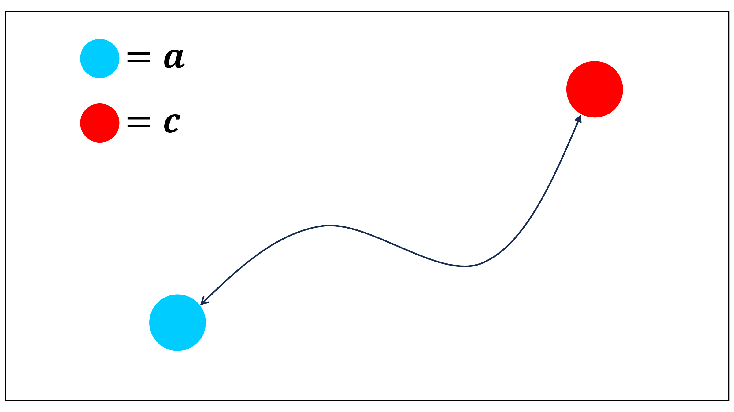
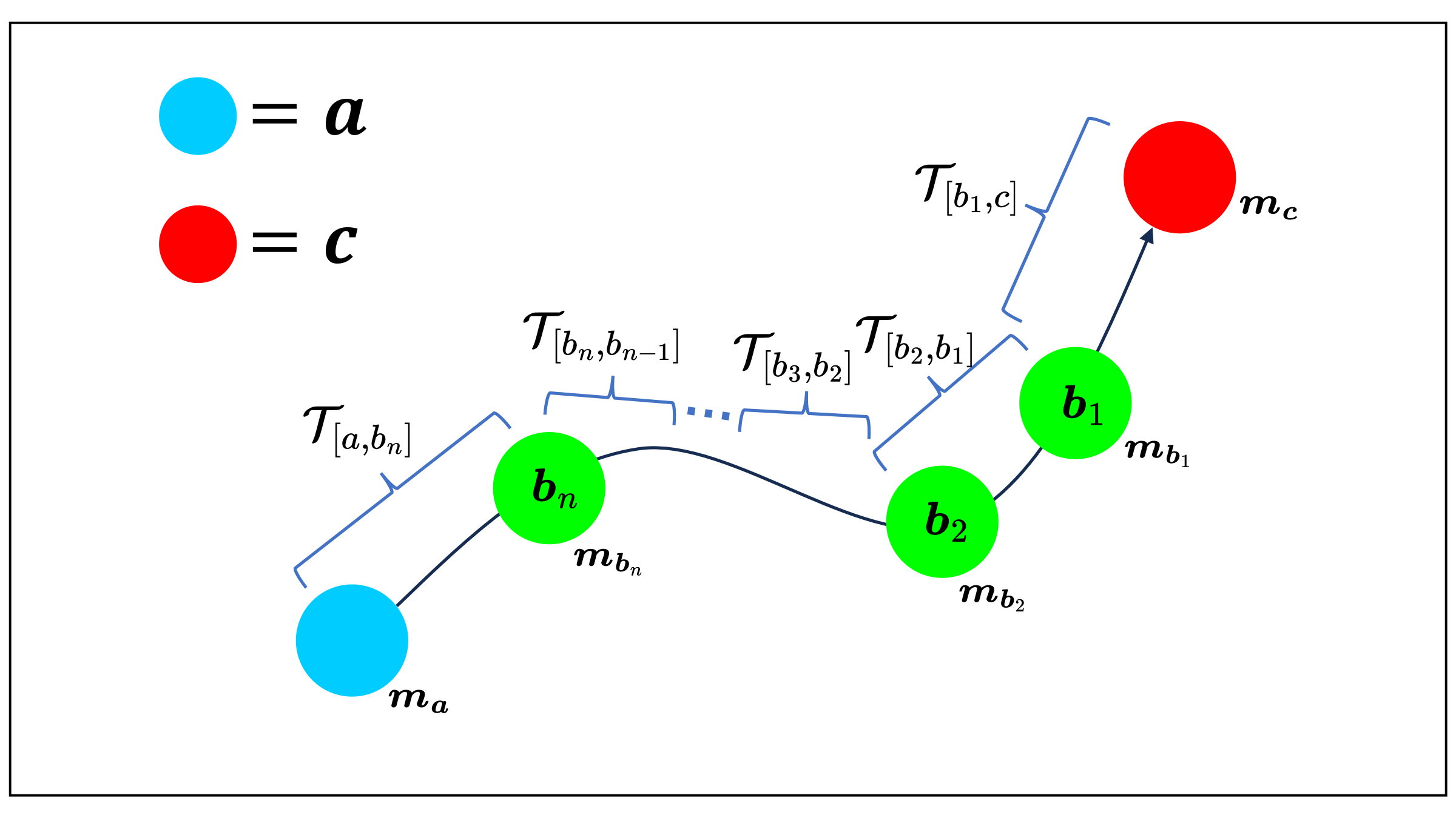
Particles inherently embody flow maps. As depicted in Figure 2, consider a particle that flows according to a spatiotemporal velocity field $\bm{u}(\bm{x},t)$ . Its trajectory, originating from time $a$ and culminating at time $c$ , characterizes both the forward map $\bm{\phi}_{[a,c]}$ and the backward map $\bm{\psi}_{[a,c]}$ . Quantities like $\mathcal{F}$ and $\mathcal{T}$ , which are determined through path integrals along a particle’s trajectory (as exemplified by the path integrals of Equation 4 for obtaining $\mathcal{F}$ and $\mathcal{T}$ ), can be calculated by conducting integrals while tracking a moving particle on the trajectory.

Next, we demonstrate that a particle flow map constitutes a perfect flow map. To establish this, we will show that a particle flow map adheres to Remarks 1 and 2.

First, consider a particle $p$ that moves according to a flow map $\bm{\phi}(\bm{X},t)$ , starting from point $\bm{X}$ at time $0$ and ending at point $\bm{x}$ at time $t$ . If we reverse this process, allowing the particle to move from $\bm{x}$ at time $t$ using the backward flow map $\bm{\psi}(\bm{x},t)$ , the particle will follow precisely the same trajectory in reverse order. This alignment of the start and end points ensures that a particle flow map inherently satisfies Remark 1.

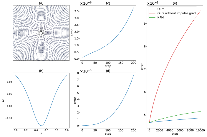
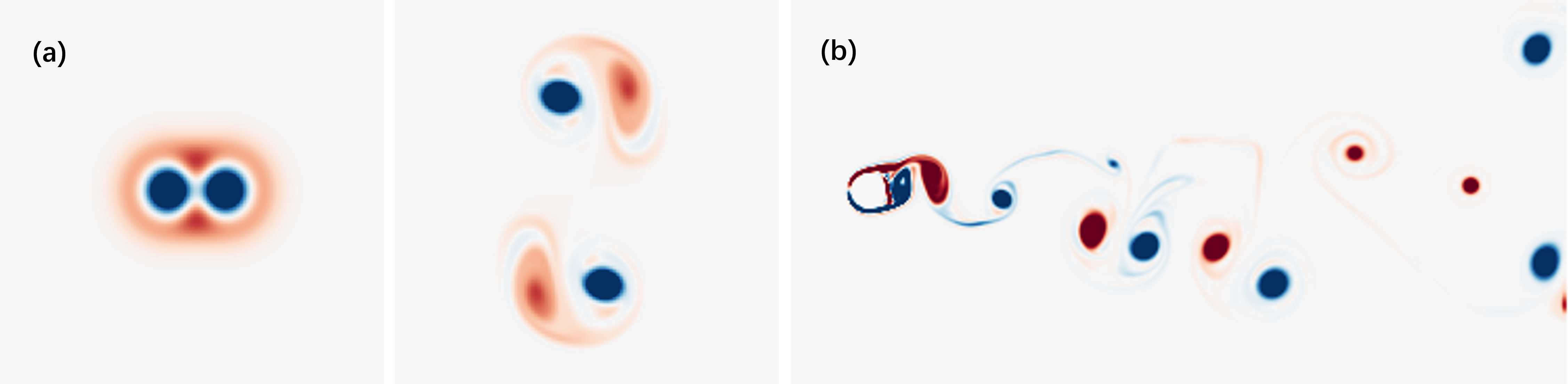
Next, we show a particle flow map also satisfies Remark 2. We carried out a numerical experiment to illustrate this: As shown in Figure 3(a) and (b), we compute $\mathcal{F}\mathcal{T}$ on particles moving in a steady velocity field defined as $\omega(r)=-0.01(1-e^{-r^{2}/0.02^{2}})/r$ and $u(x,y,r)=\omega(r)\begin{bmatrix}-y\\ x\end{bmatrix}$ where $x$ and $y$ are point locations and $r$ is the distance from point to rotation center at $(0.5,0.5)$ . As in Figure 3(c), we observed that $\mathcal{F}\mathcal{T}$ closely approximates the identity, with errors on the order of $10^{-6}$ within 200 steps. These findings confirm that flow maps on particles are in alignment with Remark 2.

4.2. Forward Evolution of $\mathcal{T}$

In NFM (Deng et al., 2023), the trajectories of the forward and backward maps do not coincide. Consequently, at each step, it’s essential to backtrack the path of a ”virtual particle” and correspondingly backward evolve $\mathcal{T}$ along this path. Practically, this procedure employs the upper part of Equation 4, but with the time dimension inverted. The requirement to backward evolve $\mathcal{T}$ from the current step back to the initial step necessitates the usage of a neural buffer for recording the velocity field at each timestep, imposing significant computational and storage costs.

Given that both the forward and backward maps in the particle flow map align with the same particle trajectory, there’s no necessity to backward evolve $\mathcal{T}$ as is done in NFM. Instead, we opt for a direct forward evolution of $\mathcal{T}$ , as demonstrated in the bottom part of Equation 4.

We further conducted an experiment to demonstrate that the forward evolution of $\mathcal{T}$ on particles yields the same results as the backward evolution. We establish a steady velocity field, as depicted in Figure 3(a) and (b). Particles are placed and move within this velocity field, and both backward and forward evolution of $\mathcal{T}$ are conducted on each particle. As illustrated in Figure 3(d), these two evolutions of $\mathcal{T}$ are nearly identical, with discrepancies on the order of $10^{-5}$ within 200 steps, which aligns with the theoretical proof that these two methods of evolution are equivalent, shown in Appendix D.

4.3. Enabling Adaptivity on a Particle Flow Map

In real simulation scenarios, it is often necessary to use flow maps of varying lengths to transport different flow quantities as mentioned in (Sato et al., 2018). For example, a long-range flow map can be used to transport the fluid impulse, while a short-range flow map may be necessary for its gradients. Generally, a quantity that is more sensitive to distortions in the background flow field, such as a high-order tensor, benefits from a shorter map. Experimenting with the length scales of these flow maps can optimize their transport effectiveness in the simulation. These needs necessitate the design of an adaptivity mechanism within our particle flow map representation.

4.3.1. Adaptive Flow Map with Temporal Samples

Fortunately, the adaptivity required can be effectively achieved through a simple idea by leveraging the Lagrangian nature of particle trajectories. As illustrated in Figure 6, we can construct an adaptive particle flow map by storing samples at different time instants $[a,b_{n},...,b_{2},b_{1},c]$ , where $a<b_{n}<...<b_{2}<b_{1}<c$ , along the particle’s trajectory from start time $a$ to end time $c$ . We capture snapshots of quantities at each time sample (e.g., $\bm{m}_{b_{n}},...,\bm{m}_{b_{2}},\bm{m}_{b_{1}}$ ), and store the backward map Jacobian between each pair of adjacent time samples (e.g., $\mathcal{T}_{[b_{i},b_{i-1}]}$ is stored between samples $b_{i}$ and $b_{i-1}$ ). With these time-axis samples created for each particle flow map, we can flexibly construct flow maps of different lengths by selecting different sample points along the trajectory as the start point, while all flow maps converge at the same endpoint, which is the same endpoint as the particle’s trajectory. The backward Jacobians from the endpoint to a chosen sample point can be computed by concatenating all Jacobians along the trajectory. For instance, for a flow map starting from the sample $b_{i}$ , the backward Jacobian $\mathcal{T}_{[b_{i},c]}$ can be calculated as $\mathcal{T}_{[b_{i},b_{i-1}]}\mathcal{T}_{[b_{i-1},b_{i-2}]}...\mathcal{T}_{[b_{1},c]}$ . The default flow map $[a,c]$ is a special case with zero sample points on the trajectory.

4.3.2. A Single-Sample Case: Long-Short Flow Map

We have implemented a single-sample strategy based on the aforementioned description to enable a long-short flow map mechanism. Between $a$ and $c$ , we position one time stamp $b$ which is closer to $c$ to construct a short map near the endpoint. This arrangement naturally produces two flow maps, $[a,c]$ and $[b,c]$ , where $[a,c]$ serves as the long flow map and $[b,c]$ as the short flow map. We store two backward Jacobians: $\mathcal{T}_{[a,b]}$ and $\mathcal{T}_{[b,c]}$ . The short backward Jacobian $\mathcal{T}_{[b,c]}$ is stored between $b$ and $c$ , and the long backward Jacobian $\mathcal{T}_{[a,c]}$ can be easily computed as shown in the following equation

(11)

\mathcal{T}_{[a,c]}=\mathcal{T}_{[a,b]}\mathcal{T}_{[b,c]}.

This long-short flow map mechanism was designed to transport both the impulse and its gradient. The long flow map is used for the long-range transport of the impulse, while the short flow map addresses the gradient, which is sensitive to flow distortion. We will specify details in Section 5.2.

At each step, we update the short-range flow map by marching $\mathcal{T}_{[b,c]}$ by one step in parallel with the particle’s advection, using our custom $4^{th}$ order of Runge-Kutta (RK4) integration scheme, as detailed in Alg. 3. Subsequently, the long-range flow map is updated according to Equation 11, with the updated $\mathcal{T}_{[b,c]}$ and $\mathcal{T}_{[a,b]}$ which has been reinitialized at time $b$ . We will demonstrate the reinitialization of the flow map in Section 4.4.

4.4. Particle Flow Map Reinitialization

Owing to the distortion that occurs in the $\mathcal{T}$ when the flow map’s range becomes excessively elongated, we reinitialize the flow map at regular intervals. Specifically, for the long-range map, a reinitialization is conducted every $n^{L}$ steps, during which time $a$ is reset to time $c$ , and $\mathcal{T}_{[a,b]}$ is set to identity:

(12)

\mathcal{T}_{[a,b]}\leftarrow\bm{I}.

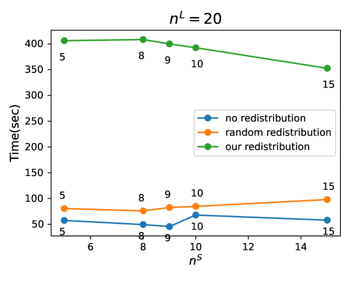
In addition, to prevent the clustering of particles over time, we will uniformly redistribute particles throughout the entire simulation domain at regular intervals of $n^{L}$ steps. Insights into the impact of this particle redistribution, as well as a comparison among different redistribution strategies, is presented in Section 7.2.

For the short-range map, a reinitialization is performed every $n^{S}$ steps, resetting time $b$ to time $c$ . Given that $\mathcal{T}_{[a,c]}$ is indirectly updated via $\mathcal{T}_{[a,b]}$ with the evolved $\mathcal{T}_{[b,c]}$ , it becomes essential to recalibrate $\mathcal{T}_{[a,b]}$ to align with the latest $\mathcal{T}_{[a,c]}$ upon each reinitialization of the short-range map, that is

(13)

\mathcal{T}_{[a,b]}\leftarrow\mathcal{T}_{[a,b]}\mathcal{T}_{[b,c]}.

Additionally, $\mathcal{T}_{[b,c]}$ is reset to the identity:

(14)

\mathcal{T}_{[b,c]}\leftarrow\bm{I}.

Moreover, particle redistribution is not performed when short-range flow map is reinitialized.

In most instances, $n^{L}$ is selected as an integer multiple of $n^{S}$ , ensuring that each reinitialization of the long-range flow map coincides with a reinitialization of the short-range flow map. However, there are situations where $n^{L}$ is not an integer multiple of $n^{S}$ . In such cases, to prevent the misalignment in the progression of the two maps, the short-range map is still reinitialized at the reinitialization points of the long-range map, even if it hasn’t reached its $n^{S}$ interval. An exploration of how these reinitialization intervals influence the process is detailed in Section 7.2.

5. Eulerian-Lagrangian Framework

Table 2. Summary of quantities stored on particles and grid.

\hlineB 3 Notation	Location	Definition
\hlineB 2.5 $\bm{x}_{p}$	particle	position of the $p$ -th particle
\hlineB 1 $\mathcal{T}_{[a,b]}$	particle	backward map Jacobian from time $b$ to $a$
\hlineB 1 $\mathcal{T}_{[b,c]}$	particle	backward map Jacobian from time $c$ to $b$
\hlineB 1 $\bm{m}_{a}$	particle	impulse on particles at time $a$
\hlineB 1 $\bm{m}_{b}$	particle	impulse on particles at time $b$
\hlineB 1 $\nabla\bm{m}_{b}$	particle	impulse gradients on particles at time $b$
\hlineB 2.5 $\bm{u}_{i}$	grid faces	velocity of the $i$ -th cell
\hlineB 1 $w_{i}$	grid faces	weights sum of the $i$ -th cell
\hlineB 3

Equipped with the design of our particle flow map, we aim to develop a hybrid Eulerian-Lagrangian framework for simulating incompressible flow. Specifically, we plan to solve the impulse-based fluid model as governed by Equation 8, utilizing the impulse flow map outlined in Equation 9. The overarching goal is to leverage particles for the accurate transport of fluid impulse and use the background grid to solve the Poisson equation and enforce incompressibility.

To construct this hybrid fluid solver, we must address three key issues: (1) The discretization of different physical quantities on particles and grids, (2) The construction of accurate flow maps for the transport of impulse, and (3) The transfer of fluid impulse from particles to the grid for the incompressibility solution. We will elaborate our numerical solutions w.r.t. these aspects as follows.

5.1. Discretization

We utilize particles to transport the fluid impulse and employ the grid for computing the divergence-free velocity field. For each particle $p$ , we store its current position $\bm{x}_{p}$ . We utilize the long-short flow map mechanism introduced in Section 4.3.2 to enable the implementation of dual-layer flow maps on each particle. In particular, we maintain two backward Jacobians, $\mathcal{T}_{[a,b]}$ and $\mathcal{T}_{[b,c]}$ , we store snapshots of the impulse values, $\bm{m}_{a}$ and $\bm{m}_{b}$ , which are sampled at times $a$ (start point of the long-range map) and $b$ (start point of the short-range map) respectively. We also store the impulse gradient $\nabla\bm{m}_{b}$ for time $b$ . On the grid side, we discretize the velocity field $\bm{u}$ on a MAC grid, with its velocity components stored on grid faces. We also store a scalar field $w_{i}$ on grid faces to specify particle-to-grid interpolation weights summation of cell $i$ . Table 2 outlines all the attributes stored on particles and the background grid. It is worth noting that a few other particle quantities, such as velocity $\bm{u}_{p}$ , endpoint impulse $\bm{m}_{c}$ , and endpoint backward Jacobian $T_{[a,c]}$ , can be calculated dynamically during the simulation. As a result, these quantities do not require dedicated storage as particle attributes.

5.2. Impulse Transport

5.2.1. Impulse Mapping

Building upon the particle flow map updated at each timestep, we first advance the fluid impulse on each particle. This process is straightforwardly executed by computing the impulse values at time $c$ , using the backward Jacobian of the long-range flow map $\mathcal{T}_{[a,c]}$ . Specifically, this can be expressed as:

(15)

\bm{m}_{c}\leftarrow\mathcal{T}_{[a,c]}^{T}\bm{m}_{a}.

Here, $\mathcal{T}_{[a,c]}$ is calculated on-the-fly by multiplying $\mathcal{T}_{[a,b]}$ and $\mathcal{T}_{[b,c]}$ .

5.2.2. Impulse Gradient Mapping

Next, we evolve the impulse gradient using our particle flow map. We map $\nabla\bm{m}_{b}$ from time $b$ to time $c$ utilizing $\mathcal{T}_{[b,c]}$ , as depicted by

(16)

\nabla\bm{m}_{c}\leftarrow\mathcal{T}_{[b,c]}^{T}\nabla\bm{m}_{b}\mathcal{T}_{[b,c]}

This equation employs the first term from the right-hand side of Equation 10, while the second term is omitted due to the overhead and difficulty of accurately calculating it. Additionally, excluding the term does not reduce the desired simulation qualities. This issue is further discussed in Section 9.

5.2.3. Impulse Particle-to-Grid Transfer

After calculating $\bm{m}_{c}$ and $\nabla\bm{m}_{c}$ , we execute a particle-to-grid transfer using values on particles to compute the impulse field $\bm{m}_{i}$ on the grid as:

(17)

\bm{m}_{i}\leftarrow\sum_{p}w_{ip}(\bm{m}_{c}^{p}+\nabla\bm{m}_{c}^{p}(\bm{x}_{i}-\bm{x}_{p}))\,/\,\sum_{p}w_{ip},

where the superscript of $\bm{m}_{c}$ and $\nabla\bm{m}_{c}$ means they are stored on particle $p$ . The impulse field $\bm{m}_{i}$ will be projected by solving Poisson equation, ultimately yielding the velocity field $\bm{u}_{i}$ on grid.

Validation Experiment

We execute an experiment to validate the efficacy of our proposed approach. Initially, we set up a velocity field as illustrated in Figure 3(a) and (b). Subsequently, particles are placed within this velocity field, and both initial velocity and velocity gradients are interpolated from the grid to the particles to establish the initial impulse and impulse gradients. The particles are then advected within the field, and both impulse and impulse gradients are evolved through the utilization of the two maps as previously described. The evolved values are then applied in a particle-to-grid process to compute the velocity field at each step. Figure 3(e) depicts the discrepancy between the analytical velocity field and the velocity field generated by our method. We also assess the outcomes when only impulse is transferred to the grid. It is evident that incorporating impulse gradients in the particle-to-grid process significantly reduces the error. In addition, we conduct this experiment using NFM, and the results of our method show a smaller discrepancy from the analytical velocity field compared to NFM, further demonstrating the efficacy of our approach.

5.3. Impulse Reinitialization

Every $n^{L}$ steps and $n^{S}$ steps, reinitialization is undertaken for long-range and short-range flow maps, respectively, as described in Section 4.4. During the reinitialization of the long-range map, since time $a$ is reset to time $c$ , particles $p$ ’s impulse $\bm{m}_{a}^{p}$ is recalibrated by interpolating the velocity field at time $c$ :

(18)

\bm{m}_{a}^{p}\leftarrow\sum_{i}w_{ip}\bm{u}_{i}.

Similarly, when the short-range flow map is reinitialized with time $b$ reset to time $c$ , particles $p$ ’s impulse gradient $\nabla\bm{m}_{b}^{p}$ is recalibrated via interpolation from the velocity field at time $c$ :

(19)

\nabla\bm{m}_{b}^{p}\leftarrow\sum_{i}\nabla w_{ip}\bm{u}_{i}.

6. Time Integration

Algorithm 1 Particle Flow Map Simulation

Initialize: $\bm{u}_{i}$ to initial velocity; $\mathcal{T}_{[a,b]}$ , $\mathcal{T}_{[b,c]}$ to $\bm{I}$

1:for

k

in total steps do

j\leftarrow k\ (\mathrm{mod}\ n^{L})

;

l\leftarrow k\ (\mathrm{mod}\ n^{S})

;

4: if

j

= 0 then

5: Uniformly distribute particles;

6: Reinitialize

\bm{m}_{a}

;

\triangleright

eq. (18)

7: Reinitialize

\mathcal{T}_{[a,b]}

\triangleright

eq. (12)

8: end if

9: if

l

= 0 then

10: Reinitialize

\nabla\bm{m}_{b}

;

\triangleright

eq. (19)

11: Reinitialize

\mathcal{T}_{[a,b]}

and

\mathcal{T}_{[b,c]}

;

\triangleright

eq. (13, 14)

12: end if

13: Compute

\Delta t

with

\bm{u}_{i}

and the CFL number;

14: Estimate midpoint velocity

\bm{u}_{i}^{\text{mid}}

;

\triangleright

Alg. 2

15: March

\bm{x}_{p}

\mathcal{T}_{[b,c]}

with

\bm{u}_{i}^{\text{mid}}

and

\Delta t

;

\triangleright

Alg. 3

16: Compute

\mathcal{T}_{[a,c]}

with

\mathcal{T}_{[a,b]}

and

\mathcal{T}_{[b,c]}

;

\triangleright

eq. (11)

17: Compute

\bm{m}_{c}

with

\bm{m}_{a}

and

\mathcal{T}_{[a,c]}

;

\triangleright

eq. (15)

18: Compute

\nabla\bm{m}_{c}

with

\nabla\bm{m}_{b}

and

\mathcal{T}_{[b,c]}

;

\triangleright

eq. (16)

19: Compute

\bm{m}_{i}

by transfering

\bm{m}_{c}

\nabla\bm{m}_{c}

to grid;

\triangleright

eq. (17)

20:

\bm{u}_{i}\leftarrow\textbf{Poisson}(\bm{m}_{i})

;

21:end for

In this section, we delineate the time integration scheme of our method, and the pseudocode of our method is outlined in Alg 1.

(1)

Reinitialize Long-range Map. Every $n^{L}$ step, we will uniformly redistribute particles throughout the entire simulation domain. Then, we reinitialize each particle’s initial long-range map impulse $\bm{m}_{a}$ by interpolating the velocity field $\bm{u}_{i}$ on grid faces, according to Equation 18. And backward map Jacobian $\mathcal{T}_{[a,b]}$ is reset to identity, outlined in Equation 12.
(2)

Reinitialize Short-range Map. Every $n^{S}$ step, each particle’s impulse gradients $\nabla\bm{m}_{b}$ are reinitialized through interpolation from the grid’s velocity field $\bm{u}_{i}$ , as depicted in Equation 19. In addition, each particle’s backward map Jacobian $\mathcal{T}_{[a,b]}$ and $\mathcal{T}_{[b,c]}$ are also reset by Equations 13 and 14.
(3)

CFL Condition. We compute $\Delta t$ with velocity field $\bm{u}_{i}$ and the CFL number.
(4)

Midpoint Method. Similar to NFM (Deng et al., 2023), we employ the second-order, midpoint method as outlined in Alg. 2 to substantially diminish the truncation error associated with temporal integration.
(5)

Advect Particles and Evolve $\mathcal{T}_{[b,c]}$ . We march $\bm{x}_{p}$ , $\mathcal{T}_{[b,c]}$ with Alg. 3, using $\bm{u}_{i}^{\text{mid}}$ and $\Delta t$ .
(6)

Compute $\mathcal{T}_{[a,c]}$ . We employ $\mathcal{T}_{[a,b]}$ and $\mathcal{T}_{[b,c]}$ to calculate $\mathcal{T}_{[a,c]}$ , according to Equation 11.
(7)

Compute $\bm{m}_{c}$ . We evolve $\bm{m}_{a}$ from time $a$ to time $c$ using long-range map to calculate $\bm{m}_{c}$ , according to Equation 15.
(8)

Compute $\nabla\bm{m}_{c}$ . We evolve $\nabla\bm{m}_{b}$ from time $b$ to time $c$ using short-range map to calculate impulse gradients $\nabla\bm{m}_{c}$ , according to Equation 16.
(9)

Particle-to-grid. We transfer impulse $\bm{m}_{c}$ and impulse gradients $\nabla\bm{m}_{c}$ from particles to grid faces, resulting in impulse field $\bm{m}_{i}$ on grid, according to Equation 17.
(10)

Poisson Solving. We obtain velocity field $\bm{u}_{i}$ on the grid from impulse field $\bm{m}_{i}$ by solving Poisson equation.

7. Validation

The goal of this section is to validate the effectiveness of our proposed method. We will first introduce a variation of PFM, which will be used for comparison. Then, we will compare PFM with five methods to validate its effectiveness. Next, we will conduct an ablation study to validate some steps of our method.

7.1. Comparison to Other Approaches

In this section, we assess the effectiveness of our method against established benchmarks, including methods of CF (Nabizadeh et al., 2022), CF+BiMocq (Nabizadeh et al., 2022; Qu et al., 2019), NFM (Deng et al., 2023), APIC (Jiang et al., 2015), and an impulse-modified APIC (IM APIC) as we specified below. Our primary focus lies in comparing our method with these techniques regarding vortex preservation capabilities, energy conservation, visual intricacy, and the computational time and memory costs involved in the simulations.

Impulse-modified APIC

To showcase that the particle flow map mechanism plays an essential role, we implemented an impulse-modified APIC solver to conduct ablation tests. By configuring both $n^{L}$ and $n^{S}$ to 1, effectively causing the long-range map and short-range map to be reinitialized at every step, PFM transitions into a methodology closely resembling APIC (Jiang et al., 2015), with the primary distinction being the substitution of impulse for velocity. We refer to this variation as impulse-modified APIC. In this approach, particles at each step interpolate the grid’s velocity field to acquire impulse and impulse gradients. Then, the backward map Jacobian $\mathcal{T}$ is calculated similarly to the approach in PFM. These elements are utilized to evolve the impulse and impulse gradients by a single step during the particle advection process. Subsequently, the evolved values are conveyed to the grid via a particle-to-grid process mirroring PFM’s. An evaluative comparison between impulse-modified APIC and PFM is detailed in the following experiments.

Table 3. Simulation world time (frames

\times

timestep) of 2D leapfrogging vortices from the initial state to the end state. The observation reveals that APIC, impulse-modified APIC, CF, and CF+BiMocq are unable to maintain the vortices over an extended period. On the other hand, the NFM exhibits improved performance, yet it remains less effective compared to the PFM.

\hlineB 3 Method	Time (sec)
\hlineB 2.5 APIC	7.9
\hlineB 1 IM APIC	92.0
\hlineB 1 CF	50.1
\hlineB 1 CF+BiMocq	45.0
\hlineB 1 NFM	234.0
\hlineB 1 Ours	408.5
\hlineB 1 Ours+Hessian	317.5
\hlineB 3

2D Analysis: Leapfrogging Vortices

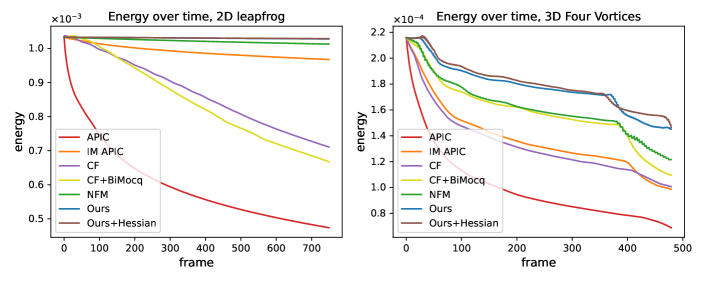
We establish the classic 2D leapfrogging vortex rings experiment. Initially, two negative and two positive vortices are placed on the left side of the domain. These vortices then move rightward and eventually return to their starting positions after colliding with the boundary. In an energy-conserving scenario, this cycle could continue indefinitely. However, in practical simulations, the vortices either merge into a single negative and a single positive vortex, or the two pairs become asymmetric along the $y$ -axis. Both outcomes indicate numerical diffusion in the simulation. We timed the duration from the initial configuration to one of these end states, and the performance of various methods is summarized in Table 3. The results reveal that the APIC method maintains the vortices for only a brief period before they dissipate, whereas impulse-modified APIC, CF, and CF+BiMocq perform slightly better than APIC. The NFM method outperforms them but is still surpassed by PFM. This is consistent with the energy variation results presented in Figure 12, where PFM excels in energy preservation over the other methods.

Interestingly, although impulse-modified APIC also utilizes evolved impulse and impulse gradients on particles to reconstruct the velocity field, its effectiveness in maintaining vorticity is significantly inferior to that of PFM. This indicates that merely using impulse and impulse gradients is insufficient. For optimal vorticity retention, it is crucial to evolve these elements on particles using a flow map with adequate range, thereby enhancing numerical accuracy.

3D Analysis: Leapfrogging Vortices

As illustrated in Figure 13, we experiment with 3D leapfrogging vortex rings. Analogous to the 2D scenario, two rings in this experiment will perpetually leapfrog around each other in a conservative setting. In our findings, APIC, impulse-modified APIC, CF and CF+BiMocq manage to keep the two rings separate only up to the $3^{\text{rd}}$ leap. And both NFM and PFM successfully sustain to the $5^{\text{th}}$ leap.

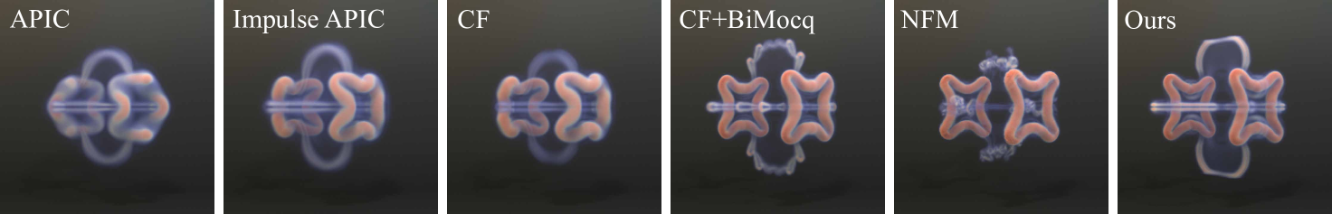
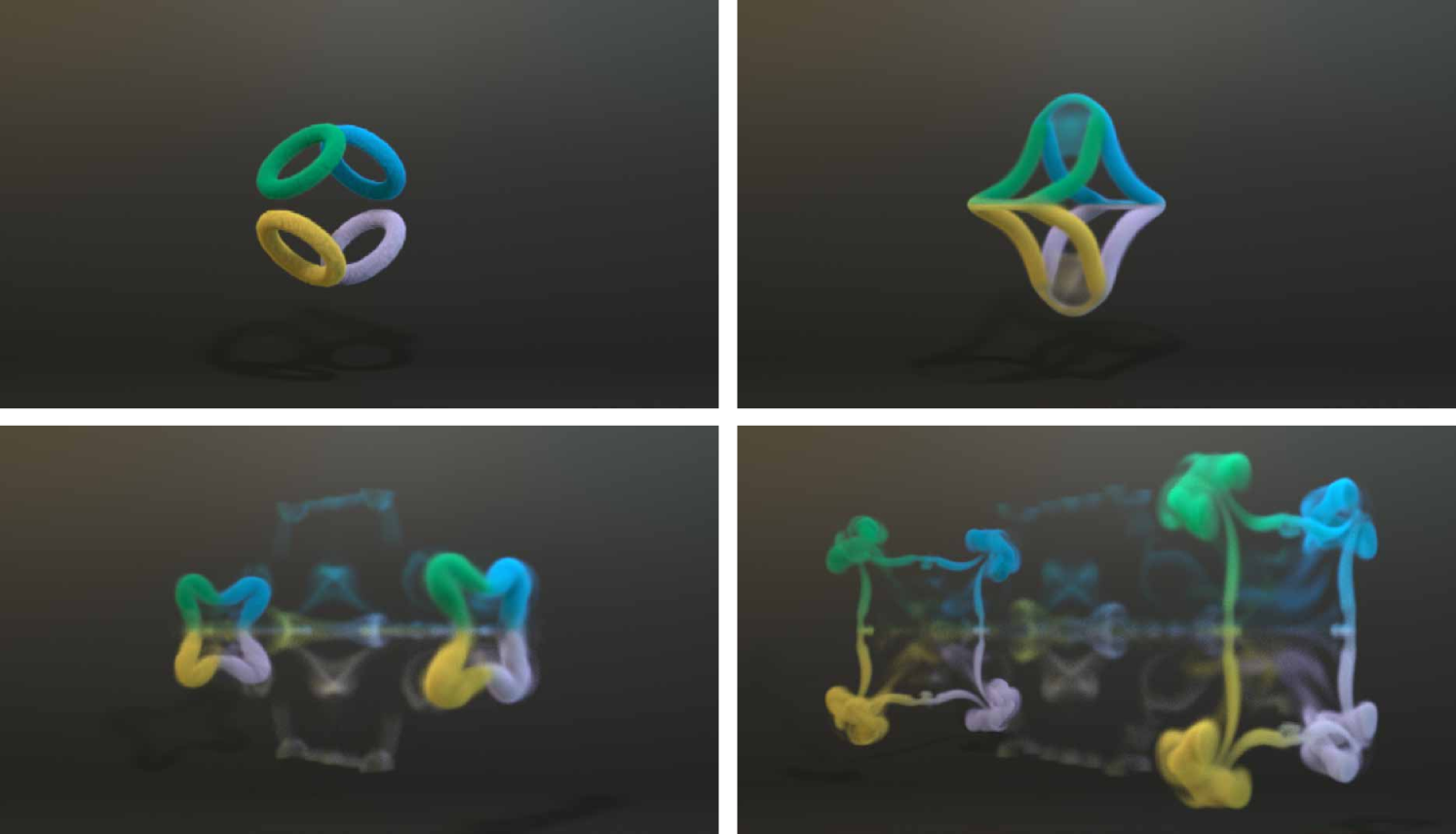
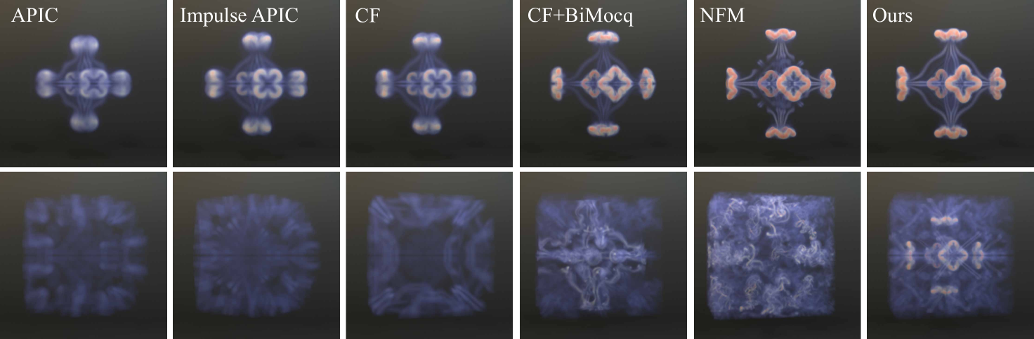
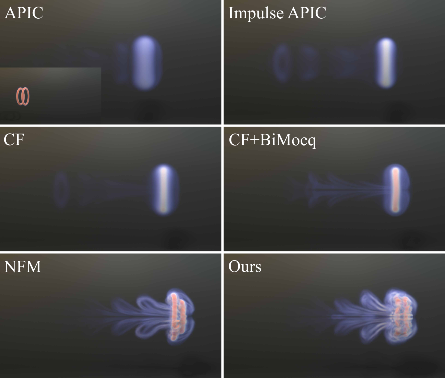
3D Analysis: Four Vortices Collision

As depicted in Figure 10, we execute an experiment involving the collision of four vortices, during which the vortices merge and subsequently divide into two star-shaped vortices that drift in opposite directions until they encounter the boundary. We compare the simulation results of PFM to the other methods, as shown in Figure 14. The results reveal that all six methods can generate the twin star-shaped vortices. However, post-collision, APIC, impulse-modified APIC, and CF struggle to maintain vorticity, leading to dissipative, slower-moving vortices. In contrast, CF+BiMocq, NFM, and PFM effectively preserve vorticity. This observation is consistent with the time-varying energy analysis presented in Figure 12, where APIC, impulse-modified APIC, and CF exhibit rapid energy loss, whereas CF+BiMocq, NFM and PFM demonstrate superior energy conservation, with PFM outperforming CF+BiMocq and NFM in this regard.

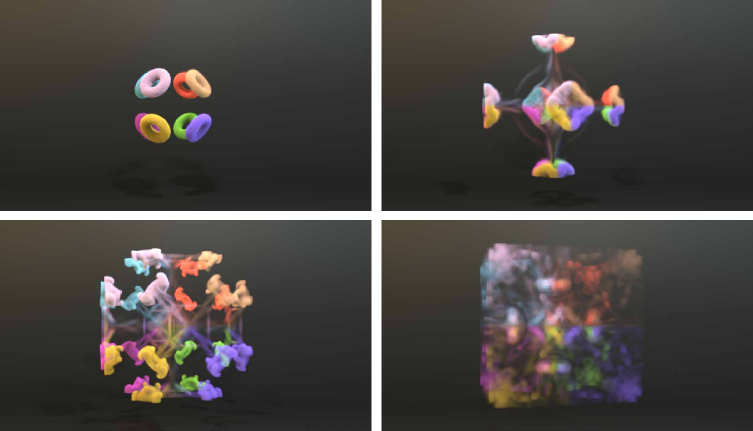
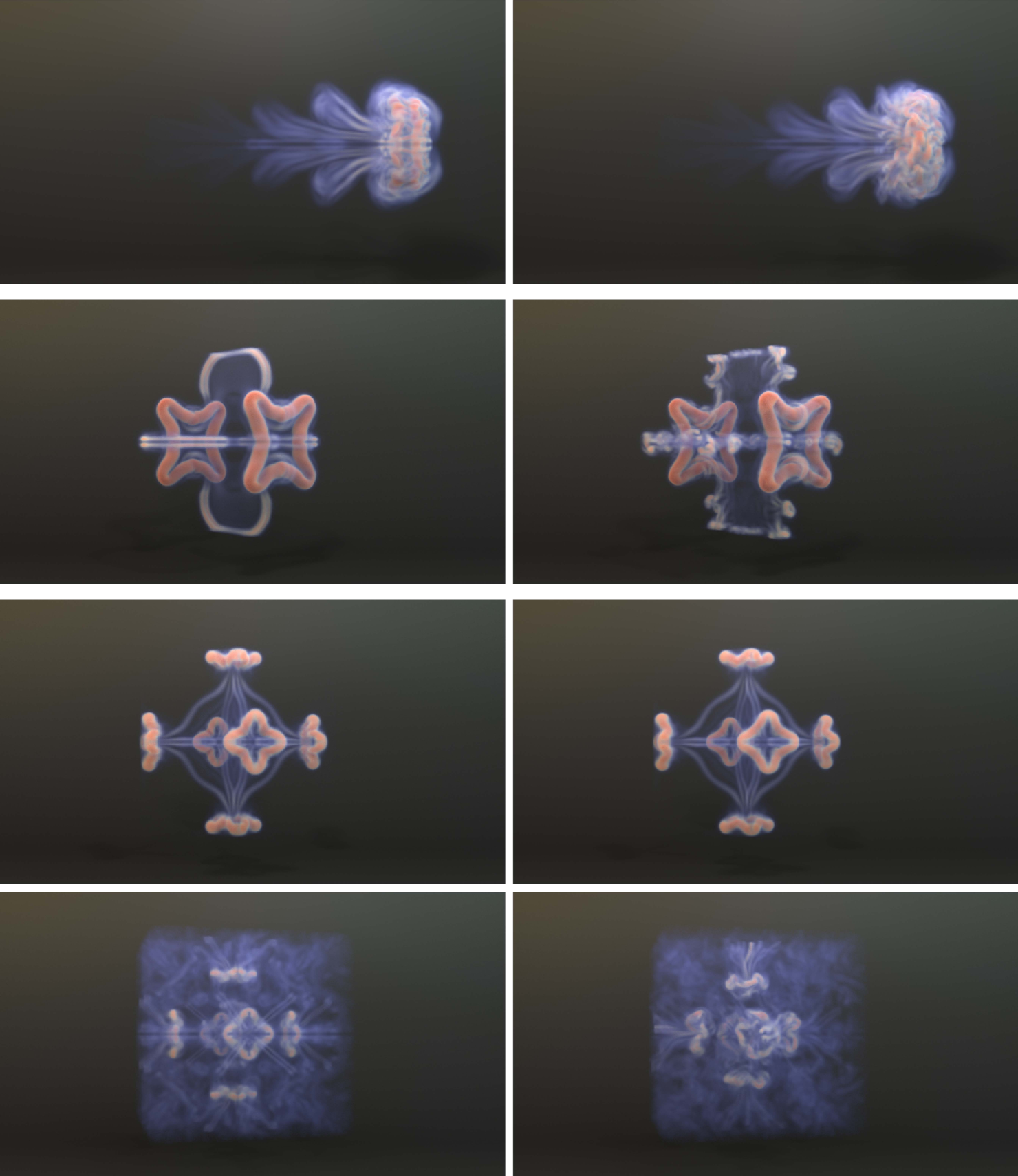
3D Analysis: Eight Vortices Collision

As illustrated in Figure 10, we undertake an experiment involving the collision of eight vortices. The amalgamation of these vortices forms six star-shaped vortices, which proceed along the positive and negative axes of three orthogonal dimensions. Upon impact with the cube-shaped boundary, the vortices disperse into several vortex tubes, tracing the boundary surface before eventually merging to reconstruct six distinct vortices. As shown in Figure 11, APIC, impulse-modified APIC, and CF exhibit excessive dissipation, failing not only to preserve the vortical structures but also to regenerate the six vortices. While CF+BiMocq and NFM manages to maintain the tubular formations, it falls short in preserving the overall symmetry of the system. In contrast, PFM preserves the entire system’s symmetry and effectively reconstructs the six-vortex formation.

Table 4. Average simulation time and maximum GPU memory cost of our 2D and 3D simulation examples.

\hlineB 2 Name	Method	Time (sec / step)	GPU Mem. (GB)
\hlineB 1.5 2D Leapfrog	APIC	0.24	1.21
2D Leapfrog	IM APIC	0.25	1.41
2D Leapfrog	NFM	23.11	2.00
2D Leapfrog	Ours	0.47	1.41
\hlineB 1 3D Leapfrog	APIC	4.92	3.51
3D Leapfrog	IM APIC	4.69	7.91
3D Leapfrog	NFM	52.05	13.33
3D Leapfrog	Ours	4.75	8.21
\hlineB 1 3D Four Vort	APIC	4.60	3.51
3D Four Vort	IM APIC	4.26	7.91
3D Four Vort	NFM	50.71	13.34
3D Four Vort	Ours	4.20	8.21
\hlineB 1 3D Eight Vort	APIC	2.04	2.31
3D Eight Vort	IM APIC	1.82	4.41
3D Eight Vort	NFM	47.98	7.91
3D Eight Vort	Ours	1.95	4.61
\hlineB 2

Time and Memory Cost Analysis

As depicted in Table 4, PFM significantly outperforms NFM in terms of execution speed, delivering results comparable to or surpassing those achieved by NFM. Specifically, PFM is 49.1, 10.9, 12.0, and 24.6 times faster than NFM in scenarios involving 2D leapfrogging vortices, 3D leapfrogging vortices, 3D four vortices collision, and 3D eight vortices collision, respectively. This considerable increase in speed primarily stems from eliminating both the backtrack substeps and the neural buffer training process present in NFM. Moreover, by obviating the need for a neural buffer, PFM also realizes substantial memory savings, registering reductions of 29.5%, 38.4%, 38.4%, and 41.7% in memory usage compared to NFM for these respective scenarios. Compared to APIC and impulse-modified APIC, PFM maintains a similar execution time and memory footprint, yet it significantly enhances the simulation outcomes for these examples, as previously mentioned.

7.2. Ablation Study

Redistribute Particles

We conduct a 2D leapfrogging vortices analysis using three different particle redistribution strategies: uniform particle redistribution, random particle redistribution, and no particle redistribution. These approaches are examined under conditions where ( $n^{L}$ , $n^{S}$ ) assumes values of (20, 5), (20, 8), (20, 9), (20, 10), and (20, 15). The simulation world time from the initial state to the end state of the leapfrogging vortices, utilizing the three mentioned strategies, is illustrated in Figure 17. The results indicate that both the no redistribution and random redistribution methods fall short of achieving satisfactory results, with random redistribution slightly outperforming the former. However, it is the uniform particle redistribution that delivers the most efficient performance, an approach that is notably employed by PFM.

Reinitialization Steps

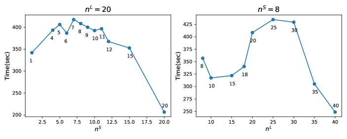
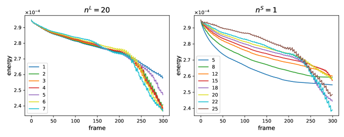
We examine the impact of reinitialization intervals $n^{L}$ and $n^{S}$ by conducting both 2D and 3D leapfrogging vortices experiments. Specifically, for the 2D scenario, we set $n^{S}$ to values of 1, 4, 5, 6, 7, 8, 9, 10, 11, 12, 15, and 20 when $n^{L}$ is fixed at 20, and we alter $n^{L}$ to 8, 10, 15, 18, 20, 25, 30, 35, and 40 when $n^{S}$ is fixed at 8. For 3D scenario, we set $n^{S}$ to values of 1, 2, 3, 4, 5, 6 and 7 when $n^{L}$ is fixed at 20, and we alter $n^{L}$ to 5, 8, 12, 15, 18, 20, 22 and 25 when $n^{S}$ is fixed at 1. The outcomes are depicted in Figure 19 and 20 for 2D and 3D experiments, respectively. The results reveal that for a constant $n^{L}$ , a smaller $n^{S}$ typically yields better results. However, as $n^{S}$ approaches the value of $n^{L}$ , the efficiency of PFM diminishes rapidly. This confirms the importance of using both short-range and long-range maps in PFM instead of two flow maps of identical lengths. Conversely, when $n^{S}$ is held constant, both excessively large and small values of $n^{L}$ lead to suboptimal performance.

Evolution of Smoke Density Gradients

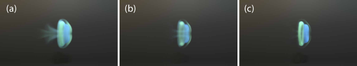
In our method, we employ a particle-to-grid strategy that not only facilitates the transport of vector quantities such as impulse, transferring both the quantity itself and its evolved gradients to the grid, but also extends this methodology to the transport of scalar quantities, like smoke density $\rho_{s}$ . This section highlights the importance of accurately evolving $\nabla\rho_{s}$ with the flow map and effectively transferring it from the particles to the grid, especially in smoke advection. In our approach, we store both the smoke density $\rho_{s}$ and its gradients $\nabla\rho_{s}$ on particles, with the gradients evolving using the flow map. Subsequently, we employ a strategy akin to that used for impulse to transfer these values to the grid. We show in Figure 18 that not transferring $\nabla\rho_{s}$ to the grid or not evolving $\nabla\rho_{s}$ will cause smoothing behavior in smoke simulation. The first subfigure shows the smoke advected without $\nabla\rho_{s}$ , and the smoke gets blurred quickly. The middle subfigure shows that if we keep $\nabla\rho_{s}$ for reinitialization without evolving it, smoke also gets blurred (but slightly better). Only by evolving $\nabla\rho_{s}$ and transferring both $\rho_{s}$ and $\nabla\rho_{s}$ can we obtain the optimal result.

8. Examples

In this section, we present various intricate simulation examples to demonstrate the efficacy of our PFM simulator. A comprehensive list of these examples and their respective configurations is available in Table 5. It is assumed that the shortest edge of the simulation domain is of unit length. We refer readers to our supplemented video for detailed simulation results. All simulations were performed on workstations equipped with an AMD Ryzen Threadripper 5990X and an NVIDIA RTX 3080/A6000.

8.1. Vortical Flow

Taylor Vortex

We adapt the setting from (McKenzie, 2007) where the simulation domain is $[-\pi,\pi]$ and two Taylor vortices separated by $0.8$ . We show the separation process in Figure 22.

Leapfrogging Vortices (2D)

Table 3 shows our 2D leapfrog experiment where we position four point vortices with equal magnitudes of 0.005 at $x$ = 0.0625 and $y$ values of 0.26, 0.38, 0.62, and 0.74, with the upper two negative and the lower two positive. These vortices are modeled using a mollified Biot-Savart kernel with a support of 0.02. In the experiment, our method accurately maintains vortex structure for 408.5 seconds.

Leapfrogging Vortices (3D)

In Figure 16, the initial setup involves two vortex rings aligned parallelly, positioned at $x$ = 0.16 and 0.29125. These rings have a major radius of 0.21 and a minor radius (the mollification support of the vortices) of 0.0168. Our approach maintains separation of the vortex rings beyond the $5^{\text{th}}$ leap.

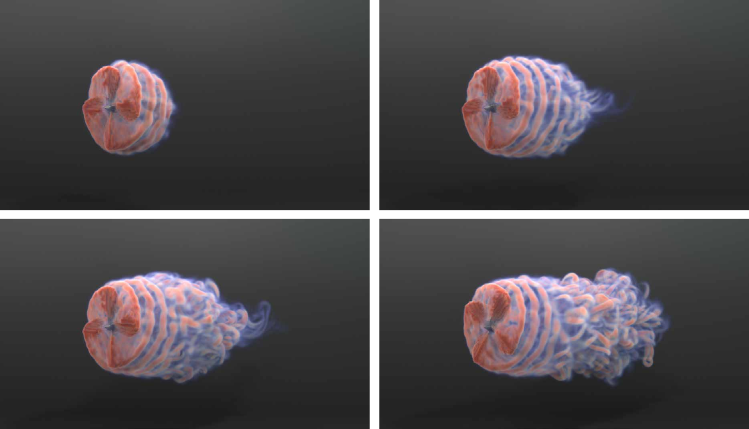
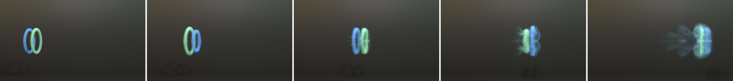
Oblique Vortex Collision

In Figure 8, we detail an experiment with two perpendicular vortex rings, offset by 0.3 units along the $x$ -axis, each having a major radius of 0.13 and a minor radius of 0.02.

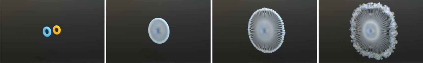
Headon Vortex Collision

Figure 15 shows an experiment with two opposing vortex rings, separated by 0.3 units on the $x$ -axis, each with a major radius of 0.065 and a minor radius of 0.016. When these rings collide, they form a single ring that elongates in the $yz$ -plane and contracts along the $x$ -axis, leading to destabilization and fragmentation into secondary vortices (Lim and Nickels, 1992).

Trefoil Knot

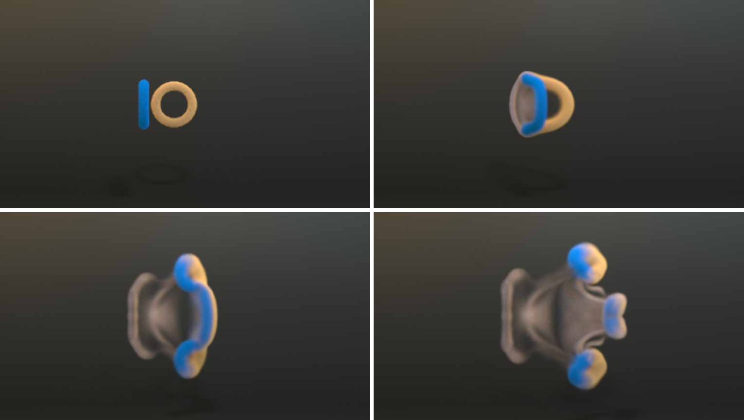
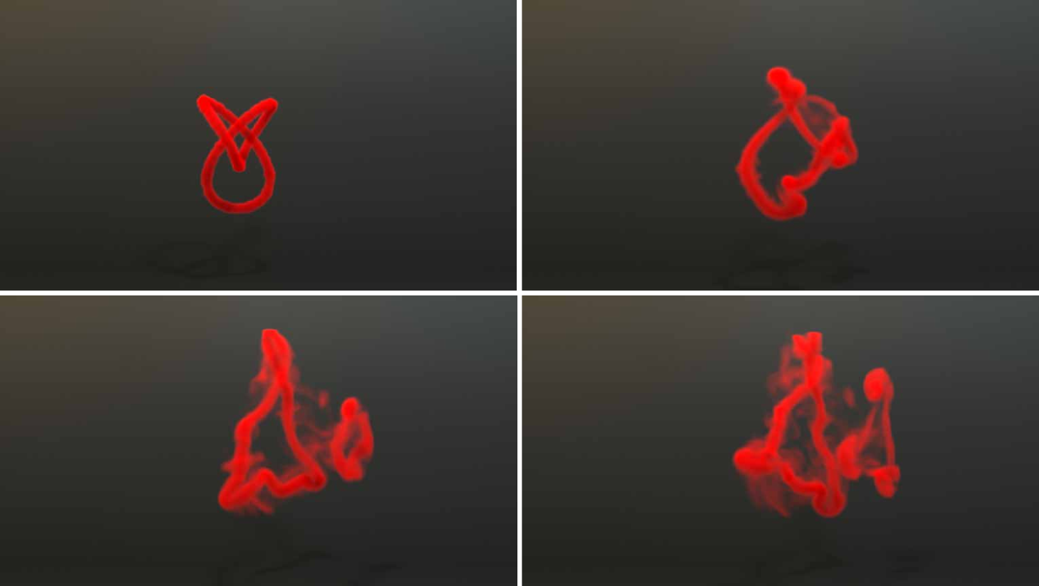
Figure 8 replicates the trefoil knot, using an initialization file from Nabizadeh et al. (2022), based on Kleckner and Irvine (2013). Our simulation result matches the experiments.

Four Vortices Collision

Figure 10 depicts an experiment based on Matsuzawa et al. (2022) where four vortex rings, arranged in a square pattern, collide in the $yz$ -plane. These rings, each with a major radius of 0.15 and a minor radius of 0.024 merge into two four-pointed star-shaped vortices until colliding with the boundaries. We compare our result with previous methods in Figure 14.

Eight Vortices Collision

Figure 10, based on Matsuzawa et al. (2022), shows an experiment with eight vortices forming a regular octahedron, each angled at 35.26° relative to the $z$ -axis. These rings, with major radius of 0.08 and minor radius of 0.024, collide and reconnect into six rings within a cubic boundary. Figure 11 shows our method uniquely recreating this dynamic.

8.2. Solid Boundaries

We employ a triangle mesh for solid-driven flow applications, either static or animated by a preset skeleton. The forward difference between two consecutive timesteps determines the velocity at each mesh vertex. We adopt an interpolation method, as described in (Robinson-Mosher et al., 2008), to transfer velocity from mesh vertices to a grid. The weight of this transfer is based on the intersection area between the grid cell and the triangle patch. This velocity is then used as a solid boundary condition to drive the fluid simulation.

Karman Vortex Street

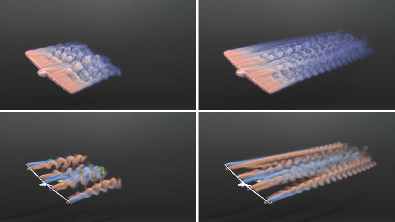
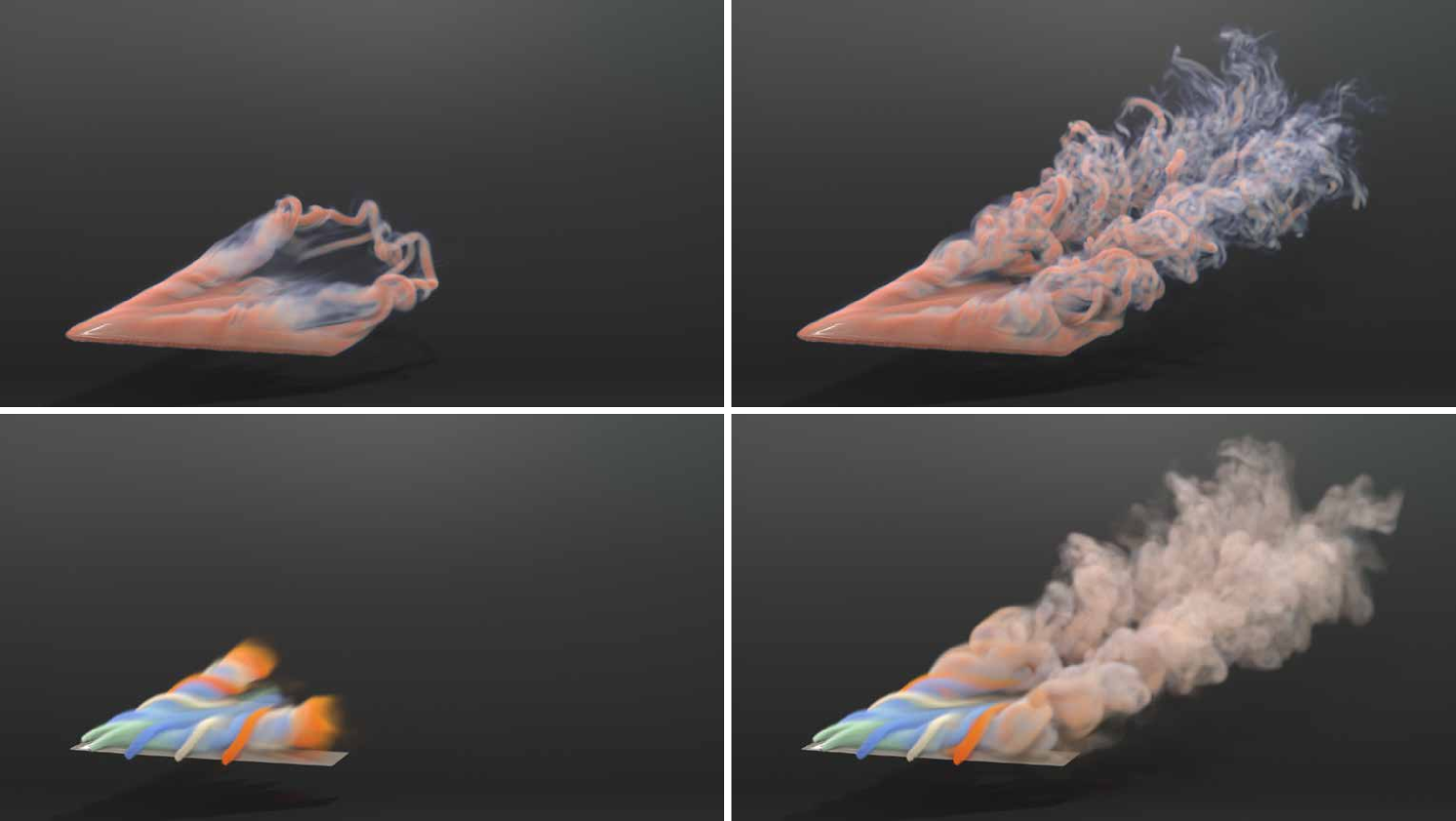
In Figure 22, we place a cylinder at [0.2, 0.5] with the radius of 0.05. Due to lack of viscosity, incoming flow creates more turbulent vortices, as shown in (Nabizadeh et al., 2022).

Lifting Airplane

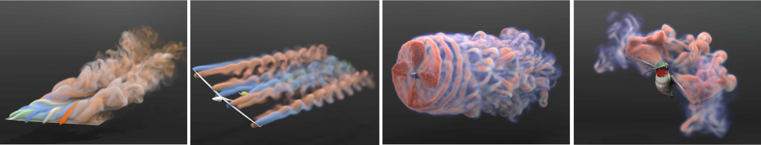
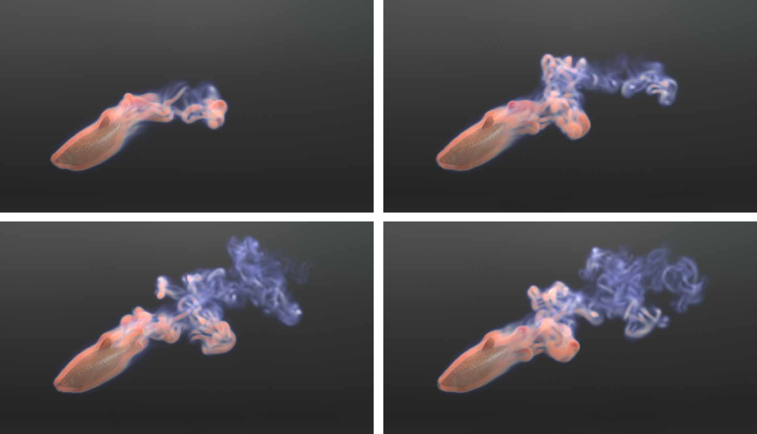
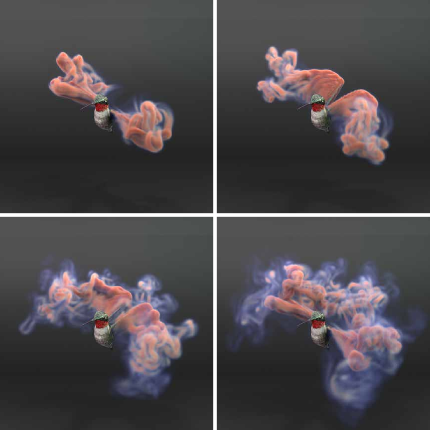
In Figures 24 and 24, we showcase planes with different lifting angles facing incoming flow from the front boundary. Both delta wing and flat wing configurations are depicted. The trajectories observed in our smoke visualization model closely mimic real-world airplane condensation trails.

Flapping Bird, Swimming Fish, and Rotating Propeller

Figure 21, 5 and 5 illustrate our method coupling with the skeleton driven meshes. Skeletons are built in Blender in each example and set with periodic movements such as continuous rotations. Bezier interpolations between keyframes are performed to ensure smoothness.

Table 5. The catalog of all our 2D and 3D simulation examples.

n^{L}

and

n^{S}

are the reinitialization steps of long-range and short-range maps, respectively, and #Particles is the particle count per cell at reinitialization step.

\hlineB 3 Name	Figure/Table	Resolution	CFL	$n^{L}$	$n^{S}$	#Particles
\hlineB 2.5 2D Leapfrog	Table 3	1024 $\times$ 256	1.0	20	8	16
\hlineB 2 2D Taylor Vortex	Figure 22 (a)	128 $\times$ 128	1.0	20	8	16
\hlineB 2 2D Karman Vortex	Figure 22 (b)	512 $\times$ 256	0.5	20	8	16
\hlineB 2 3D Leapfrog	Figure 16	256 $\times$ 128 $\times$ 128	0.5	20	1	8
\hlineB 2 3D Oblique	Figure 8	128 $\times$ 128 $\times$ 128	0.5	12	4	8
\hlineB 2 3D Headon	Figure 15	128 $\times$ 256 $\times$ 256	0.5	12	4	8
\hlineB 2 3D Trefoil	Figure 8	128 $\times$ 128 $\times$ 128	0.5	12	1	8
\hlineB 2 3D Four Vortices	Figure 10	128 $\times$ 128 $\times$ 256	0.5	12	4	8
\hlineB 2 3D Eight Vortices	Figure 10	128 $\times$ 128 $\times$ 128	0.5	12	4	8
\hlineB 2 Flat Wing	Figure 24	384 $\times$ 128 $\times$ 128	0.5	12	4	8
\hlineB 2 Delta Wing	Figure 24	384 $\times$ 128 $\times$ 128	0.5	12	4	8
\hlineB 2 Flapping Bird	Figure 21	128 $\times$ 128 $\times$ 128	0.5	12	4	8
\hlineB 2 Swimming Fish	Figure 5	256 $\times$ 128 $\times$ 128	0.5	12	4	8
\hlineB 2 Rotating Propeller	Figure 5	256 $\times$ 128 $\times$ 128	0.5	12	4	8
\hlineB 3

9. Discussion and Conclusion

In this paper, we present a particle flow map method (PFM) that achieves state-of-the-art advection fidelity and simulation accuracy in terms of energy conservation, vorticity preservation, and visual complexity, through its novel bridging of impulse fluid mechanics, long-range flow map, and hybrid Eulerian-Lagrangian simulation. Compared to the accurate but expensive NFM method, our PFM method drastically reduces the computational cost without sacrificing the physical fidelity, as it leverages the mathematical and numerical insight that a set of forward-evolving equations can be derived and naturally solved on particles to replace the costly backtracing procedure. To realize this idea to its full potential, we carefully devise a two-scale flow map representation along with a novel particle-to-grid transfer scheme to devise a hybrid solver whose accuracy and versatility are thoroughly verified through a set of challenging numerical experiments, including leapfrogging vortices, vortex tube reconnections, and turbulent flows.

Connection to NFM

The goal for both PFM and NFM is to accurately compute impulse $\bm{m}$ on the grid, but they present two different numerical perspectives: NFM traces “virtual particles” whose final positions coincide with the grid points, but their initial positions are inside grid cells. Hence, a grid-to-particle interpolation scheme is required at the initial time. PFM maintains forward simulating particles whose final positions are inside cells, but their initial values are known from (re)initialization. Hence, a particle-to-grid transfer scheme is required at the final time. As a result, both perspectives require exactly one potentially lossy communication between particles and grids for each simulation step. To this end, NFM uses a naive linear interpolation scheme and compensates for the interpolation error with BFECC (Kim et al., 2006). PFM, on the other hand, devises an advanced particle-to-grid transfer scheme that largely reduces the error. Thus, for accuracy, both methods offer comparable levels of performance, which are validated in our experiments. However, from the efficiency standpoint, PFM is by far more desirable due to the elimination of the costly backtracing process, as it can be up to $49\times$ faster and $41\%$ more compact than NFM.

Connection to Hybrid Eulerian-Lagrangian Methods

Our PFM method presents itself as a new type of hybrid Eulerian-Lagrangian method, which is in line with PIC (Harlow, 1962), APIC (Jiang et al., 2015), and similar methods, but one with significantly improved ability to preserve the vortical structure, which is enabled by its innovative exploitation of the particles’ roles not only as samples of physical fields but as samples of high-quality and adaptive-range flow maps. With this new perspective, we devise novel mathematical formulations to endow particles with the crucial ability to evolve backward map Jacobian $\mathcal{T}$ in a forward-simulating manner, which allows our hybrid framework to be readily bridged with the highly effective impulse-based fluid paradigm. Not only is combining Lagrangian particles with a flow map physically inspired and computationally efficient, but it also naturally empowers the development of our length-adaptive mechanism, which is shown to be key to successful simulation, as verified in our ablation tests. Inspired by the conservative transfer schemes proposed by APIC (Jiang et al., 2015) and Taylor-PIC (Nakamura et al., 2023), our method conservatively transfers $\bm{m}$ by leveraging its evolved gradients $\nabla\bm{m}$ , and our scheme can be seen as a generalization of APIC as it allows $\nabla\bm{m}$ to be accurately evolved using adaptive-length flow maps rather than single-step ones. In our comparison tests with APIC, we showcase that such an improved accuracy for $\nabla\bm{m}$ contributes to the simulation accuracy.

Further Ablation Tests on Hessian

We excluded the Hessian term in Equation 10 in our proposed numerical implementation in Section 5.2. In this section, we provide further ablation tests to evaluate the efficacy of Hessian in enhancing numerical accuracy. We calculated backward map Hessian $\nabla\mathcal{T}_{[b,c]}^{p}$ for each particle $p$ by aggregating backward map Jacobian $\mathcal{T}_{[b,c]}^{k}$ of its neighboring particles, weighted by $\nabla w_{pk}$ , where $k$ is the index of the neighboring particle. We then included $(\nabla\mathcal{T}_{[b,c]}^{p})^{T}\bm{m}_{b}$ to the right-hand side of Equation 16 to align it with Equation 10. Then, we conduct validation experiments with the same setup as detailed in Section 7.1 and show the results in Table 3 and Figure 25 for 2D and 3D leapfrogging vortices, four vortices collision, and eight vortices collision. Additionally, the time-varying energy for the 2D leapfrogging vortices and four vortices collision is depicted in Figure 12. From 2D/3D leapfrog experiments, we observed no significant improvement in preserving vortical structures compared to our proposed scheme. Similarly, the formula incorporating the Hessian term does not preserve symmetry structures as effectively in four/eight vortices collision experiments as our scheme does. We conjecture that this discrepancy in ability is due to potential inaccuracies in the backward map Hessian when directly calculated from particles, which leads to errors in mapping impulse gradients through flow maps. Furthermore, from a theoretical perspective, we observe that our method corresponds to a specific case of transferring $\mathcal{T}$ from particles to the grid. We demonstrate that using only the first term on the right-hand side of Equation 10 is equivalent to this transfer in a PIC (Harlow, 1962) manner, as detailed in Appendix F. Conversely, including the Hessian term modifies the transfer method from PIC to an APIC (Jiang et al., 2015) manner. Consequently, inspired by APIC’s enhancements over PIC, we anticipate uncovering additional numerical benefits by incorporating the Hessian term towards a higher-order PFM in our future exploration.

Uniform Particle Redistribution

Uniform particle redistribution (or otherwise terms as remeshing or regridding) has been a widely used practice to address the particle distortion problem in the Vortex-In-Cell (VIC) literature (Koumoutsakos et al., 2008). As consolidated in Figure 17, a uniform sampling strategy is necessary to reduce the interpolation error for the impulse grid-to-particle transfer. We conjure the reason to be the fact that we are transferring $\mathcal{T}$ from particles to the grid, as shown in the previous discussion, and when reinitialization happens, uniform redistributing particles gives a more structured reconstruction of its current space.

Limitations & Future Works

Our method is currently subject to a few limitations. First, it currently considers Euler’s equation for inviscid fluid flows, and the incorporation of viscosity and diverse external forces remains an open problem for our flow map-based framework. Secondly, handling interfacial phenomena still proves challenging for our impulse-based formulation as it introduces additional terms in the Poisson equation which brings about considerable numerical instability. Solving these technical challenges will allow free-surface liquids to be simulated which unlocks a new range of vortical phenomena like toroidal bubbles. Finally, we currently employ kinematic coupling for handling solid-fluid interactions, and the development of dynamic two-way coupling schemes in the PFM framework would be an exciting future challenge.

Acknowledgements

We express our gratitude to the anonymous reviewers for their insightful feedback. We especially appreciate Zhiqi Li for his insights on the connection between the Hessian term and the transfer of the backward map Jacobian. We also thank Jinyuan Liu and Taiyuan Zhang for their insightful discussion. Georgia Tech authors acknowledge NSF IIS #2313075, ECCS #2318814, CAREER #2420319, IIS #2106733, OISE #2153560, and CNS #1919647 for funding support. We credit the Houdini education license for video animations.

References

(1)
Ando and Tsuruno (2011) Ryoichi Ando and Reiji Tsuruno. 2011. A particle-based method for preserving fluid sheets. In Proceedings of the 2011 ACM SIGGRAPH/Eurographics symposium on computer animation. 7–16.
Brackbill and Ruppel (1986) Jeremiah U Brackbill and Hans M Ruppel. 1986. FLIP: A method for adaptively zoned, particle-in-cell calculations of fluid flows in two dimensions. Journal of Computational physics 65, 2 (1986), 314–343.
Buttke (1992) TF Buttke. 1992. Lagrangian numerical methods which preserve the Hamiltonian structure of incompressible fluid flow. (1992).
Buttke (1993) Tomas F Buttke. 1993. Velicity methods: Lagrangian numerical methods which preserve the Hamiltonian structure of incompressible fluid flow. In Vortex flows and related numerical methods. Springer, 39–57.
Buttke and Chorin (1993) Thomas F Buttke and Alexandre J Chorin. 1993. Turbulence calculations in magnetization variables. Applied numerical mathematics 12, 1-3 (1993), 47–54.
Chern et al. (2016) A. Chern, F. Knöppel, U. Pinkall, P. Schröder, and S. Weißmann. 2016. Schrödinger’s smoke. ACM Trans. Graph. 35 (2016), 77.
Cho et al. (2018) Chung-Ki Cho, Byungjoon Lee, and Seongjai Kim. 2018. Dual-Mesh Characteristics for Particle-Mesh Methods for the Simulation of Convection-Dominated Flows. SIAM Journal on Scientific Computing 40, 3 (2018), A1763–A1783.
Cortez (1996) Ricardo Cortez. 1996. An impulse-based approximation of fluid motion due to boundary forces. J. Comput. Phys. 123, 2 (1996), 341–353.
Délery (2001) Jean M Délery. 2001. Robert Legendre and Henri Werlé: toward the elucidation of three-dimensional separation. Annual review of fluid mechanics 33, 1 (2001), 129–154.
Deng et al. (2022) Yitong Deng, Mengdi Wang, Xiangxin Kong, Shiying Xiong, Zangyueyang Xian, and Bo Zhu. 2022. A moving eulerian-lagrangian particle method for thin film and foam simulation. ACM Transactions on Graphics (TOG) 41, 4 (2022), 1–17.
Deng et al. (2023) Yitong Deng, Hong-Xing Yu, Diyang Zhang, Jiajun Wu, and Bo Zhu. 2023. Fluid Simulation on Neural Flow Maps. ACM Transactions on Graphics (TOG) 42, 6 (2023), 1–21.
Fang et al. (2020) Yu Fang, Ziyin Qu, Minchen Li, Xinxin Zhang, Yixin Zhu, Mridul Aanjaneya, and Chenfanfu Jiang. 2020. IQ-MPM: an interface quadrature material point method for non-sticky strongly two-way coupled nonlinear solids and fluids. ACM Transactions on Graphics (TOG) 39, 4 (2020), 51–1.
Fedkiw et al. (2001) Ronald Fedkiw, Jos Stam, and Henrik Wann Jensen. 2001. Visual simulation of smoke. In Proceedings of the 28th annual conference on Computer graphics and interactive techniques. 15–22.
Fei et al. (2018) Yun Fei, Christopher Batty, Eitan Grinspun, and Changxi Zheng. 2018. A multi-scale model for simulating liquid-fabric interactions. ACM Transactions on Graphics (TOG) 37, 4 (2018), 1–16.
Fei et al. (2021) Yun Fei, Qi Guo, Rundong Wu, Li Huang, and Ming Gao. 2021. Revisiting integration in the material point method: a scheme for easier separation and less dissipation. ACM Transactions on Graphics (TOG) 40, 4 (2021), 1–16.
Fei et al. (2017) Yun Fei, Henrique Teles Maia, Christopher Batty, Changxi Zheng, and Eitan Grinspun. 2017. A multi-scale model for simulating liquid-hair interactions. ACM Transactions on Graphics (TOG) 36, 4 (2017), 1–17.
Feng et al. (2022) Fan Feng, Jinyuan Liu, Shiying Xiong, Shuqi Yang, Yaorui Zhang, and Bo Zhu. 2022. Impulse fluid simulation. IEEE Transactions on Visualization and Computer Graphics (2022).
Fu et al. (2017) Chuyuan Fu, Qi Guo, Theodore Gast, Chenfanfu Jiang, and Joseph Teran. 2017. A polynomial particle-in-cell method. ACM Transactions on Graphics (TOG) 36, 6 (2017), 1–12.
Gao et al. (2018) Ming Gao, Andre Pradhana, Xuchen Han, Qi Guo, Grant Kot, Eftychios Sifakis, and Chenfanfu Jiang. 2018. Animating fluid sediment mixture in particle-laden flows. ACM Transactions on Graphics (TOG) 37, 4 (2018), 1–11.
Gao et al. (2009) Yue Gao, Chen-Feng Li, Shi-Min Hu, and Brian A Barsky. 2009. Simulating gaseous fluids with low and high speeds. In Computer Graphics Forum, Vol. 28. Wiley Online Library, 1845–1852.
Hachisuka (2005) Toshiya Hachisuka. 2005. Combined Lagrangian-Eulerian approach for accurate advection. In ACM SIGGRAPH 2005 Posters. 114–es.
Haller and Yuan (2000) George Haller and Guocheng Yuan. 2000. Lagrangian coherent structures and mixing in two-dimensional turbulence. Physica D: Nonlinear Phenomena 147, 3-4 (2000), 352–370.
Han et al. (2019) Xuchen Han, Theodore F Gast, Qi Guo, Stephanie Wang, Chenfanfu Jiang, and Joseph Teran. 2019. A hybrid material point method for frictional contact with diverse materials. Proceedings of the ACM on Computer Graphics and Interactive Techniques 2, 2 (2019), 1–24.
Harlow (1962) Francis H Harlow. 1962. The particle-in-cell method for numerical solution of problems in fluid dynamics. Technical Report. Los Alamos National Lab.(LANL), Los Alamos, NM (United States).
Hong et al. (2008) Woosuck Hong, Donald H House, and John Keyser. 2008. Adaptive particles for incompressible fluid simulation. The Visual Computer 24 (2008), 535–543.
Hu et al. (2018) Yuanming Hu, Yu Fang, Ziheng Ge, Ziyin Qu, Yixin Zhu, Andre Pradhana, and Chenfanfu Jiang. 2018. A moving least squares material point method with displacement discontinuity and two-way rigid body coupling. ACM Transactions on Graphics (TOG) 37, 4 (2018), 1–14.
Hu et al. (2019) Yuanming Hu, Tzu-Mao Li, Luke Anderson, Jonathan Ragan-Kelley, and Frédo Durand. 2019. Taichi: a language for high-performance computation on spatially sparse data structures. ACM Transactions on Graphics (TOG) 38, 6 (2019), 1–16.
Jameson et al. (1981) Antony Jameson, Wolfgang Schmidt, and Eli Turkel. 1981. Numerical solution of the Euler equations by finite volume methods using Runge Kutta time stepping schemes. In 14th fluid and plasma dynamics conference. 1259.
Jiang et al. (2015) Chenfanfu Jiang, Craig Schroeder, Andrew Selle, Joseph Teran, and Alexey Stomakhin. 2015. The affine particle-in-cell method. ACM Transactions on Graphics (TOG) 34, 4 (2015), 1–10.
Jiang et al. (2016) Chenfanfu Jiang, Craig Schroeder, Joseph Teran, Alexey Stomakhin, and Andrew Selle. 2016. The material point method for simulating continuum materials. In Acm siggraph 2016 courses. 1–52.
Kerbl et al. (2023) Bernhard Kerbl, Georgios Kopanas, Thomas Leimkühler, and George Drettakis. 2023. 3D Gaussian Splatting for Real-Time Radiance Field Rendering. ACM Transactions on Graphics 42, 4 (2023).
Kim et al. (2006) ByungMoon Kim, Yingjie Liu, Ignacio Llamas, and Jarek Rossignac. 2006. Advections with significantly reduced dissipation and diffusion. IEEE transactions on visualization and computer graphics 13, 1 (2006), 135–144.
Kleckner and Irvine (2013) Dustin Kleckner and William TM Irvine. 2013. Creation and dynamics of knotted vortices. Nature physics 9, 4 (2013), 253–258.
Kommalapati (2021) Sahil Kommalapati. 2021. Machine Learning for Coherent Structure Identification and Super Resolution in Turbulent flows. University of Washington.
Koumoutsakos et al. (2008) Petros D Koumoutsakos, Georges-Henri Cottet, and Diego Rossinelli. 2008. Flow simulations using particles-Bridging Computer Graphics and CFD. In SIGGRAPH 2008-35th International Conference on Computer Graphics and Interactive Techniques. ACM, 1–73.
Leung (2011) Shingyu Leung. 2011. An Eulerian approach for computing the finite time Lyapunov exponent. Journal of computational physics 230, 9 (2011), 3500–3524.
Leung (2013) Shingyu Leung. 2013. The backward phase flow method for the Eulerian finite time Lyapunov exponent computations. Chaos: An Interdisciplinary Journal of Nonlinear Science 23, 4 (2013).
Lim and Nickels (1992) TT Lim and TB Nickels. 1992. Instability and reconnection in the head-on collision of two vortex rings. Nature 357, 6375 (1992), 225–227.
Losasso et al. (2006) Frank Losasso, Ronald Fedkiw, and Stanley Osher. 2006. Spatially adaptive techniques for level set methods and incompressible flow. Computers & Fluids 35, 10 (2006), 995–1010.
MacMillan and Richter (2021) Theodore MacMillan and David H Richter. 2021. The most robust representations of flow trajectories are Lagrangian coherent structures. Journal of Fluid Mechanics 927 (2021), A26.
Matsuzawa et al. (2022) Takumi Matsuzawa, Noah P. Mitchell, Stéphane Perrard, and William T.M. Irvine. 2022. Video: Turbulence through sustained vortex ring collisions. 75th Annual Meeting of the APS Division of Fluid Dynamics - Gallery of Fluid Motion (2022). https://api.semanticscholar.org/CorpusID:252974545
McAdams et al. (2010) Aleka McAdams, Eftychios Sifakis, and Joseph Teran. 2010. A Parallel Multigrid Poisson Solver for Fluids Simulation on Large Grids.. In Symposium on Computer Animation, Vol. 65. 74.
McKenzie (2007) Alexander George McKenzie. 2007. HOLA: a high-order Lie advection of discrete differential forms with applications in Fluid Dynamics. Ph. D. Dissertation. California Institute of Technology.
Mildenhall et al. (2021) Ben Mildenhall, Pratul P Srinivasan, Matthew Tancik, Jonathan T Barron, Ravi Ramamoorthi, and Ren Ng. 2021. Nerf: Representing scenes as neural radiance fields for view synthesis. Commun. ACM 65, 1 (2021), 99–106.
Mullen et al. (2009) Patrick Mullen, Keenan Crane, Dmitry Pavlov, Yiying Tong, and Mathieu Desbrun. 2009. Energy-preserving integrators for fluid animation. ACM Transactions on Graphics (TOG) 28, 3 (2009), 1–8.
Nabizadeh et al. (2022) Mohammad Sina Nabizadeh, Stephanie Wang, Ravi Ramamoorthi, and Albert Chern. 2022. Covector fluids. ACM Transactions on Graphics (TOG) 41, 4 (2022), 1–16.
Nakamura et al. (2023) Keita Nakamura, Satoshi Matsumura, and Takaaki Mizutani. 2023. Taylor particle-in-cell transfer and kernel correction for material point method. Computer Methods in Applied Mechanics and Engineering 403 (2023), 115720.
Narain et al. (2019) Rahul Narain, Jonas Zehnder, and Bernhard Thomaszewski. 2019. A second-order advection-reflection solver. Proceedings of the ACM on Computer Graphics and Interactive Techniques 2, 2 (2019), 1–14.
Nave et al. (2010) Jean-Christophe Nave, Rodolfo Ruben Rosales, and Benjamin Seibold. 2010. A gradient-augmented level set method with an optimally local, coherent advection scheme. J. Comput. Phys. 229, 10 (2010), 3802–3827.
Oseledets (1989) Valery Iustinovich Oseledets. 1989. On a new way of writing the Navier-Stokes equation. The Hamiltonian formalism. Russ. Math. Surveys 44 (1989), 210–211.
Qu et al. (2022) Ziyin Qu, Minchen Li, Fernando De Goes, and Chenfanfu Jiang. 2022. The power particle-in-cell method. ACM Transactions on Graphics 41, 4 (2022).
Qu et al. (2019) Ziyin Qu, Xinxin Zhang, Ming Gao, Chenfanfu Jiang, and Baoquan Chen. 2019. Efficient and conservative fluids using bidirectional mapping. ACM Transactions on Graphics (TOG) 38, 4 (2019), 1–12.
Ram et al. (2015) Daniel Ram, Theodore Gast, Chenfanfu Jiang, Craig Schroeder, Alexey Stomakhin, Joseph Teran, and Pirouz Kavehpour. 2015. A material point method for viscoelastic fluids, foams and sponges. In Proceedings of the 14th ACM SIGGRAPH/Eurographics Symposium on Computer Animation. 157–163.
Raveendran et al. (2011) Karthik Raveendran, Chris Wojtan, and Greg Turk. 2011. Hybrid smoothed particle hydrodynamics. In Proceedings of the 2011 ACM SIGGRAPH/Eurographics symposium on computer animation. 33–42.
Roberts (1972) PH Roberts. 1972. A Hamiltonian theory for weakly interacting vortices. Mathematika 19, 2 (1972), 169–179.
Robinson-Mosher et al. (2008) Avi Robinson-Mosher, Tamar Shinar, Jon Gretarsson, Jonathan Su, and Ronald Fedkiw. 2008. Two-way coupling of fluids to rigid and deformable solids and shells. ACM Transactions on Graphics (TOG) 27, 3 (2008), 1–9.
Sato et al. (2018) Takahiro Sato, Christopher Batty, Takeo Igarashi, and Ryoichi Ando. 2018. Spatially adaptive long-term semi-Lagrangian method for accurate velocity advection. Computational Visual Media 4, 3 (2018), 6.
Sato et al. (2017) Takahiro Sato, Takeo Igarashi, Christopher Batty, and Ryoichi Ando. 2017. A long-term semi-lagrangian method for accurate velocity advection. In SIGGRAPH Asia 2017 Technical Briefs. 1–4.
Saye (2016) Robert Saye. 2016. Interfacial gauge methods for incompressible fluid dynamics. Science advances 2, 6 (2016), e1501869.
Saye (2017) Robert Saye. 2017. Implicit mesh discontinuous Galerkin methods and interfacial gauge methods for high-order accurate interface dynamics, with applications to surface tension dynamics, rigid body fluid–structure interaction, and free surface flow: Part I. J. Comput. Phys. 344 (2017), 647–682.
Selle et al. (2008) Andrew Selle, Ronald Fedkiw, Byungmoon Kim, Yingjie Liu, and Jarek Rossignac. 2008. An unconditionally stable MacCormack method. Journal of Scientific Computing 35 (2008), 350–371.
Stam (1999) Jos Stam. 1999. Stable fluids. In Proceedings of the 26th annual conference on Computer graphics and interactive techniques. 121–128.
Stomakhin et al. (2013) Alexey Stomakhin, Craig Schroeder, Lawrence Chai, Joseph Teran, and Andrew Selle. 2013. A material point method for snow simulation. ACM Transactions on Graphics (TOG) 32, 4 (2013), 1–10.
Stomakhin et al. (2014) Alexey Stomakhin, Craig Schroeder, Chenfanfu Jiang, Lawrence Chai, Joseph Teran, and Andrew Selle. 2014. Augmented MPM for phase-change and varied materials. ACM Transactions on Graphics (TOG) 33, 4 (2014), 1–11.
Summers (2000) DM Summers. 2000. A representation of bounded viscous flow based on Hodge decomposition of wall impulse. J. Comput. Phys. 158, 1 (2000), 28–50.
Sun et al. (2016) PN Sun, A Colagrossi, S Marrone, and AM Zhang. 2016. Detection of Lagrangian coherent structures in the SPH framework. Computer Methods in Applied Mechanics and Engineering 305 (2016), 849–868.
Sun et al. (2021) Yuchen Sun, Xingyu Ni, Bo Zhu, Bin Wang, and Baoquan Chen. 2021. A material point method for nonlinearly magnetized materials. ACM Transactions on Graphics (TOG) 40, 6 (2021), 1–13.
Tampubolon et al. (2017) Andre Pradhana Tampubolon, Theodore Gast, Gergely Klár, Chuyuan Fu, Joseph Teran, Chenfanfu Jiang, and Ken Museth. 2017. Multi-species simulation of porous sand and water mixtures. ACM Transactions on Graphics (TOG) 36, 4 (2017), 1–11.
Tessendorf (2015) Jerry Tessendorf. 2015. Advection Solver Performance with Long Time Steps, and Strategies for Fast and Accurate Numerical Implementation. (2015).
Tessendorf and Pelfrey (2011) Jerry Tessendorf and Brandon Pelfrey. 2011. The characteristic map for fast and efficient vfx fluid simulations. In Computer Graphics International Workshop on VFX, Computer Animation, and Stereo Movies. Ottawa, Canada.
Weinan and Liu (2003) E Weinan and Jian-Guo Liu. 2003. Gauge method for viscous incompressible flows. Communications in Mathematical Sciences 1, 2 (2003), 317–332.
Wiggert and Wylie (1976) DC Wiggert and EB Wylie. 1976. Numerical predictions of two-dimensional transient groundwater flow by the method of characteristics. Water Resources Research 12, 5 (1976), 971–977.
Xiong et al. (2021) S. Xiong, R. Tao, Y. Zhang, F. Feng, and B. Zhu. 2021. Incompressible flow simulation on vortex segment clouds. ACM Trans. Graph. 40, 4 (2021).
Xiong et al. (2022) S. Xiong, Z. Wang, M. Wang, and B. Zhu. 2022. A Clebsch method for free-surface vortical flow simulation. ACM Trans. Graph. 41, 4 (2022).
Yan et al. (2018) Xiao Yan, C-F Li, X-S Chen, and S-M Hu. 2018. MPM simulation of interacting fluids and solids. In Computer Graphics Forum, Vol. 37. Wiley Online Library, 183–193.
Yang et al. (2021) Shuqi Yang, Shiying Xiong, Yaorui Zhang, Fan Feng, Jinyuan Liu, and Bo Zhu. 2021. Clebsch gauge fluid. ACM Transactions on Graphics (TOG) 40, 4 (2021), 1–11.
Yue et al. (2015) Yonghao Yue, Breannan Smith, Christopher Batty, Changxi Zheng, and Eitan Grinspun. 2015. Continuum foam: A material point method for shear-dependent flows. ACM Transactions on Graphics (TOG) 34, 5 (2015), 1–20.
Zehnder et al. (2018) Jonas Zehnder, Rahul Narain, and Bernhard Thomaszewski. 2018. An advection-reflection solver for detail-preserving fluid simulation. ACM Transactions on Graphics (TOG) 37, 4 (2018), 1–8.
Zhang et al. (2015) Xinxin Zhang, Robert Bridson, and Chen Greif. 2015. Restoring the missing vorticity in advection-projection fluid solvers. ACM Transactions on Graphics (TOG) 34, 4 (2015), 1–8.
Zhu et al. (2010) Bo Zhu, Xubo Yang, and Ye Fan. 2010. Creating and preserving vortical details in sph fluid. In Computer Graphics Forum, Vol. 29. Wiley Online Library, 2207–2214.
Zhu and Bridson (2005) Yongning Zhu and Robert Bridson. 2005. Animating sand as a fluid. ACM Transactions on Graphics (TOG) 24, 3 (2005), 965–972.

Appendix A Code

Our code is available at https://github.com/zjw49246/particle-flow-maps. We implement our methods with Taichi Programming Language (Hu et al., 2019).

Appendix B Evolution of the Jacobian matrix of the flow map

Theorem B.1.

Assuming

(20)

\begin{dcases}\mathcal{F}(\bm{\phi},t)=\frac{\partial\bm{\phi}(\bm{x},t)}{\partial\bm{x}}\\ \frac{\partial\bm{\phi}(\bm{x},t)}{\partial t}=\bm{u}[\bm{\phi}(\bm{x},t),t]\end{dcases}

then

(21)

\frac{\partial\mathcal{F}_{ij}(\bm{x},t)}{\partial t}+u_{k}(\bm{x},t)\frac{\partial\mathcal{F}_{ij}(\bm{x},t)}{\partial x_{k}}=\frac{\partial u_{i}(\bm{x},t)}{\partial\bm{x}_{k}}\mathcal{F}_{kj}(\bm{x},t).

Proof.

It can be deduced from the chain rule of differentiation and the second equation in Equation 20 that:

(22)		$\displaystyle\frac{D\mathcal{F}_{ij}(\bm{\phi},t)}{Dt}$	$\displaystyle=\frac{\partial\mathcal{F}_{ij}(\bm{\phi},t)}{\partial t}+\frac{\partial\mathcal{F}_{ij}(\bm{\phi},t)}{\partial\phi_{k}}\frac{\partial\phi_{k}(\bm{x},t)}{\partial t}$
(22)			$\displaystyle=\frac{\partial\mathcal{F}_{ij}(\bm{\phi},t)}{\partial t}+u_{k}(\bm{\phi},t)\frac{\partial\mathcal{F}_{ij}(\bm{\phi},t)}{\partial\phi_{k}}.$

From the expression in Equation 20, we also obtain:

(23)		$\displaystyle\frac{D\mathcal{F}_{ij}(\bm{\phi},t)}{Dt}$	$\displaystyle=\frac{\partial\phi_{i}(\bm{x},t)}{\partial t\partial x_{j}}=\frac{\partial u_{i}(\bm{\phi},t)}{\partial x_{j}}$
(23)			$\displaystyle=\frac{\partial u_{i}(\bm{\phi},t)}{\partial\bm{\phi}_{k}}\frac{\partial\phi_{k}(\bm{x},t)}{\partial x_{j}}=\frac{\partial u_{i}(\bm{\phi},t)}{\partial\bm{\phi}_{k}}\mathcal{F}_{kj}(\bm{\phi},t).$

Combining Equations 22 and 23 gives 21. ∎

Theorem B.2.

Assuming

(24)

\begin{dcases}\mathcal{T}(\bm{x},t)=\frac{\partial\bm{\psi}(\bm{x},t)}{\partial\bm{x}}\\ \frac{\partial\bm{\psi}(\bm{x},t)}{\partial t}=-\frac{\partial\bm{\psi}(\bm{x},t)}{\partial x_{i}}u_{i}(\bm{x},t)\end{dcases}

then

(25)

\frac{\partial\mathcal{T}_{ij}(\bm{x},t)}{\partial t}+u_{k}(\bm{x},t)\frac{\partial\mathcal{T}_{ij}(\bm{x},t)}{\partial x_{k}}=-\mathcal{T}_{ik}(\bm{x},t)\frac{\partial u_{k}(\bm{x},t)}{\partial x_{j}}.

Proof.

It can be deduced from Equation 24 that:

(26)		$\displaystyle\frac{\partial\mathcal{T}_{ij}(\bm{x},t)}{\partial t}$	$\displaystyle=\frac{\partial^{2}\psi_{i}(\bm{x},t)}{\partial t\partial x_{j}}=-\frac{\partial}{\partial x_{j}}\left[\frac{\partial\psi_{i}(\bm{x},t)}{\partial x_{k}}u_{k}(\bm{x},t)\right]$
(26)			$\displaystyle=-u_{k}(\bm{x},t)\frac{\partial\mathcal{T}_{ij}(\bm{x},t)}{\partial x_{k}}-\mathcal{T}_{ik}(\bm{x},t)\frac{\partial u_{k}(\bm{x},t)}{\partial x_{j}}.$

∎

Appendix C Evolution of Impulse and Its Gradients

Theorem C.1.

(27)

\bm{m}(\bm{x},t)=m_{i}(\bm{\psi},0)\frac{\partial\psi_{i}(\bm{x},t)}{\partial\bm{x}}.

Proof.

Let us posit

(28)

\bm{g}(\bm{x},t)\equiv\bm{m}(\bm{\phi},t)-m_{i}(\bm{x},0)\frac{\partial\psi_{i}(\bm{\phi},t)}{\partial\bm{\phi}}.

Clearly, $\bm{g}(\bm{x},0)=\bm{0}$ . Furthermore,

(29)		$\displaystyle\frac{\partial\bm{g}(\bm{x},t)}{\partial t}$
	$\displaystyle=$	$\displaystyle\frac{\partial\bm{m}(\bm{\phi},t)}{\partial t}+\frac{\partial\bm{m}(\bm{\phi},t)}{\partial\phi_{i}}\frac{\partial\phi_{i}}{\partial t}$
		$\displaystyle-m_{i}(\bm{x},0)\left[\frac{\partial^{2}\psi_{i}(\bm{\phi},t)}{\partial\bm{\phi}\partial t}+\frac{\partial^{2}\psi_{i}(\bm{\phi},t)}{\partial\bm{\phi}\partial\phi_{j}}\frac{\partial\phi_{j}(\bm{x},t)}{\partial t}\right]$
	$\displaystyle=$	$\displaystyle-\frac{\partial u_{i}(\bm{\phi},t)}{\partial\bm{\phi}}m_{i}(\bm{\phi},t)$
		$\displaystyle-m_{i}(\bm{x},0)\left\{\frac{\partial}{\partial\bm{\phi}}\left[-\frac{\partial\psi_{i}(\bm{\phi},t)}{\partial\bm{\phi}_{j}}u_{j}(\bm{\phi},t)\right]+\frac{\partial^{2}\psi_{i}(\bm{\phi},t)}{\partial\bm{\phi}\partial\phi_{j}}u_{j}(\bm{\phi},t)\right\}$
	$\displaystyle=$	$\displaystyle-\frac{\partial u_{j}(\bm{\phi},t)}{\partial\bm{\phi}}m_{j}(\bm{\phi},t)+m_{i}(\bm{x},0)\frac{\partial u_{j}(\bm{\phi},t)}{\partial\bm{\phi}}\frac{\partial\psi_{i}(\bm{\phi},t)}{\partial\bm{\phi}_{j}}$
	$\displaystyle=$	$\displaystyle-g_{i}(\bm{x},t)\frac{\partial u_{i}(\bm{\phi},t)}{\partial\bm{\phi}}.$

Thus, $\bm{g}$ satisfies

(30)

\begin{dcases}\frac{\partial\bm{g}(\bm{x},t)}{\partial t}=-g_{i}(\bm{x},t)\frac{\partial u_{i}(\bm{\phi},t)}{\partial\bm{\phi}},\\ \bm{g}(\bm{x},0)=\bm{0}\end{dcases}

The unique solution to this equation is $\bm{g}(\bm{x},t)\equiv\bm{0}$ . ∎

Theorem C.2.

(31)			$\displaystyle\frac{\partial m_{j}(\bm{x},t)}{\partial x_{k}}$
(31)		$\displaystyle=$	$\displaystyle\frac{\partial m_{i}(\bm{\psi},0)}{\partial\psi_{l}}\frac{\partial\psi_{l}(\bm{x},t)}{\partial x_{k}}\frac{\partial\psi_{i}(\bm{x},t)}{\partial x_{j}}+m_{i}(\bm{\psi},0)\frac{\partial^{2}\psi_{i}(\bm{x},t)}{\partial x_{j}\partial x_{k}}.$

Taking the derivative of Equation 27 with respect to $x_{k}$ directly yields Equation LABEL:eq:evolve_grad_imp_i. We remark that, due to Equation 3, Equations LABEL:eq:evolve_grad_imp_i and 10 are equivalent.

Appendix D Equivalence of forward evolution and backward evolution of $\mathcal{T}$

Consider a virtual particle that moves from $\bm{x}_{0}$ to $\bm{x}_{n}$ in $n$ timesteps. In timestep $i$ , the particle occupies a position $\bm{x}_{i}$ , moves with velocity $\bm{u}_{i}$ and is associated with the backward map Jacobian, denoted as $\mathcal{T}_{i}$ . Initially, $\mathcal{T}_{0}$ is initialized as the identity matrix.

At timestep $n$ , to get the impulse at $\bm{x}_{n}$ , $\mathcal{T}_{n}$ has to be calculated. In the process described by Deng et al. (2023), which utilizes an Eulerian grid and a neural velocity buffer, the calculation of $\mathcal{T}$ involves backtracing the virtual particle’s trajectory from $\bm{x}_{n}$ to $\bm{x}_{0}$ . This process progresses in reverse chronological order, therefore we refer to it as ”backward evolution of $\mathcal{T}$ ”. Conversely, in our method, we adopt a ”forward evolution of $\mathcal{T}$ ,” where Lagrangian particles progress from $\bm{x}_{0}$ to $\bm{x}_{n}$ , and $\mathcal{T}$ is updated sequentially at each timestep. During backward evolution, the update of $\mathcal{T}$ in timestep $i$ involves left-multiplying the existing result with $\left(\textbf{I}-\nabla\bm{u}_{i}\Delta t\right)$ , proceeding from step $n$ to $1$ . In forward evolution, however, the update of $\mathcal{T}$ in timestep $i$ entails right-multiplying the existing result with $\left(\textbf{I}-\nabla\bm{u}_{i}\Delta t\right)$ , progressing from step $1$ to $n$ . Despite these differing approaches, both backward and forward evolution start from the identity matrix and ultimately converge to the same result:

(32)

\mathcal{T}_{n}=\Pi_{i=1}^{n}\left(\textbf{I}-\nabla\bm{u}_{i}\Delta t\right).

Appendix E Additional Pseudocode

In this section, we provide additional pseudocodes to supplement Section 5.

Algorithm 2 outlines the second-order, midpoint method, and Algorithm 3 details the procedure for our custom RK4 integration scheme.

Algorithm 2 Midpoint Method

Input: $\bm{u}$

Output: $\bm{u}^{\text{mid}}$

1:Reset

\bm{\psi},\mathcal{T}

to identity;

2:March

\bm{\psi},\mathcal{T}

with

\bm{u}

and

-0.5\Delta t

using Alg. 2 in Deng et al. (2023);

\bm{m}^{\text{mid}}\leftarrow\mathcal{T}^{T}\bm{u}(\bm{\psi})

;

\bm{u}^{\text{mid}}\leftarrow\textbf{Poisson}({\bm{m}}^{\text{mid}})

;

Algorithm 3 Interleaved RK4 for

\bm{x}

\mathcal{T}

Input: $\bm{u}$ , $\bm{x}$ , $\mathcal{T}$ , $\Delta t$

Output: $\bm{x}_{\text{next}}$ , $\mathcal{T}_{\text{next}}$

(\bm{u}_{1},\nabla\bm{u}|_{1})\leftarrow\textbf{Interpolate}(\bm{u},\bm{x})

;

\frac{\partial\mathcal{T}}{\partial t}|_{1}\leftarrow(\nabla\bm{u}|_{1})^{T}\mathcal{T}

;

\bm{x}_{1}\leftarrow\bm{x}+0.5\cdot\Delta t\cdot\bm{u}_{1}

;

\mathcal{T}_{1}\leftarrow\mathcal{T}-0.5\cdot\Delta t\cdot\frac{\partial\mathcal{T}}{\partial t}|_{1}

;

(\bm{u}_{2},\nabla\bm{u}|_{2})\leftarrow\textbf{Interpolate}(\bm{u},\bm{x}_{1})

;

\frac{\partial\mathcal{T}}{\partial t}|_{2}\leftarrow(\nabla\bm{u}|_{2})^{T}\mathcal{T}_{1}

;

\bm{x}_{2}\leftarrow\bm{x}+0.5\cdot\Delta t\cdot\bm{u}_{2}

;

\mathcal{T}_{2}\leftarrow\mathcal{T}-0.5\cdot\Delta t\cdot\frac{\partial\mathcal{T}}{\partial t}|_{2}

;

(\bm{u}_{3},\nabla\bm{u}|_{3})\leftarrow\textbf{Interpolate}(\bm{u},\bm{x}_{2})

;

10:

\frac{\partial\mathcal{T}}{\partial t}|_{3}\leftarrow(\nabla\bm{u}|_{3})^{T}\mathcal{T}_{2}

;

11:

\bm{x}_{3}\leftarrow\bm{x}+\Delta t\cdot\bm{u}_{3}

;

12:

\mathcal{T}_{3}\leftarrow\mathcal{T}-\Delta t\cdot\frac{\partial\mathcal{T}}{\partial t}|_{3}

;

13:

(\bm{u}_{4},\nabla\bm{u}|_{4})\leftarrow\textbf{Interpolate}(\bm{u},\bm{x}_{3})

;

14:

\frac{\partial\mathcal{T}}{\partial t}|_{4}\leftarrow(\nabla\bm{u}|_{4})^{T}\mathcal{T}_{3}

;

15:

\bm{x}_{\text{next}}\leftarrow\bm{x}+\Delta t\cdot\frac{1}{6}\cdot(\bm{u}_{1}+2\cdot\bm{u}_{2}+2\cdot\bm{u}_{3}+\bm{u}_{4})

;

16:

\mathcal{T}_{\text{next}}\leftarrow\mathcal{T}-\Delta t\cdot\frac{1}{6}\cdot(\frac{\partial\mathcal{T}}{\partial t}|_{1}+2\cdot\frac{\partial\mathcal{T}}{\partial t}|_{2}+2\cdot\frac{\partial\mathcal{T}}{\partial t}|_{3}+\frac{\partial\mathcal{T}}{\partial t}|_{4})

;

Appendix F Backward Map Hessian

Excluding the Hessian term from Equation 10 is equivalent to substituting Equation 16 into Equation 17. This leads to the following equations:

(33)	$\displaystyle\bm{m}_{i}$	$\displaystyle=\sum_{p}w_{ip}(\bm{m}_{c}^{p}+\nabla\bm{m}_{c}^{p}(\bm{x}_{i}-\bm{x}_{p}))\,/\,\sum_{p}w_{ip}$
		$\displaystyle=\sum_{p}w_{ip}(\bm{m}_{c}^{p}+(\mathcal{T}_{[b,c]}^{p})^{T}\nabla\bm{m}_{b}^{p}\mathcal{T}_{[b,c]}^{p}(\bm{x}_{i}-\bm{x}_{p}))\,/\,\sum_{p}w_{ip}$
		$\displaystyle=\sum_{p}w_{ip}(\bm{m}_{c}^{p}+(\mathcal{T}_{[b,c]}^{p})^{T}\nabla\bm{m}_{b}^{p}(\bm{\psi}(\bm{x}_{i})-\bm{\psi}(\bm{x}_{p})))\,/\,\sum_{p}w_{ip}$
		$\displaystyle=\sum_{p}w_{ip}(\bm{m}_{c}^{p}+(\mathcal{T}_{[b,c]}^{p})^{T}(\bm{m}_{b}^{p}[\bm{\psi}(\bm{x}_{i})]-\bm{m}_{b}^{p}[\bm{\psi}(\bm{x}_{p})]))\,/\,\sum_{p}w_{ip}$
		$\displaystyle=\sum_{p}w_{ip}(\bm{m}_{c}^{p}+((\mathcal{T}_{[b,c]}^{p})^{T}\bm{m}_{b}^{p}[\bm{\psi}(\bm{x}_{i})]$
		$\displaystyle\quad\quad\quad\quad\quad\quad-(\mathcal{T}_{[b,c]}^{p})^{T}\bm{m}_{b}^{p}[\bm{\psi}(\bm{x}_{p})]))\,/\,\sum_{p}w_{ip}$
		$\displaystyle=\sum_{p}w_{ip}(\bm{m}_{c}^{p}+((\mathcal{T}_{[b,c]}^{p})^{T}\bm{m}_{b}^{p}[\bm{\psi}(\bm{x}_{i})]-\bm{m}_{c}^{p}))\,/\,\sum_{p}w_{ip}$
		$\displaystyle=(\sum_{p}w_{ip}(\mathcal{T}_{[b,c]}^{p})^{T}\,/\,\sum_{p}w_{ip})\bm{m}_{b}^{p}[\bm{\psi}(\bm{x}_{i})]$

where the third and fourth equality marks rely on the assumption that $\bm{x}_{p}$ is very close to $\bm{x}_{i}$ . This formulation implies interpolating $\mathcal{T}$ from particles to the grid in a PIC manner. Subsequently, this interpolated $\mathcal{T}$ is utilized to evolve the impulse at $\bm{\psi}(\bm{x}_{i})$ from time $b$ to time $c$ . Here, $\bm{\psi}(\bm{x}_{i})$ represents the backtracked location at time $b$ for the particle currently at $\bm{x}_{i}$ .

If we incorporate the Hessian term, we have the following equations:

(34)	$\displaystyle\bm{m}_{i}$	$\displaystyle=\sum_{p}w_{ip}(\bm{m}_{c}^{p}+\nabla\bm{m}_{c}^{p}(\bm{x}_{i}-\bm{x}_{p}))\,/\,\sum_{p}w_{ip}$
		$\displaystyle=\sum_{p}w_{ip}(\bm{m}_{c}^{p}+((\mathcal{T}_{[b,c]}^{p})^{T}\nabla\bm{m}_{b}\mathcal{T}_{[b,c]}^{p}$
		$\displaystyle\quad\quad\quad\quad\quad\quad+(\nabla\mathcal{T}_{[b,c]}^{p})^{T}\bm{m}_{b})(\bm{x}_{i}-\bm{x}_{p}))\,/\,\sum_{p}w_{ip}$
		$\displaystyle=\sum_{p}w_{ip}(\bm{m}_{c}^{p}+(\mathcal{T}_{[b,c]}^{p})^{T}\nabla\bm{m}_{b}\mathcal{T}_{[b,c]}^{p}(\bm{x}_{i}-\bm{x}_{p}))\,/\,\sum_{p}w_{ip}$
		$\displaystyle\quad\quad\quad\quad\quad\quad+\sum_{p}w_{ip}(\nabla\mathcal{T}_{[b,c]}^{p})^{T}\bm{m}_{b}(\bm{x}_{i}-\bm{x}_{p}))\,/\,\sum_{p}w_{ip}$
		$\displaystyle=(\sum_{p}w_{ip}(\mathcal{T}_{[b,c]}^{p})^{T}\,/\,\sum_{p}w_{ip})\bm{m}_{b}^{p}[\bm{\psi}(\bm{x}_{i})]$
		$\displaystyle\quad\quad\quad\quad\quad\quad+(\sum_{p}w_{ip}(\nabla\mathcal{T}_{[b,c]}^{p})^{T}(\bm{x}_{i}-\bm{x}_{p})\,/\,\sum_{p}w_{ip})\bm{m}_{b}^{p}[\bm{\psi}(\bm{x}_{i})]$
		$\displaystyle=(\sum_{p}w_{ip}((\mathcal{T}_{[b,c]}^{p})^{T}+(\nabla\mathcal{T}_{[b,c]}^{p})^{T}(\bm{x}_{i}-\bm{x}_{p}))\,/\,\sum_{p}w_{ip})\bm{m}_{b}^{p}[\bm{\psi}(\bm{x}_{i})]$

where the fourth equality mark relies on the assumption that $\bm{x}_{p}$ is very close to $\bm{x}_{i}$ . This formula implies that incorporating the Hessian term is equivalent to shifting the interpolation of $\mathcal{T}$ to APIC manner.

Appendix G Interpolation Details

When interpolating values between $x_{k}$ and $x_{l}$ , we apply the MPM (Jiang et al., 2016) interpolation scheme using the quadratic kernel:

(35)

w_{kl}=\begin{cases}\frac{3}{4}-|x_{k}-x_{l}|^{2}&0\leq|x_{k}-x_{l}|<\frac{1}{2},\\ \frac{1}{2}(\frac{3}{2}-|x_{k}-x_{l}|)^{2}&\frac{1}{2}\leq|x_{k}-x_{l}|<\frac{3}{2},\\ 0&\frac{3}{2}\leq|x_{k}-x_{l}|.\end{cases}

Eulerian-Lagrangian Fluid Simulation on Particle Flow Maps

Abstract.

1. Introduction

2. Related Work

Advection Schemes

Flow Map Methods

Eulerian-Lagrangian Methods

Impulse Fluid and Gauge Methods

3. Physical Model

Naming convention

3.1. Mathematical Foundation

Flow Map Preliminaries

Perfect Flow Map

Remark 1.

Remark 2.

3.2. Impulse Fluid on Flow Maps

4. Particle Flow Map

4.1. Particle Trajectory is a Perfect Flow Map

4.2. Forward Evolution of 𝒯\mathcal{T}

4.3. Enabling Adaptivity on a Particle Flow Map

4.3.1. Adaptive Flow Map with Temporal Samples

4.3.2. A Single-Sample Case: Long-Short Flow Map

4.4. Particle Flow Map Reinitialization

5. Eulerian-Lagrangian Framework

5.1. Discretization

5.2. Impulse Transport

5.2.1. Impulse Mapping

5.2.2. Impulse Gradient Mapping

5.2.3. Impulse Particle-to-Grid Transfer

Validation Experiment

5.3. Impulse Reinitialization

6. Time Integration

7. Validation

7.1. Comparison to Other Approaches

Impulse-modified APIC

2D Analysis: Leapfrogging Vortices

3D Analysis: Leapfrogging Vortices

3D Analysis: Four Vortices Collision

3D Analysis: Eight Vortices Collision

Time and Memory Cost Analysis

7.2. Ablation Study

Redistribute Particles

Reinitialization Steps

Evolution of Smoke Density Gradients

8. Examples

8.1. Vortical Flow

Taylor Vortex

Leapfrogging Vortices (2D)

Leapfrogging Vortices (3D)

Oblique Vortex Collision

Headon Vortex Collision

Trefoil Knot

Four Vortices Collision

Eight Vortices Collision

8.2. Solid Boundaries

Karman Vortex Street

Lifting Airplane

Flapping Bird, Swimming Fish, and Rotating Propeller

9. Discussion and Conclusion

Connection to NFM

Connection to Hybrid Eulerian-Lagrangian Methods

Further Ablation Tests on Hessian

Uniform Particle Redistribution

Limitations & Future Works

Acknowledgements

References

Appendix A Code

Appendix B Evolution of the Jacobian matrix of the flow map

Theorem B.1.

Proof.

Theorem B.2.

Proof.

Appendix C Evolution of Impulse and Its Gradients

Theorem C.1.

Proof.

Theorem C.2.

Appendix D Equivalence of forward evolution and backward evolution of 𝒯\mathcal{T}

Appendix E Additional Pseudocode

Appendix F Backward Map Hessian

Appendix G Interpolation Details

4.2. Forward Evolution of $\mathcal{T}$

Appendix D Equivalence of forward evolution and backward evolution of $\mathcal{T}$