Evaluating State-of-the-Art Classification Models Against Bayes Optimality
Abstract
Evaluating the inherent difficulty of a given data-driven classification problem is important for establishing absolute benchmarks and evaluating progress in the field. To this end, a natural quantity to consider is the Bayes error, which measures the optimal classification error theoretically achievable for a given data distribution. While generally an intractable quantity, we show that we can compute the exact Bayes error of generative models learned using normalizing flows. Our technique relies on a fundamental result, which states that the Bayes error is invariant under invertible transformation. Therefore, we can compute the exact Bayes error of the learned flow models by computing it for Gaussian base distributions, which can be done efficiently using Holmes-Diaconis-Ross integration. Moreover, we show that by varying the temperature of the learned flow models, we can generate synthetic datasets that closely resemble standard benchmark datasets, but with almost any desired Bayes error. We use our approach to conduct a thorough investigation of state-of-the-art classification models, and find that in some — but not all — cases, these models are capable of obtaining accuracy very near optimal. Finally, we use our method to evaluate the intrinsic "hardness" of standard benchmark datasets, and classes within those datasets.
1 Introduction
Benchmark datasets and leaderboards are prevalent in machine learning’s common task framework Donoho2019; however, this approach inherently relies on relative measures of improvement. It may therefore be insightful to be able to evaluate state-of-the-art (SOTA) performance against the optimal performance theoretically achievable by any model VarshneyKS2019. For supervised classification tasks, this optimal performance is captured by the Bayes error rate which, were it tractable, would not only give absolute benchmarks, rather than just comparing to previous classifiers, but also insights into dataset hardness HoB2002; ZhangWNXS2020 and which gaps between SOTA and optimal the community may fruitfully try to close.
Suppose we have data generated as , where , is a label and is a distribution over . The Bayes classifier is the rule which assigns a label to an observation via
| (1) |
The Bayes error is simply the probability that the Bayes classifier predicts incorrectly:
| (2) |
The Bayes classifier is optimal, in the sense it minimizes over all possible classifiers . Therefore, the Bayes error is a natural measure of ‘hardness’ of a particular learning task. Knowing should interest practitioners: it gives a natural benchmark for the performance of any trained classifier. In particular, in the era of deep learning, where vast amounts of resources are expended to develop improved models and architectures, it is of great interest to know whether it is even theoretically possible to substantially lower the test errors of state-of-the-art models, cf. CostelloF2007.
Of course, obtaining the exact Bayes error will almost always be intractable for real-world classification tasks, as it requires full knowledge of the distribution . A variety of works have developed estimators for the Bayes error, either based on upper and/or lower bounds berisha16 or exploiting exact representations of the Bayes error noshad2019learning; NIELSEN201425. Most of these bounds and/or representations are in terms of some type of distance or divergence between the class conditional distributions,
| (3) |
and/or the marginal label distributions . For example, there are exact representations of the Bayes error in terms of a particular -divergence noshad2019learning, and in a special case in terms of the total variation distance NIELSEN201425. More generally, there are lower and upper bounds known for the Bayes error in terms of the Bhattacharyya distance berisha16; NIELSEN201425, various -divergences moon14, the Henze-Penrose (HP) divergence Moon18; moon15, as well as others. Once one has chosen a desired representation and/or bound in terms of some divergence, estimating the Bayes error reduces to the estimation of this divergence. Unfortunately, for high-dimensional datasets, this estimation is highly inefficient. For example, most estimators of -divergences rely on some type of -ball approach, which requires a number of samples on the order of in dimensions noshad2019learning; poczos11. In particular, for large benchmark image datasets used in deep learning, this approach is inadequate to obtain meaningful results.
Here, we take a different approach: rather than computing an approximate Bayes error of the exact distribution (which, as we argue above, is intractable in high dimensions), we propose to compute the exact Bayes error of an approximate distribution. The basics of our approach are as follows.
-
•
We show that when the class-conditional distributions are Gaussian , we can efficiently compute the Bayes error using a variant of Holmes-Diaconis-Ross integration proposed in GaussianIntegralsLinear.
-
•
We use normalizing flows NormalizingFlowsProbabilistic; kingma2018glow; FetayaJGZ2020 to fit approximate distributions , by representing the original features as for a learned invertible transformation , where , for learned parameters .
-
•
Lastly, we prove in Proposition 1 that the Bayes error is invariant under invertible transformation of the features, so computing the Bayes error of the approximants can be done exactly by computing it for the Gaussians .
Moreover, we show that by varying the temperature of a single flow model, we can obtain an entire class of distributions with varying Bayes errors. This recipe allows us to compute the Bayes error of a large variety of distributions, which we use to conduct a thorough empirical investigation of a benchmark datasets and SOTA models, producing a library of trained flow models in the process. By generating synthetic versions of standard benchmark datasets with known Bayes errors, and training them on SOTA deep learning architectures, we are able to assess how well these models perform compared to the Bayes error, and find that in some cases they indeed achieve errors very near optimal. We then investigate our Bayes error estimates as a measure of objective difficulty of benchmark classification tasks, and produce a ranking of these datasets based on their approximate Bayes errors.
We should note one additional point before proceeding. In general the hardness of classification tasks can be decomposed into two relatively independent components: i) hardness caused by the lack of samples, and ii) hardness caused by the internal data distribution . The focus of this work is about the latter: the hardness caused by . Indeed, even if the Bayes error of a particular task is known to be a particular value , it may be highly unlikely that this error is achievable given a model trained on only samples from . The problem of finding the minimal error achievable from a given dataset of size has been called the optimal experimental design problem ritter2000average. While this is not the focus of the present work, an interesting direction for future work is to use our methodology to investigate the relationship between and the SOTA-Bayes error gap.
2 Computing the Bayes error of Gaussian conditional distributions
Throughout this section, we assume the class conditional distributions are Gaussian: . In the simplest case of binary classification with classes, equal covariance , and equal marginals , the Bayes error can be computed analytically in terms of the CDF of the standard Gaussian distribution, , as:
| (4) |
When and/or the covariances are different between classes, there is no closed-form expression for the Bayes error. Instead, we work from the following representation:
| (5) |
In the general case, the constraints are quadratic, with occurring if and only if:
| (6) |
As far as we know, there is no efficient numerical integration scheme for computing Gaussian integrals under general quadratic constraints of this form. However, if we further assume the covariances are equal, for all , then the constraint (6) becomes linear, of the form
| (7) |
where and . Thus expression (5) can be written as
| (8) |
Computing integrals of this form is precisely the topic of the recent paper GaussianIntegralsLinear, which exploited the particular form of the linear constraints and the Gaussian distribution to develop an efficient integration scheme using a variant of the Holmes-Diaconis-Ross method hdr-ref1. This method is highly efficient, even in high dimensions111Note that the integrals appearing in (8) are really only -dimensional integrals, since they only depend on variables of the form .. In Figure 1, we show the estimated Bayes error using this method on a synthetic binary classification problem in dimensions, where we can use closed-form expression (4) to measure the accuracy of the integration. As we can see, it is highly accurate.
This method immediately allows us to investigate the behavior of large neural network models on high-dimensional synthetic datasets with class conditional distributions . However, in the next section, we will see that we can use normalizing flows to estimate the Bayes error of real-world datasets as well.
[\capbeside\thisfloatsetupcapbesideposition=right,top,capbesidewidth=5cm]figure[\FBwidth]

3 Normalizing flows and invariance of the Bayes error
Normalizing flows are a powerful technique for modeling high-dimensional distributions NormalizingFlowsProbabilistic. The main idea is to represent the random variable as a transformation (parameterized by ) of a vector sampled from some, usually simple, base distribution (parameterized by ), i.e.
| (9) |
When the transformation is invertible, we can obtain the exact likelihood of using a standard change of variable formula:
| (10) |
where and is the Jacobian of the transformation . The parameters can be optimized, for example, using the KL divergence:
| (11) |
This approach is easily extended to the case of learning class-conditional distributions by parameterizing multiple base distributions and computing
| (12) |
For example, we can take , where we fit the parameters during training. This is commonly done to learn class-conditional distributions, e.g. kingma2018glow. This is the approach we take in the present work. In practice, the invertible transformation is parameterized as a neural network, though special care must be taken to ensure the neural network is invertible and has a tractable Jacobian determinant. Here, we use the Glow architecture kingma2018glow throughout our experiments, as detailed in Section 4.
3.1 Invariance of the Bayes Error
Normalizing flow models are particularly convenient for our purposes, since we can prove the Bayes error is invariant under invertible transformation. This is formalized as follows.
Proposition 1.
Let , , and let be the associated Bayes error of this distribution. Let be an invertible map and denote the associated joint distribution of and . Then .
The proof uses a representation of the Bayes error given in noshad2019learning along with the Inverse Function Theorem, and is similar to the proof of the invariance property for -divergences. The full proof can be found in Appendix A.
This result means that we can compute the exact Bayes error of the approximate distributions using the methods introduced in Section 2 with the Gaussian conditionals . If in addition the flow model is a good a approximation for the true class-conditional distribution , then we expect to obtain a good estimate for the true Bayes error. In what follows, we will see examples both of when this is and is not the case.


3.2 Varying the Bayes error using temperature
An important aspect of the normalizing flow approach is that we can in fact generate a whole family of distributions from a single flow model. To do this, we can vary the temperature of the model by multiplying the covariance of the base distribution by to get . The same invertible map induces new conditional distributions,
| (13) |
as well as the associated joint distribution .
It can easily be seen that the Bayes error of is increasing in .
Proposition 2.
The Bayes error of flow models is monotonically increasing in . That is, for , we have that .
Proof.
Note that using the representation (8) and making the substitution , the Bayes error at temperature can be written as
| (14) |
where , . Then it easy to see that for and , we have that
| (15) |
which implies that . ∎
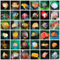
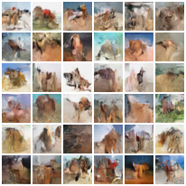
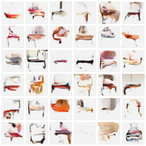
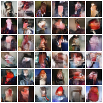
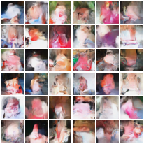
This fact means that we can easily generate datasets of varying difficulty by changing the temperature . For example, in Figure 2 we show samples generated by a flow model (see Section 4 for implementation details) trained on the Fashion-MNIST dataset at various values of temperature and the associated Bayes error. As , the distribution concentrate on the mode of the distributions , making the classification tasks easy, whereas when gets large, the distributions become more uniform, making classification more challenging. In practice, this can be used to generate datasets with almost arbitrary Bayes error: for any prescribed error in the range of the map , we can numerically invert this map to find for which .
4 Empirical investigation
4.1 Setup
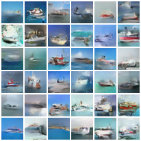
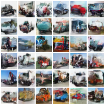
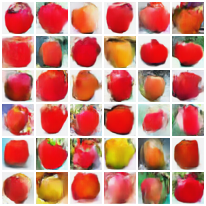
Datasets and data preparation. We train flow models on a wide variety of standard benchmark datasets: MNIST LeCun98, Extended MNIST (EMNIST) Cohen17, Fashion MNIST Xiao17, CIFAR-10 Krizhevsky09, CIFAR-100 Krizhevsky09, SVHN Netzer11, and Kuzushiji-MNIST clanuwat2018deep. The EMNIST dataset has several different splits, which include splits by digits, letters, merge, class, and balanced. The images in MNIST, Fashion-MNIST, EMNIST, and Kuzushiji-MNIST are padded to -by- pixels.222Glow implementation requires the input dimension to be power of .
We remark that we observe our Bayes error estimator runs efficiently when the input is of dimension -by--by-. However it is in general highly memory intensive to run the HDR integration routine on significantly larger datasets, e.g. when the input size grows to -by--by-. As a consequence, in our experiments we only work on datasets of dimension no larger than -by--by-.
Modeling and training. The normalizing flow model we use in our experiments is a pytorch implementation GlowPytorch of Glow kingma2018glow. In all our the experiments, affine coupling layers are used, the number of steps of the flow in each level , the number of levels , and number of channels in hidden layers .
During training, we minimize the Negative Log Likelihood Loss (NLL)
| (16) |
As suggested in kingma2018glow, we also add a classification loss to predict the class labels from the second-to-last layer of the encoder with a weight of . During the experiments we traversed configurations with , and report the numbers produced by the model with the smallest NLL loss on the test set. Note here even though we add the classification loss in the objective as a regularizer, the model is selected based on the smallest NLL loss in the test set instead of the classification loss or the total loss. The training and evaluation are done on a workstation with 2 NVIDIA V100 GPUs.
4.2 Evaluating SOTA models against generated datasets

In this section, we use our trained flow models to generate synthetic versions of standard benchmark datasets, for which the Bayes error is known exactly. In particular, we generate synthetic versions of the MNIST and Fashion-MNIST datasets at varying temperatures. As we saw in Section 3.2, varying the temperature allows us to generate datasets with different difficulty. Here, we train a Wide-ResNet-28-10 model (i.e. a ResNet with depth 28 and width multiple 10) ZagoruykoK16; WideResNetPytorch on these datasets, and compare the test error to the exact Bayes error for these problems. This Wide-ResNet model (together with appropriate data augmentation) attains nearly state-of-the-art accuracy on the original Fashion-MNIST dataset RandomErasing, and so we expect that our results here reflect roughly the best accuracy presently attainable on these synthetic datasets as well. To make the comparison fair, we use a training set size of 60,000 to mimic the size of the original MNIST series of datasets.
The Bayes errors as well as the test errors achieved by the Wide-ResNet or ConvNet models are shown in Figure 3. As one would expect, the errors of trained models increase with temperature. It can be observed that Wide-ResNet and ConvNet are able to achieve close-to-optimal performance when the dataset is relatively easy, e.g., for MNIST and for Fashion-MNIST. The gap becomes more significant when the dataset is harder, e.g. for MNIST and for Fashion-MNIST.
For the Synthetic Fashion-MNIST dataset at temperature , in addition to the Wide-ResNet (WRN-28) considered above, we also trained three other architectures: a simple linear classifier (Linear), a 1-hidden layer ReLU network (MLP) with 500 hidden units, and a standard AlexNet convolutional architecture krizhevsky2012imagenet. The resulting test errors, as well as the Bayes error, are shown in Figure 4. We see that while the development of modern architectures has led to substantial improvement in the test error, there is still a reasonably large gap between the performance of the SOTA Wide-ResNet and Bayes optimality. Nonetheless, it is valuable to know that, for this task, the state-of-the-art has substantial room to be improved.

4.3 Dataset Hardness Evaluation
A important application of our Bayes error estimator is to estimate the inherent hardness of a given dataset, regardless of model. We run our estimator on several popular image classification corpora and rank them based on our estimated Bayes error. The results are shown in Table 1. As a comparison we also put the SOTA numbers in the table.
Before proceeding, we make two remarks. First, all of the Bayes errors reported here were computed using temperature . This is for two main reasons: 1) setting reflects the flow model attaining the lowest testing NLL, and hence is in some sense the “best” approximation for the true distribution, 2) the ordering of the hardness of classes is unchanged by varying temperature, and so taking is a reasonable default. Second, the reliability of the Bayes errors reported here as a measure of inherent difficulty are dependent on the quality of the approximate distribution ; if this distribution is not an adequate estimate of the true distribution , then it is possible that the Bayes errors do not accurately reflect the true difficulty of the original dataset. Therefore, we also report the test NLL for each model as a metric to evaluate the quality of the approximant .
First, we observe that, by and large, the estimated Bayes errors align well with SOTA. In particular, if we constrain the NLL loss to be smaller than , then ranking by our estimated Bayes error aligns exactly with SOTA.
Second, the NLL loss in MNIST, Fashion MNIST, EMNIST and Kuzushiji-MNIST is relatively low, suggesting a good approximation by normalizing flow. However corpora such as CIFAR-10, CIFAR-100, and SVHN may suffer from a lack of training samples. In general large NLL loss may be due to either insufficient model capacity or lack of samples. In our experiments, we always observe the Glow model is able to attain essentially zero error on the training corpus, so it is highly possible the large NLL loss is caused by the lack of training samples.
Third, for datasets such as MNIST, EMNIST (digits, letters, balanced), SVHN, Fashion-MNIST, Kuzushiji-MNIST, CIFAR-10, and CIFAR-100 the SOTA numbers are roughly the same order of magnitude as the Bayes error. On the other hand, for EMNIST (bymerge and byclass) there is still substantial gap between the SOTA and estimated Bayes errors. This is consistent with the fact that there is little published literature about these two datasets; as a result models for them are not as well-developed.
| Corpus | #classes | #samples | NLL | Bayes Error | SOTA Error PaperWithCode |
|---|---|---|---|---|---|
| MNIST | 10 | 60,000 | 8.00e2 | 1.07e-4 | 1.6e-3 Byerly2001 |
| EMNIST (digits) | 10 | 280,000 | 8.61e2 | 1.21e-3 | 5.7e-3 Pad2020 |
| SVHN | 10 | 73,257 | 4.65e3 | 7.58e-3 | 9.9e-3 Byerly2001 |
| Kuzushiji-MNIST | 10 | 60,000 | 1.37e3 | 8.03e-3 | 6.6e-3 Gastaldi17 |
| CIFAR-10 | 10 | 50,000 | 7.43e3 | 2.46e-2 | 3e-3 foret2021sharpnessaware |
| Fashion-MNIST | 10 | 60,000 | 1.75e3 | 3.36e-2 | 3.09e-2 Tanveer2006 |
| EMNIST (letters) | 26 | 145,600 | 9.15e2 | 4.37e-2 | 4.12e-2 kabir2007 |
| CIFAR-100 | 100 | 50,000 | 7.48e3 | 4.59e-2 | 3.92e-2 foret2021sharpnessaware |
| EMNIST (balanced) | 47 | 131,600 | 9.45e2 | 9.47e-2 | 8.95e-2 kabir2007 |
| EMNIST (bymerge) | 47 | 814,255 | 8.53e2 | 1.00e-1 | 1.90e-1 Cohen17 |
| EMNIST (byclass) | 62 | 814,255 | 8.76e2 | 1.64e-1 | 2.40e-1 Cohen17 |
4.4 Hardness of Classes
In addition to measuring the difficulty of classification tasks relative to one another, it also may be of interest to evaluate the relative difficulty of individual classes within a particular task. A natural way to do this is by looking at the error of one-vs-all classification tasks. Specifically, for a given class , we consider drawn from the distribution , and from . The optimal Bayes classifier in this task is
Unfortunately, in this case, the Bayes error cannot be computed with HDR integration, since is now a mixture of Gaussians. However, we can get a reasonable approximation for the error (though less accurate than exact integration would be) in this case using a simple Monte Carlo estimator: , where as prescribed above.
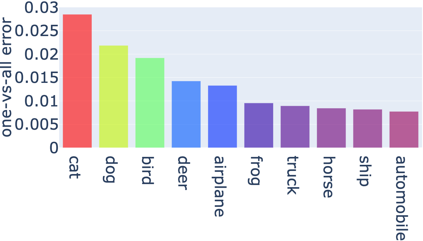
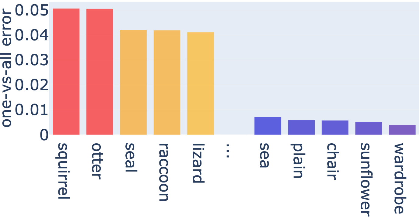
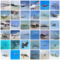
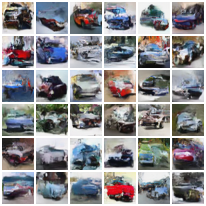
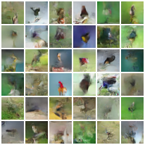
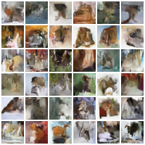
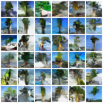
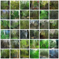
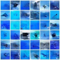
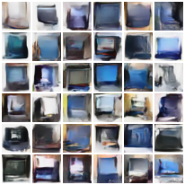
The one-vs-all errors by class on CIFAR are shown in Figure 5. It is observed that the errors between the hardest class and the easiest class is huge. On CIFAR-100 the error of the hardest class, squirrel, is almost times that of the easiest class, wardrobe.
5 Limitations, Societal Impact, and Conclusion
In this work, we have proposed a new approach to benchmarking state-of-the-art models. Rather than comparing trained models to each other, our approach leverages normalizing flows and a key invariance result to be able to generate benchmark datasets closely mimicking standard benchmark datasets, but with exactly controlled Bayes error. This allows us to evaluate the performance of trained models on an absolute, rather than relative, scale. In addition, our approach naturally gives us a method to assess the relative hardness of classification tasks, by comparing their estimated Bayes errors.
While our work has led to several interesting insights, there are also several limitations at present that may be a fruitful source of future research. For one, it is possible that the Glow models we employ here could be replaced with higher quality flow models, which would perhaps lead to better benchmarks and better estimates of the hardness of classification tasks. To this end, it is possible that the well-documented label noise in standard datasets contributes to our inability to learn higher-quality flow models NorthcuttAM2021. To the best of our knowledge, there has not been significant work using normalizing flows to accurately estimate class-conditional distributions for NLP datasets; this in itself would be an interesting direction for work. Second, a major limitation of our approach is that there isn’t an immediately obvious way to assess how well the Bayes error of the approximate distribution estimates the true Bayes error . Theoretical results which bound the distance between these two quantities, perhaps in terms of a divergence , would be of great interest here.
As detailed in VarshneyKS2019, there may be pernicious impacts of the common task framework and the so-called Holy Grail performativity that it induces. For example, a singular focus by the community on the leaderboard performance metrics without regard for any other performance criteria such as fairness or respect for human autonomy. The work here may or may not exacerbate this problem, since trying to approach fundamental Bayes limits is psychologically different than trying to do better than SOTA. As detailed in Varshney2020, the shift from competing against others to a pursuit for the fundamental limits of nature may encourage a wider and more diverse group of people to participate in ML research, e.g. those with personality type that has less orientation to competition. It is still to be investigated how to do this, but the ability to generate infinite data of a given target difficulty (yet style of existing datasets) may be used to improve the robustness of classifiers and perhaps decrease spurious correlations.
Checklist
-
1.
For all authors…
-
(a)
Do the main claims made in the abstract and introduction accurately reflect the paper’s contributions and scope? [Yes]
-
(b)
Did you describe the limitations of your work? [Yes] See Section 5
-
(c)
Did you discuss any potential negative societal impacts of your work? [Yes] See Section 5
-
(d)
Have you read the ethics review guidelines and ensured that your paper conforms to them? [Yes]
-
(a)
-
2.
If you are including theoretical results…
-
(a)
Did you state the full set of assumptions of all theoretical results? [Yes]
-
(b)
Did you include complete proofs of all theoretical results? [Yes] See the Appendix.
-
(a)
-
3.
If you ran experiments…
-
(a)
Did you include the code, data, and instructions needed to reproduce the main experimental results (either in the supplemental material or as a URL)? [No] We are about to open source our code repo.
-
(b)
Did you specify all the training details (e.g., data splits, hyperparameters, how they were chosen)? [Yes]
-
(c)
Did you report error bars (e.g., with respect to the random seed after running experiments multiple times)? [No] The Bayes Error Estimator is pretty accurate as shown in Figure 1. The normalizing flow is in general slow to train multiple times on all datasets and report an error bar w.r.t. random seeds.
-
(d)
Did you include the total amount of compute and the type of resources used (e.g., type of GPUs, internal cluster, or cloud provider)? [Yes] See Section 4
-
(a)
-
4.
If you are using existing assets (e.g., code, data, models) or curating/releasing new assets…
-
(a)
If your work uses existing assets, did you cite the creators? [Yes]
-
(b)
Did you mention the license of the assets? [No] The datasets and code repos we are using are well known and we provided the references so that readers can find the corresponding licenses.
-
(c)
Did you include any new assets either in the supplemental material or as a URL? [No] We are about to open source our code repo.
-
(d)
Did you discuss whether and how consent was obtained from people whose data you’re using/curating? [No] The data we are using are all well-known open-sourced sets with proper licenses. Readers can refer to our citation for the details.
-
(e)
Did you discuss whether the data you are using/curating contains personally identifiable information or offensive content? [No] To the best of our knowledge, the data we are using do not contain personally identifiable information or offensive content.
-
(a)
-
5.
If you used crowdsourcing or conducted research with human subjects…
-
(a)
Did you include the full text of instructions given to participants and screenshots, if applicable? [N/A]
-
(b)
Did you describe any potential participant risks, with links to Institutional Review Board (IRB) approvals, if applicable? [N/A]
-
(c)
Did you include the estimated hourly wage paid to participants and the total amount spent on participant compensation? [N/A]
-
(a)
Appendix A Proof of Proposition 1
Proof.
Throughout, we will use to denote the absolute value determinant of the Jacobian . Using the representation derived in [noshad2019learning], we can write the Bayes error as
| (17) |
Then if , we have that , and . Hence
By the Inverse Function Theorem, , and so we get
which completes the proof. ∎
Appendix B Further empirical results
In this supplementary material, we include further empirical results.