Evaluating the quantum Ziv–Zakai bound in noisy environments

Fundamental principles of quantum mechanics, e.g., Heisenberg uncertainty, impose ultimate precision limits on the parameter estimation 1 ; 2 ; 3 ; 4 . To efficiently quantify the minimum estimation error in quantum metrology, the quantum Cramér-Rao bound (QCRB) is particularly famous for giving a method to derive the asymptotically attainable estimation precision 1 ; 5 ; 6 ; 7 . More specifically, the QCRB is inversely proportional to the quantum Fisher information (QFI), so that such a lower bound plays more important role in metrologic applications, such as quantum sensing 8 ; 9 ; 10 , gravitational wave detection 11 ; 12 and optical imaging 13 ; 14 ; 15 . Especially, with the help of the multiparameter QCRB corresponding to the QFI matrix, T.J. Proctor et al. investigated the multiparameter estimation in the framework of networked quantum sensors 16 . However, the QCRB is asymptotically tight only under the limit of infinitely many trials, which may seriously underestimate the estimation precision if the likelihood function is highly non-Gaussian 17 ; 18 ; 19 ; 20 ; 21 . Thus, it is still an open problem to solve the bound of evaluation accuracy for the limited number of tests or non-Gaussian cases.

For this reason, the quantum Weiss-Weinstein bound 18 and the QZZB 17 ; 19 are often viewed as an alternative candidate to solve the problem mentioned above. Compared to the former, the later has been widely studied because it is relatively easy to calculate. For the single-parameter estimation, V. Giovannetti et al. demonstrated how to obtain a lower bound from prior information regimes, indicating that the sub-Heisenberg estimation strategies are ineffective 19 . After that, by relying on the QZZB, Y. Gao and H. Lee theoretically derived the generalized limits for parameter sensitivity when considering the implementations of adaptive measurements, and they found that the precision of phase estimation with several known states cannot be superior to the Heisenberg limit 21 . By extending the QZZB into the multiparameter cases, Y. R. Zhang and H. Fan presented two kinds of metrological lower bounds using two different approximations proposed by Tsang even in noisy systems 20 . They showed the advantage of simultaneous estimation over optimal individual one, but the achievable bounds may be not tight either due to some approximation methods used. Additionally, in order to further develop the QZZB, D. W. Berry et al. proposed a novel lower bound for phase waveform estimation as an application of multiparameter case via the quantum Bell-Ziv–Zakai bound 22 . These results show that the QZZB become one of the promising candidates to attain the lower bound of the (multi-)parameter estimation for tightness.

On the other hand, for realistic scenarioes, because of the inevitable interactions between the quantum system and its surrounding noisy environment, the corresponding estimation precision would be reduced, which has been studied extensively in recent years 23 ; 24 ; 25 ; 26 ; 27 ; 28 ; 29 ; 30 ; 31 . In particular, since a variational method was first proposed by Escher 24 , the analytical QCRB of single-(or multiple-) parameter estimation in noisy environment can be derived effectively 32 ; 33 ; 34 . We also noticed that the effects of noisy environment on the single-estimation performance of the QZZB has not been studied before. Thus, in this paper, we shall focus on the general derivation of the QZZB in the presence of both the photon loss and the phase diffusion with the help of the technique of integration within an ordered product of operators (IWOP) 35 ; 36 ; 37 ; 38 ; 39 ; 40 ; 41 . Further, we also present the estimation performance of the QZZB in the presence of the two noise scenarioes when given some optical resources, such as the CS, the SMSVS and the TMSVS. The results show that for the the photon-loss scenario, the CS shows the better estimation performance of the QZZB, due to its robustness against the photon losses, when comparing to the cases of both the SMSVS and the TMSVS. While for the phase-diffusion scenario, the estimation performance of the QZZB for the CS can be outperformed by that for the TMSVS at the large range of the phase-diffusion strength.

This paper is arranged as follows. In section II, we briefly review the known results of the QZZB. Based on the variational method and the IWOP technique, in section III and IV, we respectively derive the tight QZZB in the presence of the photon-loss and phase-diffusion scenarioes, and then also investigate the estimation performance of the QZZB with the two noise scenarioes for given some Gaussian states, such as the CS, the SMSVS and the TMSVS. Finally, the main conclusions are drawn in the last section.

It is pointed out that the QZZB can show much tighter than the conventional QCRB for the highly non-Gaussian regime 17 ; 18 ; 19 . So, in this section, we briefly review the known results of the quantum parameter estimation based on the QZZB. From the perspective of a classical parameter-estimated theory, let $x$ be the unknown parameter to be estimated, $y$ be the observation with finite measurements, and $X\left(y\right)$ be an estimator of $x$ constructed from the observation $y$. Thus, the parameter sensitivity of $x$ can be quantified using the weighted root mean square error

where $p\left(y|x\right)$ represents the condition probability density of achieving the observation $y$ given $x$, and $p(x)$ represents the prior probability density. According to Refs. 42 ; 43 ; 44 ; 45 , a classical Ziv-Zakai bound, i.e., a lower bound for $\sum$, can be given by

where $\Pr\nolimits_{e}^{el}(x,x+\beta)$ represents the minimum error probability for the binary decision problem with an equally prior probability, and $\chi$ is the so-called optional valley-filling operation, i.e., $\chi f(\beta)\equiv\max_{\eta\geq 0}f(\beta+\eta)$, which renders the bound tighter but harder to calculate 17 ; 42 ; 43 .

Likewise, for the quantum parameter-estimated theory, let $\hat{\rho}\left(x\right)$ be the density operator as a function of the unknown parameter $x$, and let $\hat{E}(y)$ be the positive operator-valued measure so as to establish the measurement model. Then, the observation density is denoted as

with a symbol of Tr being the operator trace. Thus, according to Refs. 17 ; 20 ; 46 , a lower bound of the minimum error probability $\Pr\nolimits_{e}^{el}(x,x+\beta)$ is given by

with the trace norm $\left\|\hat{O}\right\|_{1}=$Tr$\sqrt{\hat{O}^{\dagger}\hat{O}}$ and the Uhlmann fidelity $F(\hat{\rho}\left(x\right),\hat{\rho}\left(x+\beta\right))=(Tr\sqrt{\sqrt{\hat{\rho}\left(x\right)}\hat{\rho}\left(x+\beta\right)\sqrt{\hat{\rho}\left(x\right)}})^{2}$.

Now, let us assume that an unknown parameter $x$ is encoded into the quantum state $\hat{\rho}\left(x\right)$, which can be presented in terms of an unitary evolution

where $\hat{\rho}$ is the initial state and $\hat{H}$ is the effective Hamiltonian operator. Thus, it can be seen that $F(\hat{\rho}\left(x\right),\hat{\rho}\left(x+\beta\right))\geq\left|\text{Tr}(\hat{\rho}e^{-i\hat{H}\beta})\right|^{2}$ 47 . After assuming that the prior probability density $p(x)$ is the uniform window with the mean $\mu$ and the width $W$ denoted as

and omitting the optional $\chi$, one can obtain the QZZB, i.e. 17 ,

where $F(\beta)\equiv\left|\text{Tr}(\hat{\rho}e^{-i\hat{H}\beta})\right|^{2}$ is a lower bound of the fidelity $F(\hat{\rho}\left(x\right),\hat{\rho}\left(x+\beta\right)).$ For the initial pure state $\hat{\rho},$ $F(\beta)$ is the fidelity between $\hat{\rho}\left(x\right)$ and $\hat{\rho}\left(x+\beta\right).$ In the following, we would take the effects of the environment on the QZZB into account, since the encoding process of the quantum state $\hat{\rho}$ to unknown parameter $x$ is inevitably affected by the environment, such as the photon losses and the phase diffusion.

In the case of photon losses, the encoding process of the quantum state to unknown parameter $x$ no longer satisfies unitary evolution, so that the QZZB can not be directly derived by using Eq. (7). Fortunately, similar to obtain the upper bound for QFI proposed by Escher with the assistance of an variational method 24 ; 48 , combining with the IWOP technique, here we shall present the derivation of the QZZB in the presence of photon losses.

In order to change the encoding process into the unitary evolution $\hat{U}_{S+E}\left(x\right)$, the basic idea is to introduce additional degrees of freedom, acting as an environment $E$ for the system $S$. When given an initial pure state $\hat{\rho}_{S}=\left|\psi_{S}\right\rangle\left\langle\psi_{S}\right|$ of a probe system $S,$ the encoding process of the initial pure state $\hat{\rho}_{S}$ is the non-unitary evolution under the photon losses. So, it is necessary to expand the size of the Hilbert space $S$ together with the photon losses environment space $E$. After the quantum state in the enlarged space $S+E$ goes through the unitary evolution $\hat{U}_{S+E}\left(x\right),$ one can obtain

where $\hat{\rho}_{E_{0}}=\left|0_{E}\right\rangle\left\langle 0_{E}\right|$ is the initial state of the photon losses environment space $E$, $\hat{\rho}_{E_{l}}=\left|l_{E}\right\rangle\left\langle l_{E}\right|$ is the orthogonal basis of the $\hat{\rho}_{E_{0}},$ and $\hat{\Pi}_{l}\left(x\right)$ is the Kraus operator acting on the $\hat{\rho}_{S},$ which can be described as

with the strength of photon losses $\eta$, the variational parameter $\lambda_{1},$ and the photon number operator $\hat{n}=\hat{a}^{{\dagger}}\hat{a}$. Note that $\eta=0$ and $\eta=1$ respectively correspond to complete absorption and non-loss case. According to the Uhlmann’s theorem 49 , thus, the fidelity for the enlarged system $S+E$ with photon losses can be given by

where

corresponds to the lower bound of the fidelity in photon losses with $\hat{Z}$ defined as

By invoking the IWOP technique and Eqs. (9) and (12), one can respectively obtain the operator identities, i.e.,

where $:\cdot:$ denotes the symbol of the normal ordering form. The more details for the derivation can be seen in the Appendix A. Thus, based on Eqs. (13) and (14), the lower bound of the fidelity, i.e., $F_{Q_{1}}(\hat{\rho}_{S+E}\left(x\right),\hat{\rho}_{S+E}\left(x+\beta\right))\equiv F_{Q_{1}}\left(\beta\right),$ can be given by

From Eq. (15), it should be noted that, when the variational parameter $\lambda_{1}$ takes the optimal value $\lambda_{1opt}$, $F_{Q_{1}}\left(\beta\right)$ can reach the maximum value, which is the fidelity (denoted as $F_{L_{1}}(\beta)$) in the photon-loss environment. In this situation, the lower limit of the minimum error probability $\Pr\nolimits_{e_{L_{1}}}^{el}(x,x+\beta)$ under the photon losses can be expressed as

According to Eq. (6), finally, we can obtain the QZZB in the presence of the photon-loss environment

Futhermore, by utilizing the inequalities 17

with the fidelity $F_{L_{1}}(\beta)$ satisfying the conditions of $0\leq F_{L_{1}}(\beta)\leq 1$ and $0\leq\beta\leq W,$ the Eq. (17) can be further rewritten as

where $\tilde{F}_{1}(\beta)=\frac{W}{16}F_{L_{1}}(\beta)\sin(\pi\beta/W)$ is denoted as the generalized fidelity under the photon-loss case.

In this situation, here we shall consider the QZZB under the photon losses when inputting three initial states of the probe system $S$, involving the CS (denoted as $\left|\psi_{S}\left(\alpha\right)\right\rangle$), the SMSVS (denoted as $\left|\psi_{S}\left(r_{1}\right)\right\rangle$) and the TMSVS (denoted as $\left|\psi_{S}\left(r_{2}\right)\right\rangle$). Following the approach proposed by Tsang 17 , and according to Eq. (19), one can respectively derive the QZZB of the given initial states in the presence of the photon-loss environment, i.e. [see Appendix B],

where $N_{\alpha}=\left|\alpha\right|^{2}$ is the mean photon number of the CS, erfi$(\epsilon)\equiv(2/\sqrt{\pi})\int_{0}^{\epsilon}\exp(t^{2})dt,$ and the generalized fidelities of both the SMSVS and the TMSVS are respectively given by

with

Note that $F_{Q_{1}}\left(\beta\right)_{(r_{1})}$=$\left.1\right/\left|\sqrt{1+N_{r_{1}}\left[1-\Upsilon^{2}(\eta,\beta,\lambda_{1})\right]}\right|^{2}$ with the mean photon number $N_{r_{1}}$=$\sinh^{2}r_{1}$, and $F_{Q_{1}}\left(\beta\right)_{(r_{2})}$=$\left.1\right/\left|1+\left.N_{r_{2}}\left[1-\Upsilon(\eta,\beta,\lambda_{1})\right]\right/2\right|^{2}$ with the mean photon number $N_{r_{2}}$=$2\sinh^{2}r_{2}$ are respectively the lower bound of the fidelity for the SMSVS and the TMSVS, as well as $\Upsilon(\eta,\beta,\lambda_{1})$=$\eta e^{-i\beta}+\left(1-\eta\right)e^{i\beta\lambda_{1}}$. In particular, according to Eq. (20), when $\eta=1$ corresponding to the non-loss case, the corresponding QZZB for the input CS is consistent with the previous work 17 .

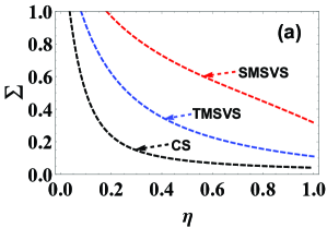
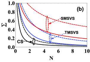
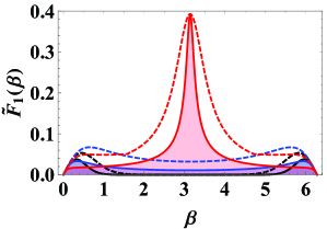
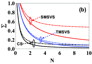
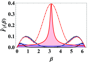
In order to visually see the effects of photon losses on the QZZB, at a fixed value of $N=5,$ we plot the QZZB $\sum$ as a function of the photon-loss strength $\eta$ for several different states, involving the CS (black dashed line), the SMSVS (red dashed line), and the TMSVS (blue dashed line), as shown in Fig. 1(a). The results show that, with the decrease of $\eta,$ the value of the QZZB for the given states increases. Especially, compared to the another states, the QZZB for the CS increases relatively slowly, which means that the CS as the input is more conducive to reducing the estimation uncertainty under the photon losses. Further, to evaluate the gap between the ideal and photon-loss cases, at a fixed $\eta=0.5,$ we also show the QZZB $\sum$ as a function of the mean photon number $N$ for several input resources, i.e., the CS (black lines), the SMSVS (red lines), and the TMSVS (blue lines), as pictured in Fig. 1(b). For comparison, the solid lines correspond to the ideal cases. It is clearly seen that, for the CS, the gap between ideal and photon-loss cases is the smallest, which implies that the CS is more robust against photon losses than other input resources at the same conditions. Moreover, compared with both the CS and the TMSVS, the estimation performance of the QZZB for the SMSVS is the worst under the ideal or photon-loss cases. The reasons for these phenomenons can be explained in terms of the generalized fidelity $\tilde{F}_{1}(\beta)$ given in Eq. (19). For this purpose, at fixed values of $N=5$ and $\eta=0.5,$ we consider the generalized fidelity $\tilde{F}_{1}(\beta)$ as a function of $\beta$ for several different initial states, including the CS (black lines), the SMSVS (red lines), and the TMSVS (blue lines), as shown in Fig. 2. According to Eq. (19), the area enclosed by the curve lines and abscissa is the value of the QZZB, which implies that the larger the area, the worse the estimation performance. Taking the ideal case as a concrete example, we can clearly see that the area for the SMSVS (red region) is the largest, followed by that for the TMSVS (blue region), and then that for the CS (black region), which is also true for the photon losses.

More recently, the effects of phase diffusion on the QCRB have been studied in Ref. 48 , and they found that compared with photon losses, the existence of phase diffusion has a greater influence on the QCRB. Naturally, the question arises: what are the effects of phase diffusion on the performance of the QZZB? To answer such a question, in this section, we first derive the general form of the QZZB in the presence of phase diffusion by using the variational method and the IWOP technique, and then show the performance of the QZZB with the given states including the $\left|\psi_{S}\left(\alpha\right)\right\rangle$, the $\left|\psi_{S}\left(r_{1}\right)\right\rangle$ and the $\left|\psi_{S}\left(r_{2}\right)\right\rangle$.

Generally speaking, the phase diffusion process can be modeled using the interaction between the probe system $S$ and the environment $E^{\prime}$, which can be described as

where $\kappa$ denotes the strength of phase diffusion and $\hat{q}_{E^{\prime}}=(\hat{a}_{E^{\prime}}+\hat{a}_{E^{\prime}}^{\dagger})/\sqrt{2}$ is the dimensionless position operator of the mirror. On this background, the density operator $\hat{\rho}_{S+E^{\prime}}^{\prime}\left(x\right)$ in the whole system $S+E^{\prime}$ can be given by

where $\hat{\rho}_{S}$ is the same as the aforementioned definition given in Eq. (8), $\hat{U}_{S+E^{\prime}}^{\prime}\left(x\right)=\exp\left(-ix\hat{n}\right)\exp(i2\kappa\hat{n}\hat{q}_{E^{\prime}})$ is the corresponding unitary operator of the combined system $S+E^{\prime},$ and $\hat{\rho}_{E_{0}^{\prime}}=\left|0_{E^{\prime}}\right\rangle\left\langle 0_{E^{\prime}}\right|$ is the initial state of the phase-diffusion environment, which is often assumed to be the ground state of a quantum oscillator. It is clearly seen from Eq. (24) that the density operator $\hat{\rho}_{S+E^{\prime}}^{\prime}\left(x\right)$ can be viewed as the purifications of the probe state $\hat{\rho}_{S}\left(x\right)$, which is given by 48

where $\rho_{m,n}=\left\langle m\right|\hat{\rho}_{S}\left|n\right\rangle$ is the matrix element of the initial state for the probe system $S$. Thus, according to Eq. (24), under the asymptotic condition of $\sqrt{2}\kappa n\gg 1$, the purified unitary evolution can integrally be written as 48

where $\hat{u}_{E^{\prime}}(x)=e^{\left.ix\lambda_{2}\hat{p}_{E^{\prime}}\right/2\kappa}$ is the unitary operator with $\lambda_{2}$ being a variational parameter and $\hat{p}_{E^{\prime}}=(\hat{a}_{E^{\prime}}-\hat{a}_{E^{\prime}}^{\dagger})/i\sqrt{2}$ being the dimensionless momentum operator of the mirror, which acts only on the phase-diffusion environment $E^{\prime},$ and connects two purifications $\hat{\rho}_{S+E^{\prime}}^{\prime}\left(x\right)$ and $\hat{\rho}_{S+E^{\prime}}^{\prime\prime}\left(x\right)$ of the same probe state $\hat{\rho}_{S}\left(x\right)$.

Based on the Uhlmann’s theorem 49 , the fidelity in the phase-diffusion environment $E^{\prime}$ can be given by

where $F_{Q_{2}}(\hat{\rho}_{S+E^{\prime}}^{\prime\prime}\left(x\right),\hat{\rho}_{S+E^{\prime}}^{\prime\prime}\left(x+\beta\right))\equiv F_{Q_{2}}\left(\beta\right)$ is the lower bound of the fidelity in the phase-diffusion environment $E^{\prime},$ which can be derived as

with $\Theta(\kappa,\beta,\lambda_{2})=e^{\left.-\beta^{2}\lambda_{2}^{2}\right/8\kappa^{2}}$. One can refer to the Appendix C for more details of the corresponding derivation in Eq. (28).

Likewise, if the variational parameter $\lambda_{2}$ takes the optimal value $\lambda_{2opt}$, then $F_{Q_{2}}\left(\beta\right)$ can achieve the maximum value, which is the fidelity in the phase-diffusion environment $F_{L_{2}}(\beta).$ Further, the lower limit of the minimum error probability $\Pr\nolimits_{e_{L_{2}}}^{el}(x,x+\beta)$ in the presence of the phase-diffusion environment $E^{\prime}$ can be given by

Similar to how we get the Eq. (19), the QZZB in the presence of the phase-diffusion environment can be denoted as

By using the Eq. (18), finally, the Eq. (30) can be rewritten as

where $\tilde{F}_{2}(\beta)=\frac{W}{16}F_{L_{2}}(\beta)\sin(\pi\beta/W)$ is also denoted as the generalized fidelity under the phase-diffusion case.

Next, let us consider the performance of the QZZB with the given states including the $\left|\psi_{S}\left(\alpha\right)\right\rangle$, the $\left|\psi_{S}\left(r_{1}\right)\right\rangle$ and the $\left|\psi_{S}\left(r_{2}\right)\right\rangle$. According to the Eq. (31), one can respectively derive the QZZB of these given states in the presence of the phase-diffusion environment, i.e.,

where we have set

with

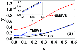
For the sake of clearly seeing the effects of phase diffusion on the QZZB, at a fixed value of $N=5,$ we plot the QZZB $\sum$ as a function of the phase-diffusion strength $\kappa$ for the given states including the CS (black dot-dashed line), the SMSVS (red dot-dashed line) and the TMSVS (blue dot-dashed line), as shown in Fig. 3(a). It is clear that the value of the QZZB for the given states increases with the increase of $\kappa$. In particular, compared to other states, the corresponding QZZB for the SMSVS is relatively larger and increases rapidly as the phase-diffusion strength $\kappa$ increases, which means that both the CS and the TMSVS instead of the SMSVS is a better choice to the robustness against the phase diffusion. More precisely, at the rang of $0\leqslant\kappa\leqslant 0.41,$ the value of the QZZB for the CS can be lower than that for the TMSVS, but the former can be larger than the latter when $\kappa$ is greater than $0.41$. This phenomenon means that the CS can be more sensitive to the phase-diffusion environment compared to the TMSVS [see Fig. 3(b)]. In addition, under the phase diffusion processes (e.g., $\kappa=0.2$), we further consider the QZZB $\sum$ as a function of the mean photon number $N$ for the CS (black lines), the SMSVS (red lines), and the TMSVS (blue lines), as shown in Fig. 3(b). As a comparison, the ideal cases (solid lines) are also plotted here. It is shown that, the gap with the SMSVS (red lines) between the ideal and phase diffusion cases is the largest, which means that the SMSVS is more sensitive to the phase diffusion than other states. We also find that the gap with the TMSVS is smaller than the one with the CS when given the same mean photon number $N$, which does exist in the case of photon losses. Even so, the estimation performance of the QZZB for the CS is superior to that for the TMSVS under the phase diffusion. Similar to Fig. 2, in order to better explain these phenomena, at fixed values of $N=5$ and $\kappa=0.2,$ Fig. 4 shows the generalized fidelity $\tilde{F}_{2}(\beta)$ as a function of $\beta$, in which the area enclosed by the curve lines and abscissa is the value of the QZZB. Likewise, by taking the phase diffusion as an example, the area for the SMSVS (red region) is the largest, followed by that for the TMSVS (blue region), and then that for the CS (black region), which implies that the CS shows the best estimation performance in the presence of the phase diffusion.

In summary, we have presented the estimation performance of the QZZB in noisy systems with several different Gaussian resources, including the CS, the SMSV and the TMSV. One of the major contributions showed in this paper is that the analytical expression of the QZZB is completely derived in the presence of the photon losses. It is shown that the estimation performance of the QZZB is related to the generalized fidelity, which can be used to explain the phenomenon that the QZZB for both the CS and the TMSVS performs better than that for the SMSVS, especially for the best performance with inputting the CS. Furthermore, we also investigate the effects of the phase diffusion systems on the QZZB with the same Gaussian resources. It is found that the CS as the initial state can show the better estimation performance of the QZZB at the small range of the phase-diffusion strength ($0\leqslant\kappa\leqslant 0.41$), but for the large range of the phase-diffusion strength $\left(\kappa>0.41\right),$ its estimation performance can be exceeded by that for the TMSVS. Finally, we should mention that it is impossible for investigating the optimal estimation performance by using the QZZB 20 , which is still a crucial problem for the future work.

Appendix A: The Proof of Eqs. (13) and (14)

By using the completeness relation of Fock states, one can obtain

where we have utilized the IWOP technique and the normal ordering form of the vacuum projection operator 36

Then, using Eq. (A1), one can further derive the operator $\hat{Z}$, i.e.,

where we have utilized the following operator identity about $e^{\lambda\hat{a}^{\dagger}\hat{a}}$ , i.e.,

to remove the symbol of normal ordering.

Appendix B: The QZZB for the CS in the presence of the photon losses environment

Based on Eq. (15), one can get the lower bound of the fidelity for the CS $\left|\psi_{S}\left(\alpha\right)\right\rangle$ under the photon-loss environment

The value of the variational parameter $\lambda_{1}$ that maximizes the lower bound is $\lambda_{1opt}=0,$ which yields the fidelity for the CS $\left|\psi_{S}\left(\alpha\right)\right\rangle$, i.e.,

Thus, substituting Eq. (B2) into Eq. (19), and $W=2\pi$, one can get

Changing the integral variable $\beta$ to $s\equiv\cos(\beta/2)$ and utilizing the identity $\cos\beta=2\cos^{2}(\beta/2)-1,$ one can finally obtain the QZZB for the CS in the presence of the photon-loss environment

Next, using the completeness relation of coherent states, the SMSVS $\left|\psi_{S}\left(r_{1}\right)\right\rangle$ can be expanded in the basis of the CS,

References

- (1) X. M. Lu, and X. G. Wang, “Incorporating Heisenberg’s Uncertainty Principle into Quantum Multiparameter Estimation,” Phys. Rev. Lett. 126, 120503 (2021).
- (2) M. Tsang, F. Albarelli, and A. Datta, “Quantum Semiparametric Estimation,” Phys. Rev. X 10, 031023 (2020).
- (3) A. Rath, C. Branciard, A. Minguzzi, and B. Vermersch, “Quantum Fisher Information from Randomized Measurements,” Phys. Rev. Lett. 127, 260501 (2021).
- (4) X. Yu, X. Zhao, L. Y. Shen, Y. Y. Shao, J. Liu, and X. G. Wang, “Maximal quantum Fisher information for phase estimation without initial parity,” Opt. Express 26, 16292 (2018).
- (5) S. L. Braunstein and C. M. Caves, “Statistical Distance and the Geometry of Quantum States,” Phys. Rev. Lett. 72, 3439 (1994).
- (6) Y. Yang, S. H. Ru, M. An, Y. L. Wang, F. R. Wang, P. Zhang, and F. L. Li, “Multiparameter simultaneous optimal estimation with an SU(2) coding unitary evolution,” Phys. Rev. A 105, 022406 (2022).
- (7) L. L. Guo, Y. F. Yu, and Z. M. Zhang, “Improving the phase sensitivity of an SU(1,1) interferometer with photon-added squeezed vacuum light,” Opt. Express 26, 29099 (2018).
- (8) C. Oh, C. Lee, S. H. Lie, and H. Jeong, “Optimal Distributed Quantum Sensing Using Gaussian States,” Phys. Rev. Research 2, 023030 (2020).
- (9) Y. Xia, W. Li, Q. T. Zhuang, and Z. S. Zhang, “Quantum-Enhanced Data Classification with a Variational Entangled Sensor Network,” Phys. Rev. X 11, 021047 (2021).
- (10) X. Guo, C. R. Breum, J. Borregaard, S. Izumi, M. V. Larsen, T. Gehring, M. Christandl, J. S. Neergaard-Nielsen, and U. L. Andersen, “Distributed Quantum Sensing in a Continuous-Variable Entangled Network,” Nat. Phys. 16, 281 (2020).
- (11) R. Demkowicz-Dobrzański, K. Banaszek, and R. Schnabel, “Fundamental quantum interferometry bound for the squeezed-light-enhanced gravitational wave detector GEO 600,” Phys. Rev. A 88, 041802(R) (2013).
- (12) E. Oelker, L. Barsotti, S. Dwyer, D. Sigg, and N. Mavalvala, “Squeezed light for advanced gravitational wave detectors and beyond,” Opt. Express 22, 21106 (2014).
- (13) M. Tsang, R. Nair, and X. M. Lu, “Quantum Theory of Superresolution for Two Incoherent Optical Point Sources,” Phys. Rev. X 6, 031033 (2016).
- (14) R. Nair and M. Tsang, “Interferometric superlocalization of two incoherent optical point sources,” Opt. Express 24, 3684 (2016).
- (15) C. H. Oh, S. S. Zhou, Y. Wong, and L. Jiang, “Quantum Limits of Superresolution in a Noisy Environment,” Phys. Rev. Lett. 126, 120502 (2021).
- (16) T. J. Proctor, P. A. Knott, and J. A. Dunningham, “Multiparameter Estimation in Networked Quantum Sensors,” Phys. Rev. Lett. 120, 080501 (2018).
- (17) M. Tsang, “Ziv-Zakai Error Bounds for Quantum Parameter Estimation,” Phys. Rev. Lett. 108, 230401 (2012).
- (18) X. M. Lu, and M. Tsang, “Quantum Weiss-Weinstein bounds for quantum metrology,” Quantum Sci. Technol. 1, 015002 (2016).
- (19) V. Giovannetti, and L. Maccone, “Sub-Heisenberg Estimation Strategies Are Ineffective,” Phys. Rev. Lett. 108, 210404 (2012).
- (20) Y. R. Zhang, and H. Fan, “Quantum metrological bounds for vector parameters,” Phys. Rev. A 90, 043818 (2014).
- (21) Y. Gao, and H. Lee, “Generalized limits for parameter sensitivity via quantum Ziv–Zakai bound,” J. Phys. A: Math. Theor. 45, 415306 (2012).
- (22) D. W. Berry, M. Tsang, M. J. W. Hall, and H. M. Wiseman, “Quantum Bell-Ziv-Zakai Bounds and Heisenberg Limits for Waveform Estimation,” Phys. Rev. X 5, 031018 (2015).
- (23) A. Monras, and M. G. A. Paris, “Optimal Quantum Estimation of Loss in Bosonic Channels,” Phys. Rev. Lett. 98, 160401 (2007).
- (24) B. M. Escher, R. L. de Matos Filho, and L. Davidovich, “General framework for estimating the ultimate precision limit in noisy quantum-enhanced metrology,” Nat. Phys. 7, 406 (2011).
- (25) S. S. Zhou, M. Z. Zhang, J. Preskill, and L. Jiang, “Achieving the Heisenberg limit in quantum metrology using quantum error correction,” Nat. Commun. 9, 78 (2018).
- (26) Y. Gao, and R. M. Wang, “Variational limits for phase precision in linear quantum optical metrology,” Phys. Rev. A 93, 013809 (2016).
- (27) W. Ye, H. Zhong, Q Liao, D. Huang, L. Y. Hu, and Y. Guo, “Improvement of self-referenced continuous-variable quantum key distribution with quantum photon catalysis,” Opt. Express 27, 17186 (2019).
- (28) C. L. Latune, B. M. Escher, R. L. de Matos Filho, and L. Davidovich, “Quantum limit for the measurement of a classical force coupled to a noisy quantum-mechanical oscillator,” Phys. Rev. A 88, 042112 (2013).
- (29) M. G. Genoni, S. Olivares, and M. G. A. Paris, “Optical Phase Estimation in the Presence of Phase Diffusion,” Phys. Rev. Lett. 106, 153603 (2011).
- (30) M. Zwierz, and H. M. Wiseman, “Precision bounds for noisy nonlinear quantum metrology,” Phys. Rev. A 89, 022107 (2014).
- (31) H. Zhang, W. Ye, C. P. Wei, Y. Xia, S. K. Chang, Z. Y. Liao, and L. Y. Hu, “Improved phase sensitivity in a quantum optical interferometer based on multiphoton catalytic two-mode squeezed vacuum states,” Phys. Rev. A 103, 013705 (2021).
- (32) J. D. Yue, Y. R. Zhang, and H. Fan, “Quantum-enhanced metrology for multiple phase estimation with noise.” Sci. Rep. 4, 5933 (2014).
- (33) S. K. Chang, W. Ye, H. Zhang, L. Y. Hu, J. H. Huang, and S. Q. Liu, “Improvement of phase sensitivity in an SU(1,1) interferometer via a phase shift induced by a Kerr medium,” Phys. Rev. A 105, 033704 (2022).
- (34) H. Zhang, W. Ye, C. P. Wei, C. J. Liu, Z. Y. Liao, and L. Y. Hu, “Improving phase estimation using number-conserving operations,” Phys. Rev. A 103, 052602 (2021).
- (35) H. Y. Fan and H. R. Zaidi, “Application of IWOP technique to the generalized Weyl correspondence,” Phys. Lett. A 124, 303 (1987).
- (36) H. Y. Fan, H. L. Lu, and Y. Fan, “Newton-Leibniz integration for ket-bra operators in quantum mechanics and derivation of entangled state representations,” Ann. Phys. 321, 480 (2006).
- (37) W. Ye, H. Zhong, X. D. Wu, L. Y. Hu and Y. Guo, “Continuous-variable measurement-device-independent quantum key distribution via quantum catalysis,” Quantum Inf. Process. 19, 346 (2020).
- (38) H. Y. Fan, J. R. Klauder, “Eigenvectors of two particles’ relative position and total momentum,” Phys. Rev. A 49, 704 (1994).
- (39) M. M. Luo, Y. T. Chen, J. Liu, S. H. Ru, S. Y. Gao, “Enhancement of phase sensitivity by the additional resource in a Mach-Zehnder interferometer,” Phys. Lett. A 424, 127823 (2022).
- (40) Y. R. Zhang, L. H. Shao, Y. M. Li, and H. Fan, “Quantifying coherence in infinite-dimensional systems,” Phys. Rev. A 93, 012334 (2016).
- (41) S. K. Chang, C. P. Wei, H. Zhang, Y. Xia, W. Ye, and L. Y. Hu, “Enhanced phase sensitivity with a nonconventional interferometer and nonlinear phase shifter,” Phys. Lett. A 384, 126755 (2020).
- (42) J. Ziv and M. Zakai, “Some lower bounds on signal parameter estimation,” IEEE Trans. Inform. Theor. 15, 386 (1969).
- (43) L. P. Seidman, “Performance limitations and error calculations for parameter estimation,” Proc. IEEE 58, 644 (1970).
- (44) S. Bellini and G. Tartara, “Bounds on Error in Signal Parameter Estimation,” IEEE Trans. Commun. 22, 340 (1974);
- (45) E. Weinstein, “Relations between Belini-Tartara, Chazan-Zakai-Ziv, and Wax-Ziv lower bounds,” IEEE Trans. Inform. Theor. 34, 342 (1988).
- (46) C. A. Fuchs and J. van de Graaf, “Cryptographic distinguishability measures for quantum-mechanical states,” IEEE Trans. Inform. Theor. 45, 1216 (1999).
- (47) V. Giovannetti, S. Lloyd, and L. Maccone, “Quantum limits to dynamical evolution,” Phys. Rev. A 67, 052109 (2003).
- (48) B. M. Escher, L. Davidovich, N. Zagury, and R. L. de Matos Filho, “Quantum Metrological Limits via a Variational Approach,” Phys. Rev. Lett. 109, 190404 (2012).
- (49) A. Uhlmann, “The ‘transition probability’ in the state space of a *-algebra,” Rep. Math. Phys. 9, 273–279 (1976).