¹¹institutetext: INRIA, France Firstname.Name@inria.fr ²²institutetext: École Normale Supérieure Firstname.Name@ens.fr.

Evaluation of Chebyshev polynomials on intervals and application to root finding

Viviane Ledoux 1122 Guillaume Moroz 11

Abstract

In approximation theory, it is standard to approximate functions by polynomials expressed in the Chebyshev basis. Evaluating a polynomial $f$ of degree n given in the Chebyshev basis can be done in $O(n)$ arithmetic operations using the Clenshaw algorithm. Unfortunately, the evaluation of $f$ on an interval $I$ using the Clenshaw algorithm with interval arithmetic returns an interval of width exponential in $n$ . We describe a variant of the Clenshaw algorithm based on ball arithmetic that returns an interval of width quadratic in $n$ for an interval of small enough width. As an application, our variant of the Clenshaw algorithm can be used to design an efficient root finding algorithm.

Keywords:

Clenshaw algorithm Chebyshev polynomials Root finding Ball arithmetic Interval arithmetic.

1 Introduction

Clenshaw showed in 1955 that any polynomial given in the form

p(x)=\sum_{i=0}^{n}a_{i}T_{i}(x)

(1)

can be evaluated on a value $x$ with a single loop using the following functions defined by recurrence:

u_{k}(x)=\begin{cases}0&\text{if }k=n+1\\ a_{n}&\text{if }k=n\\ 2xu_{k+1}(x)-u_{k+2}(x)+a_{k}&\text{if }1\leq k<n\\ xu_{1}(x)-u_{2}(x)+a_{0}&\text{if }k=0\end{cases}

(2)

such that $p(x)=u_{0}(x)$ .

Unfortunately, if we use Equation (2) with interval arithmetic directly, the result can be an interval of size exponentially larger than the input, as illustrated in Example 1.

Example 1

Let $\varepsilon>0$ be a positive real number, and let $x$ be the interval $[\frac{1}{2}-\varepsilon,\frac{1}{2}+\varepsilon]$ of width $2\varepsilon$ . Assuming that $a_{n}=1$ , we can see that $u_{n-1}$ is an interval of width $4\varepsilon$ . Then by recurrence, we observe that $u_{n-k}$ is an interval of width at least $4\varepsilon F_{k}$ where ${(F_{n})}_{n\in\mathbb{N}}$ denotes the Fibonacci sequence, even if all $a_{i}=0$ for $i<n$ .

Note that the constant below the exponent is even higher when $x$ is closer to $1$ . These numerical instabilities also appear with floating point arithmetic near $1$ and $-1$ as analyzed in [4].

To work around the numerical instabilities near $1$ and $-1$ , Reinsch suggested a variant of the Clenshaw algorithm [4, 7]. Let $d_{n}(x)=a_{n}$ and $u_{n}(x)=a_{n}$ , and for $k$ between $0$ and $n-1$ , define $d_{k}(x)$ and $u_{k}(x)$ by recurrence as follows:

\begin{cases}d_{k}(x)=2(x-1)u_{k+1}(x)+d_{k+1}(x)+a_{k}\\ u_{k}(x)=d_{k}(x)+u_{k+1}\end{cases}

(3)

Computing $p(x)$ with this recurrence is numerically more stable near $1$ . However, this algorithm does not solve the problem of exponential growth illustrated in Example 1.

Our first main result is a generalization of Equation 3 for any value in the interval $[-1,1]$ . This leads to Algorithm 1 that returns intervals with tighter radii, as analyzed in Lemma 2. Our second main result is the use of classical backward error analysis to derive Algorithm 2 which gives an even better radii. Then in Section 3 we use the new evaluation algorithm to design a root solver for Chebyshev series, detailed in Algorithm 3.

2 Evaluation of Chebyshev polynomials on intervals

2.1 Forward error analysis

In this section we assume that we want to evaluate a Chebyshev polynomial on the interval $I$ . Let $a$ be the center of $I$ and $r$ be its radius. Furthermore, let $\gamma$ and $\overline{\gamma}$ be the $2$ conjugate complex roots of the equation:

X^{2}-2aX+1=0.

(4)

In particular, using Vieta’s formulas that relate the coefficients to the roots of a polynomial, $\gamma$ satisfies $\gamma+\overline{\gamma}=2a$ and $\gamma\overline{\gamma}=1$ .

Let $z_{n}(x)=a_{n}$ and $u_{n}(x)=a_{n}$ , and for $k$ between $0$ and $n-1$ , define $z_{k}(x)$ and $u_{k}(x)$ by recurrence as follows:

\begin{cases}z_{k}(x)=2(x-a)u_{k+1}(x)+\gamma z_{k+1}(x)+a_{k}\\ u_{k}(x)=z_{k}(x)+\overline{\gamma}u_{k+1}(x)\end{cases}

(5)

Using Equation (4), we can check that the $u_{k}$ satisfies the recurrence relation $u_{k}(x)=2xu_{k+1}(x)-u_{k+2}(x)+a_{k}$ , such that $p(x)=xu_{1}(x)-u_{2}(x)+a_{0}$ .

Let $(e_{k})$ and $(f_{k})$ be two sequences of positive real numbers. Let $\mathcal{B}_{\mathbb{R}}(a,r)$ and $\mathcal{B}_{\mathbb{R}}(u_{k}(a),e_{k})$ represent the intervals $[a-r,a+r]$ and $[u_{k}(a)-e_{k},u_{k}(a)+e_{k}]$ . Let $\mathcal{B}_{\mathbb{C}}(z_{k}(a),f_{k})$ be the complex ball of center $z_{k}(a)$ and radius $f_{k}$ .

Our goal is to compute recurrence formulas on the $e_{k}$ and the $f_{k}$ such that:

\begin{cases}\begin{aligned} z_{k}(\mathcal{B}_{\mathbb{R}}(a,r))&\subset\mathcal{B}_{\mathbb{C}}(z_{k}(a),f_{k})\\ u_{k}(\mathcal{B}_{\mathbb{R}}(a,r))&\subset\mathcal{B}_{\mathbb{R}}(u_{k}(a),e_{k}).\end{aligned}\end{cases}

(6)

Lemma 1

Let $e_{n}=0$ and $f_{n}=0$ and for $n>k\geq 1$ :

\begin{cases}f_{k}=2r|u_{k+1}(a)|+2re_{k+1}+f_{k+1}\\ e_{k}=\min(e_{k+1}+f_{k},\frac{f_{k}}{\sqrt{1-a^{2}}})\text{ if $|a|<1$ else }e_{k+1}+f_{k}\end{cases}

(7)

Then, $(e_{k})$ and $(f_{k})$ satisfy Equation (6).

Proof (sketch)

For the inclusion $z_{k}(\mathcal{B}_{\mathbb{R}}(a,r))\subset\mathcal{B}_{\mathbb{C}}(z_{k}(a),f_{k})$ , note that $\gamma$ has modulus $1$ , such that the radius of $\gamma z_{k+1}$ is the same as the radius of $z_{k+1}$ when using ball arithmetics. The remaining terms bounding the radius of $z_{k}$ follow from the standard rules of interval arithmetics.

For the inclusion $u_{k}(\mathcal{B}_{\mathbb{R}}(a,r))\subset\mathcal{B}_{\mathbb{C}}(u_{k}(a),e_{k})$ , note that the error segment on $u_{k}$ is included in the Minkowski sum of a disk of radius $f_{k}$ and a segment of radius $e_{k+1}$ , denoted by $M$ . If $\theta$ is the angle of the segment with the horizontal, we have $\cos\theta=a$ . We conclude that the intersection of $M$ with a horizontal line is a segment of radius at most $\min(e_{k+1}+f_{k},\frac{f_{k}}{\sqrt{1-a^{2}}})$ .

Corollary 1

Let $\mathcal{B}_{\mathbb{R}}(u,e)=\verb|BallClenshawForward|((a_{0},\ldots,a_{n}),a,r)$ be the result of Algorithm 1, then

p(\mathcal{B}_{\mathbb{R}}(a,r))\subset\mathcal{B}_{\mathbb{R}}(u,e)

Moreover, the following lemma bounds the radius of the ball returned by Algorithm 1.

Lemma 2

Let $\mathcal{B}_{\mathbb{R}}(u,e)=\verb|BallClenshawForward|((a_{0},\ldots,a_{n}),a,r)$ be the result of Algorithm 1, and let $M$ be an upper bound on $|u_{k}(a)|$ for $1\leq k\leq n$ . Assume that $\varepsilon_{k}<Mr$ for $1\leq k\leq n$ , then

\left\{\begin{array}[]{llll}e<2Mn^{2}r&\text{if}\quad n<&\frac{1}{2\sqrt{1-a^{2}}}&\\ e<9Mn\frac{r}{\sqrt{1-a^{2}}}&\text{if}&\frac{1}{2\sqrt{1-a^{2}}}\leq n<&\frac{\sqrt{1-a^{2}}}{2r}\\ e<2M\left[(1+\frac{2r}{\sqrt{1-a^{2}}})^{n}-1\right]&\text{if}&&\frac{\sqrt{1-a^{2}}}{2r}<n\end{array}\right.

Proof (sketch)

We distinguish $2$ cases. First if $n<\frac{1}{2\sqrt{1-a^{2}}}$ , we focus on the relation $e_{k}\leq e_{k+1}+f_{k}+Mr$ , and we prove by descending recurrence that $e_{k}\leq 2M(n-k)^{2}r$ and $f_{k}\leq 2Mr(2(n-k-1)+1)$ .

For the case $\frac{1}{2\sqrt{1-a^{2}}}\leq n$ , we use the relation $e_{k}\leq\frac{f_{k}}{\sqrt{1-a^{2}}}+Mr$ , that we substitute in the recurrence relation defining $f_{k}$ to get $f_{k}\leq 2rM+\frac{2r}{\sqrt{1-a^{2}}}f_{k+1}+f_{k+1}+Mr\sqrt{1-a^{2}}$ . We can check by recurrence that $f_{k}\leq\frac{3}{2}M\sqrt{1-a^{2}}\left[(1+\frac{2r}{\sqrt{1-a^{2}}})^{n}-1\right]$ , which allows us to conclude for the case $\frac{\sqrt{1-a^{2}}}{2r}\leq n$ . Finally, when $\frac{1}{2\sqrt{1-a^{2}}}\leq n<\frac{\sqrt{1-a^{2}}}{2r}$ , we observe that $(1+\frac{2r}{\sqrt{1-a^{2}}})^{n}-1\leq n\exp(1)\frac{2r}{\sqrt{1-a^{2}}}$ which leads to the bound for the last case.

Algorithm 1 Clenshaw evaluation algorithm, forward error

function BallClenshawForward(

(a_{0},\ldots,a_{n})

a

r

)

\triangleright

Computation of the centers $u_{k}$

u_{n+1}\leftarrow 0

u_{n}\leftarrow a_{n}

for

k

n-1,n-2,\ldots,1

u_{k}\leftarrow 2au_{k+1}-u_{k+2}+a_{k}

\varepsilon_{k}\leftarrow

bound on the rounding error for

u_{k}

u_{0}\leftarrow au_{1}-u_{2}+a_{0}

\varepsilon_{0}\leftarrow

bound on the rounding error for

u_{0}

\triangleright

Computation of the radii $e_{k}$

f_{n}\leftarrow 0

e_{n}\leftarrow 0

for

k

n-1,n-2,\ldots,1

f_{k}\leftarrow 2r|u_{k+1}|+2re_{k+1}+f_{k+1}

e_{k}\leftarrow min(e_{k+1}+f_{k},\frac{f_{k}}{\sqrt{1-a^{2}}})+\varepsilon_{k}

f_{0}\leftarrow r|u_{1}|+2re_{1}+f_{1}

e_{0}\leftarrow min(e_{1}+f_{0},\frac{f_{0}}{\sqrt{1-a^{2}}})+\varepsilon_{0}

return

\mathcal{B}_{\mathbb{R}}(u_{0},e_{0})

2.2 Backward error analysis

In the literature, we can find an error analysis of the Clenshaw algorithm [3]. The main idea is to add the errors appearing at each step of the Clenshaw algorithm to the input coefficients. Thus the approximate result correspond to the exact result of an approximate input. Finally, the error bound is obtained as the evaluation of a Chebyshev polynomial. This error analysis can be used directly to derive an algorithm to evaluate a polynomial in the Chebyshev basis on an interval in Algorithm 2.

Lemma 3

Let $e_{n}=0$ and for $n>k\geq 1$ :

e_{k}=2r|u_{k+1}(a)|+e_{k+1}

(8)

and $e_{0}=r|u_{1}(a)|+e_{1}$ . Then $(e_{k})$ satisfies $u_{k}(\mathcal{B}_{\mathbb{R}}(a,r))\subset\mathcal{B}_{\mathbb{R}}(u_{k}(a),e_{k})$ .

Proof (sketch)

In the case where the computations are performed without errors, D. Elliott [3, Equation (4.9)] showed that for $\gamma=\tilde{x}-x$ we have:

p(\tilde{x})-p(x)=2\gamma\sum_{i=0}^{n}u_{i}(\tilde{x})T_{i}(x)-\gamma u_{1}(\tilde{x})

In the case where $\tilde{x}=a$ and $x\in\mathcal{B}_{\mathbb{R}}(a,r)$ we have $\gamma\leq r$ and $|T(x)|\leq 1$ which implies $e_{k}\leq r|u_{1}(a)|+\sum_{i=2}^{n}2r|u_{i}(a)|$ .

Corollary 2

Let $\mathcal{B}_{\mathbb{R}}(u,e)=\verb|BallClenshawBackward|((a_{0},\ldots,a_{n}),a,r)$ be the result of Algorithm 2, and let $M$ be an upper bound on $|u_{k}(a)|$ for $1\leq k\leq n$ . Assume that $\varepsilon_{k}<Mr$ for $1\leq k\leq n$ , then $e<3Mnr$ .

Algorithm 2 Clenshaw evaluation algorithm, backward error

function BallClenshawBackward(

(a_{0},\ldots,a_{n})

a

r

)

\triangleright

Computation of the centers $u_{k}$

u_{n+1}\leftarrow 0

u_{n}\leftarrow a_{n}

for

k

n-1,n-2,\ldots,1

u_{k}\leftarrow 2au_{k+1}-u_{k+2}+a_{k}

\varepsilon_{k}\leftarrow

bound on the rounding error for

u_{k}

u_{0}\leftarrow au_{1}-u_{2}+a_{0}

\varepsilon_{0}\leftarrow

bound on the rounding error for

u_{0}

\triangleright

Computation of the radii $e_{k}$

e_{n}\leftarrow 0

for

k

n-1,n-2,\ldots,1

e_{k}\leftarrow e_{k+1}+2r|u_{k+1}|+\varepsilon_{k}

e_{0}\leftarrow e_{1}+r|u_{1}|+\varepsilon_{0}

return

\mathcal{B}_{\mathbb{R}}(u_{0},e_{0})

3 Application to root finding

For classical polynomials, numerous solvers exist in the literature, such as those described in [5] for example. For polynomials in the Chebyshev basis, several approaches exist that reduce the problem to polynomial complex root finding [1], or complex eigenvalue computations [2] among other.

In this section, we experiment a direct subdivision algorithm based on interval evaluation, detailed in Algorithm 3. This algorithm is implemented and publicly available in the software clenshaw [6].

Algorithm 3 Subdivision algorithm for root finding

(a_{0},\ldots,a_{n})

represents the Chebyshev polynomial approximating

f(x)

(b_{0},\ldots,b_{n})

represents the Chebyshev polynomial approximating

\frac{df}{dx}(x)

Res

is a list of isolating intervals for the roots of

f

[-1,1]

function SubdivideClenshaw(

(a_{0},\ldots,a_{n})

(b_{0},\dots,b_{n})

)

\triangleright

Partition $[-1,1]$ in intervals where $F$ either has constant sign or is monotonous

L\leftarrow[\mathcal{B}_{\mathbb{R}}(0,1)]

Partition\leftarrow[]

while

L

is not empty do

\mathcal{B}_{\mathbb{R}}(a,r)\leftarrow

pop the first element of

L

\mathcal{B}_{\mathbb{R}}(f,s)\leftarrow\texttt{BallClenshaw}\left((a_{0},\ldots,a_{n}),a,r\right)

\mathcal{B}_{\mathbb{R}}(df,t)\leftarrow\texttt{BallClenshaw}\left((b_{0},\ldots,b_{n}),a,r\right)

f-s>0

then

append the pair

(\mathcal{B}_{\mathbb{R}}(a,r),"plus")

Partition

else if

f+s<0

then

append the pair

(\mathcal{B}_{\mathbb{R}}(a,r),"minus")

Partition

else if

g-s>0

g+s<0

then

append the pair

(\mathcal{B}_{\mathbb{R}}(a,r),"monotonous")

Partition

else

\mathcal{B}_{1},\mathcal{B}_{2}\leftarrow\texttt{subdivide}\mathcal{B}_{\mathbb{R}}(a,r)

append

\mathcal{B}_{1},\mathcal{B}_{2}

L

\triangleright

Compute the sign of $F$ at the boundaries

\mathcal{B}_{\mathbb{R}}(f,s)\leftarrow\texttt{BallClenshaw}\left((a_{0},\ldots,a_{n}),-1,0\right)

append the pair

(\mathcal{B}_{\mathbb{R}}(-1,0),\texttt{sign}(\mathcal{B}_{\mathbb{R}}(f,s)))

Partition

\mathcal{B}_{\mathbb{R}}(f,s)\leftarrow\texttt{BallClenshaw}\left((a_{0},\ldots,a_{n}),1,0\right)

append the pair

(\mathcal{B}_{\mathbb{R}}(1,0),\texttt{sign}(\mathcal{B}_{\mathbb{R}}(f,s)))

Partition

\triangleright

Recover the root isolating intervals

Partition\leftarrow

sort

Partition

Res\leftarrow

the "monotonous" intervals of

Partition

such that the adjacent intervals have opposite signs

return

Res

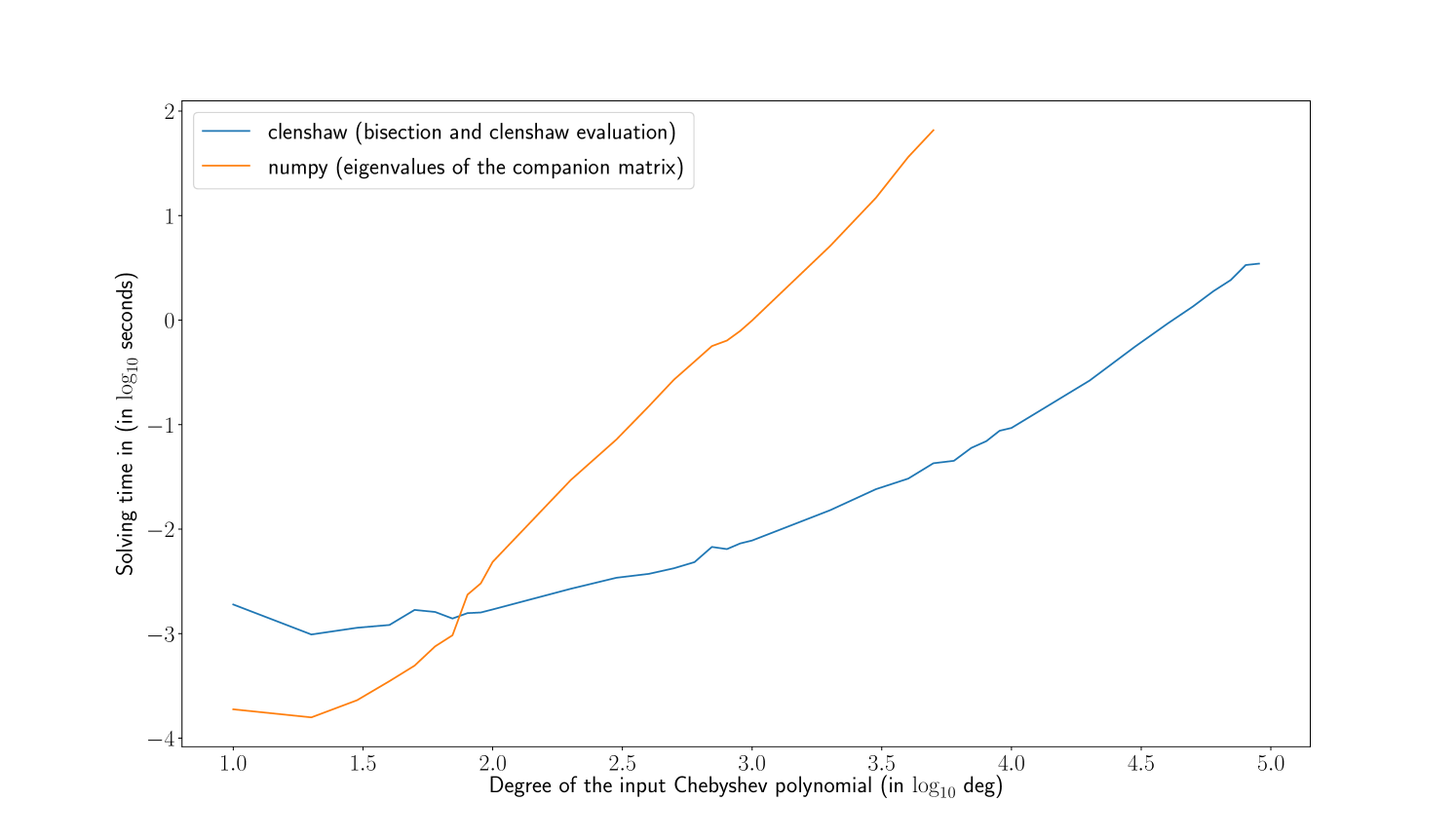
We applied this approach to Chebyshev polynomials whose coefficients are independently and identically distributed with the normal distribution with mean $0$ and variance $1$ .

As illustrated in Figure 1 our code performs significantly better than the classical companion matrix approach. In particular, we could solve polynomials of degree $90000$ in the Chebyshev basis in less than $5$ seconds and polynomials of degree $5000$ in $0.043$ seconds on a quad-core Intel(R) i7-8650U cpu at 1.9GHz. For comparison, the standard numpy function chebroots took more than $65$ seconds for polynomials of degree $5000$ . Moreover, using least square fitting on the ten last values, we observe that our approach has an experimental complexity closer to $\Theta(n^{1.67})$ , whereas the companion matrix approach has a complexity closer to $\Theta(n^{2.39})$ .

Refer to caption — Figure 1: Time for isolating the roots of a random Chebyshev polynomial, on a quad-core Intel(R) i7-8650U cpu at 1.9GHz, with 16G of ram

References

[1] Boyd, J.: Computing zeros on a real interval through chebyshev expansion and polynomial rootfinding. SIAM Journal on Numerical Analysis 40(5), 1666–1682 (2002). https://doi.org/10.1137/S0036142901398325
[2] Boyd, J.: Finding the zeros of a univariate equation: Proxy rootfinders, chebyshev interpolation, and the companion matrix. SIAM Review 55(2), 375–396 (2013). https://doi.org/10.1137/110838297
[3] Elliott, D.: Error analysis of an algorithm for summing certain finite series. Journal of the Australian Mathematical Society 8(2), 213–221 (1968). https://doi.org/10.1017/S1446788700005267
[4] Gentleman, W.M.: An error analysis of Goertzel’s (Watt’s) method for computing Fourier coefficients. The Computer Journal 12(2), 160–164 (01 1969). https://doi.org/10.1093/comjnl/12.2.160
[5] Kobel, A., Rouillier, F., Sagraloff, M.: Computing real roots of real polynomials … and now for real! In: Proceedings of the ACM on International Symposium on Symbolic and Algebraic Computation. pp. 303–310. ISSAC ’16, ACM, New York, NY, USA (2016). https://doi.org/10.1145/2930889.2930937
[6] Moroz, G.: Clenshaw 0.1 (Dec 2019). https://doi.org/10.5281/zenodo.3571248, https://gitlab.inria.fr/gmoro/clenshaw
[7] Oliver, J.: An Error Analysis of the Modified Clenshaw Method for Evaluating Chebyshev and Fourier Series. IMA Journal of Applied Mathematics 20(3), 379–391 (11 1977). https://doi.org/10.1093/imamat/20.3.379