∎
22email: muhammad.qureshi@ucd.ie 33institutetext: Derek Greene 44institutetext: Insight Centre for Data Analytics, University College Dublin, Dublin, Ireland
44email: derek.greene@ucd.ie
EVE: Explainable Vector Based Embedding Technique Using Wikipedia
Abstract
We present an unsupervised explainable word embedding technique, called EVE, which is built upon the structure of Wikipedia. The proposed model defines the dimensions of a semantic vector representing a word using human-readable labels, thereby it readily interpretable. Specifically, each vector is constructed using the Wikipedia category graph structure together with the Wikipedia article link structure. To test the effectiveness of the proposed word embedding model, we consider its usefulness in three fundamental tasks: 1) intruder detection — to evaluate its ability to identify a non-coherent vector from a list of coherent vectors, 2) ability to cluster — to evaluate its tendency to group related vectors together while keeping unrelated vectors in separate clusters, and 3) sorting relevant items first — to evaluate its ability to rank vectors (items) relevant to the query in the top order of the result. For each task, we also propose a strategy to generate a task-specific human-interpretable explanation from the model. These demonstrate the overall effectiveness of the explainable embeddings generated by EVE. Finally, we compare EVE with the Word2Vec, FastText, and GloVe embedding techniques across the three tasks, and report improvements over the state-of-the-art.
Keywords:
Distributional semantics Unsupervised learning Wikipedia1 Introduction
Recently the European Union has approved a regulation which requires that citizens have a “right to explanation” in relation to any algorithmic decision-making (Goodman and Flaxman, 2016). According to this regulation, due to come into force in 2018, an algorithm that makes an automatic decision regarding a user, entitles that user to a clear explanation as to how the decision was made. With this in mind, we present an explainable decision-making approach to generating word embeddings, called the EVE model. Word embeddings reference to a family of techniques that simply describes a concept (i.e. word or phrase) as a vector of real numbers (Pennington et al, 2014). These vectors have been shown useful in a variety of applications, such as topic modelling (Liu et al, 2015), information retrieval (Diaz et al, 2016), and document classification (Kusner et al, 2015)
Generally, word embedding vectors are defined by the context in which those words appear (Baroni et al, 2014). Put simply, “a word is characterized by the company it keeps” (Firth, 1957). To generate these vectors, a number of unsupervised techniques have been proposed which includes applying neural networks (Mikolov et al, 2013a, b; Bojanowski et al, 2016), constructing a co-occurrence matrix followed by dimensionality reduction (Levy and Goldberg, 2014; Pennington et al, 2014), probabilistic models (Globerson et al, 2007; Arora et al, 2016), and explicit representation of words appearing in a context (Levy et al, 2014, 2015).
Existing word embedding techniques do not benefit from the rich semantic information present in structured or semi-structured text. Instead they are trained over a large corpus, such as a Wikipedia dump or collection of news articles, where any structure is ignored. However, in this contribution we propose a model that uses the semantic benefits of structured text for defining embeddings. Moreover, to the best of our knowledge, previous word embedding techniques do not provide human-readable vector dimensions, thus are not readily open to human interpretation. In contrast, EVE associates human-readable semantic labels with each dimension of a vector, thus making it an explainable word embedding technique.
To evaluate EVE, we consider its usefulness in the context of three fundamental tasks that form the basis for many data mining activities – discrimination, clustering, and ranking. We argue for the need for objective evaluation-based strategies to ensure that subjective opinions are discouraged, which may be found tasks such as finding word analogies (Mikolov et al, 2013a). These tasks are applied to seven annotated datasets which differ in terms of topical content and complexity, where we demonstrate not only the ability of EVE to successfully perform these tasks, but also its ability to generate meaningful explanations to support its outputs.
The reminder of the paper is organized as follows. In Section 2, we provide an overview of research relevant to this work. In Section 3, we provide background material covering the structure of Wikipedia, and then describe the methodology of the EVE model in detail. In Section 4, we provide detailed experimental evaluation on the three tasks mentioned above, and also demonstrate the novelty of the EVE model in generating explanations. Finally, in Section 5, we conclude the paper with further discussion and future directions. The relevant dataset and source code for this work can be publicly accessed at http://mlg.ucd.ie/eve.
2 Related Work
Assessing the similarity between words is a fundamental problem in natural language processing (NLP). Research in this area has largely proceeded along two directions: 1) techniques built upon distributional hypothesis whereby contextual information serves as the main source for word representation; 2) techniques built upon knowledge bases whereby encyclopedic knowledge is utilized for determination of word associations. In this section, we provide an overview of these directions, along with a description of some works attempting to bridge the gap between techniques (1) and (2) above through knowledge-powered word embeddings. Finally, we conclude the section with an explanation of the novelty of EVE.
2.1 From Distributional Semantic Models to Word Embeddings
Traditional computational linguistics has shown the utility of contextual information for tasks involving word meanings, in line with the distributional hypothesis which states that “linguistic items with similar distributions have similar meanings” (Harris, 1954). Concretely, distributional semantic models (DSMs) keep count-based vectors corresponding to co-occurring words, followed by a transformation of the vectors via weighting schemes or dimensionality reduction (Baroni and Lenci, 2010; Gallant et al, 1992; Schütze, 1992). A new family of methods, generally known as “word embeddings”, learns word representations in a vector space, where vector weights are set to maximize the probability of the contexts in which the word is observed in the corpus (Bengio et al, 2003; Collobert and Weston, 2008).
A more recent type of word embedding technique word2vec called into question the utility of deep models for learning useful representations, instead proposing continuous bag-of-words (Mikolov et al, 2013a) and skip-gram (Mikolov et al, 2013b) models built upon a simple single-layer architecture. Another recent word embedding technique by Pennington et al (2014) aims to combine best of both strategies, i.e. usage of global corpus statistics available to traditional distributional semantics models and meaningful linear substructures. Finally, Bojanowski et al (2016) proposed an improvement over word2vec by incorporating character n-grams into the model, thereby accounting for sub-word information.
2.2 Knowledge Base Approaches for Semantic Similarity and Relatedness
Another category of work which measures semantic similarity and relatedness between textual units relies on pre-existing knowledge resources (e.g. thesauri, taxonomies or encyclopedias). Within the proposed works in the literature, the key differences lie in the knowledge base employed, the technique used for measurement of semantic distances, and the application domain (Hoffart et al, 2012). Both Budanitsky and Hirst (2006) and Jarmasz (2012) used generalization (‘is a’) relations between words using WordNet-based techniques; Metzler et al (2007) used web search logs for measuring similarity between short texts, and both Strube and Ponzetto (2006) and Gabrilovich and Markovitch (2007) used rich encyclopedic knowledge derived from Wikipedia. Witten and Milne (2008) made use of tf.idf-like measures on Wikipedia links and Yeh et al (2009) made use of random walk algorithm over the graph driven from Wikipedia’s hyperlink structure, infoboxes, and categories. Recently, Jiang et al (2015) utilize various aspects of page organizations within a Wikipedia article to extract Wikipedia-based feature sets for calculating semantic similarity between concepts. Also Qureshi (2015) presented a Wikipedia-based semantic relatedness framework which uses Wikipedia categories and their sub-categories to a certain depth count to define the relatedness between two Wikipedia articles whose categories overlap with the generated hierarchies.
2.3 Knowledge-Powered Word Embeddings
In order to resolve semantic ambiguities associated with text data, researchers have recently attempted to increase the effectiveness of word embeddings by incorporate knowledge bases when learning vector representations for words Xu et al (2014). Two categories of works exist in this direction: 1) encoding entities and relations in a knowledge graph within a vector space with the goal of knowledge base completionBordes et al (2011); Socher et al (2013); 2) enriching the learned vector representations with external knowledge (from within a knowledge base) in order to improve the quality of word embeddings Bian et al (2014). The works in the first category aim to train neural tensor networks for learning a d-dimensional vector for each entity and relation in a given knowledge base. The works in the second category leverage morphological and semantic knowledge from within knowledge bases as an additional input during the process of learning word representations.
The EVE model relates to the works described in Section 2.1 in the sense that these models all attempt to construct word embeddings in order to characterize relatedness between words. However, like the approaches described in Section 2.2, EVE also benefits from semantic information present in structured text, albeit with the different aim of producing word embeddings. The EVE model is different from knowledge-powered word embeddings in that we produce a more general framework by learning vector representations for concepts rather than limiting the model to entities and/or relations. Furthermore, we utilize the structural organization of entities and concepts within a knowledge base to enrich the word vectors. A relevant recent work-in-progress, called ConVec (Sherkat and Milios, 2017), attempts to learn Wikipedia concept embeddings by making use of anchor texts (i.e. linked Wikipedia articles). In contrast, EVE gives a more powerful representation through the combination of Wikipedia categories and articles. Finally, a key characteristic that distinguishes EVE from all existing models is its expressive mode of explanations, as enabled by the use of Wikipedia categories and articles.
3 The EVE Model
3.1 Background on Wikipedia
Before we present the methodology of the proposed EVE model, we firstly provide background information on Wikipedia, whose underlying graph structure forms the basic building blocks of the model.
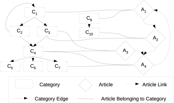
Wikipedia is a multilingual collaboratively-constructed encyclopedia which is actively updated by a large community of volunteer editors. Figure 1 shows the typical Wikipedia graph structure for a set of articles and associated categories. Each article can receive an inlink from another Wikipedia article while it can also outlink to another Wikipedia article. In our example, article A1 receives inlinks from A4 and A1 outlinks to A2. In addition, each article can belong to a number of categories, which are used to group together articles on a similar subject. In Fig. 1, A1 belongs to categories C1 and C9. Furthermore, each Wikipedia category is arranged in a category taxonomy i.e. , each category can have arbitrary number of super-categories and sub-categories. In our case, C5, C6, C7 are sub-categories of C4, whereas C2 and C3 are super-categories of C4.
To motivate with a simple real example, the Wikipedia article “Espresso” receives inlinks from the article “Drink” and it outlinks to the article “Espresso machine”. The article “Espresso” belongs to several categories, including “Coffee drinks” and “Italian cuisine”. The category “Italian cuisine” itself has a number of super-categories (e.g. “Italian culture”, “Cuisine by nationality”) and sub-categories (e.g. “Italian desserts”, “Pizza”). These Wikipedia categories serve as a semantic tag for the articles to which they link (Zesch and Gurevych, 2007).
3.2 Methodology
We now present the methodology for generating word embedding vectors with the EVE model. Firstly, a target word or concept is mapped to a single Wikipedia concept article111This can be an exact match or a partial best match using an information retrieval algorithm. The vector for this concept is then composed of two distinct types of dimensions. The first type quantifies the association of the concept with other Wikipedia articles, while the second type quantifies the association of the concept with Wikipedia categories. The intuition here is that related words or concepts will share both similar article link associations and similar category associations within the Wikipedia graph, while unrelated concepts will differ with respect to both criteria. The methods used to define these associations are explained next.
3.2.1 Vector dimensions related to Wikipedia articles
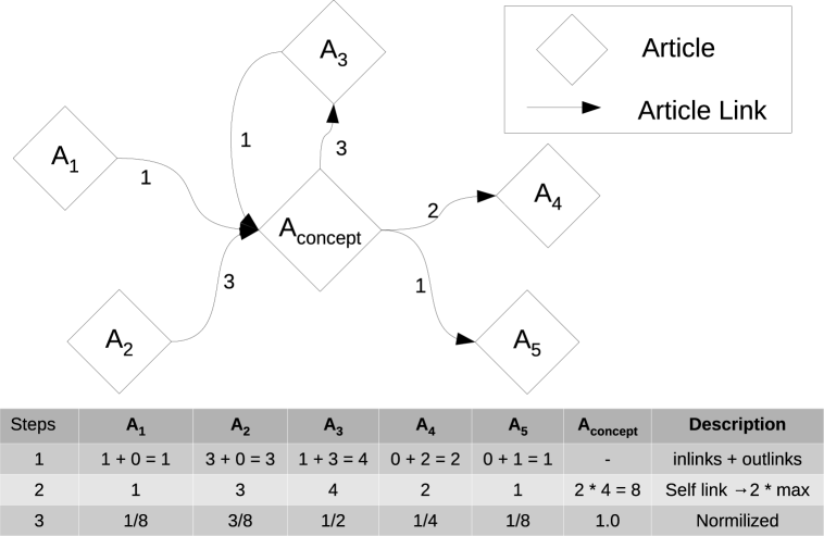
We firstly define the strategy for generating vector dimensions corresponding to individual Wikipedia articles. Given the target concept, which is mapped to a Wikipedia article denoted , we enumerate all incoming links and outgoing links between this article and all other articles. We then create a dimension corresponding to each of those linked articles, where the strength of association for a dimension is defined as the sum of the number of incoming and outgoing links involving an article and . After creating dimensions for all linked articles, we also add a self-link dimension222This dimension the most relevant dimension defining the concept which is the article itself., where the association of with itself is defined to be the twice of the maximum count received from the linking articles.
Fig. 2 shows an example of the strategy. In the first step, all inlinks and outlinks are counted for the other non-concept articles (e.g. has 3 inlinks and 1 outlink from ). In the next step, the self-link score is computed as twice the maximum of sum of inlinks and outlinks from all other articles (which is 8 in this case). In the final step, normalization333In case of best match strategy, where more than one article is mapped to a concept i.e., the score computed is further scaled by the relevance score of the each article for the top-k articles, then reduced by the vector addition, and normalized again. of the scores takes place, dividing by the maximum score (which is 8 in this case). Articles having no links to or from receive a score of 0. Given the sparsity of the Wikipedia link graph, the article-based dimensions are also naturally sparse.
3.2.2 Vector dimensions related to Wikipedia categories
Next we define the method for generating vector dimensions corresponding to all Wikipedia categories which are related to the concept article. The strategy to assign a score to the related Wikipedia categories proceeds as follows:
-
1.
Start by propagating the score uniformly to the categories to which the concept article belongs to (see Fig. 1).
-
2.
A portion of the score is further propagated by the probability of jumping from a category to the categories in the neighborhood.
-
3.
Score propagation continues until a certain hop count is reached (i.e. a threshold value ), or there are no further categories in the neighborhood.
Fig. 3 illustrates the process, where the concept article has a score s, which is 1444In case of the partial best match it is the relevance score returned by BM25 algorithm. for an exact match. First, the score is uniformly propagated across the number of Wikipedia categories and their tree structure to which the article belongs to ( and tree receive from ). In the next step, the directly-related categories ( and ) further propagate the score to their super and sub-categories, while retaining a portion of score. retains a portion by the factor of the score that it propagate to the super and sub-categories. Where is the probability of jumping from a category to either a connected super or sub-category. While retains the full score since there is no super or sub-category for further propagation. In step 3 and onwards, the score continues to propagate in a direction (to either a super or sub-category) until hop count is reached, or until there is no further category to which score could propagate to. In Fig. 3, and are the cases where the score cannot propagate further, while is the stopping condition for the score to propagate when using a threshold .

3.2.3 Overall vector dimensions
Once the sets of dimensions for related Wikipedia articles and categories have been created, we construct an overall vector for the concept article as follows. Eq. 1 shows the vector representation of a concept, where norm is a normalization function, and are the two sets of dimensions, while and are the bias weights which control the importance of the associations with the Wikipedia articles and categories respectively. The bias weights can tuned to give more importance to either type of association. In Eq. 2 we normalize the entire vector such that the sum of the scores of all dimension equates to 1, so that a unit length vector is obtained.
| (1) | |||
| (2) |
The process above is repeated for each word or concept in the input dataset to generate a set of vectors, representing an embedding of the data. In this embedding, each vector dimension is labeled with a tag which corresponds to either a Wikipedia article name or a Wikipedia category name. Therefore, each dimension carries a direct human-interpretable meaning. As we see in the next section, these labeled dimensions prove useful for the generation of algorithmic explanations.
4 Evaluation
In this section we investigate the extent to which embeddings generated using the EVE model are useful in three fundamental data mining tasks. Firstly, we describe a number of alternative baseline methods, along with the relevant parameter settings. Then we describe the dataset which is used for the evaluations, and finally we report the experimental results to showcase the effectiveness of the model. We also highlight the benefits of the explanations generated as part of this process.
4.1 Baselines and Parameters
We compare EVE with three popular word embedding algorithms: Word2Vec, FastText, and GloVe. For Word2Vec and FastText, we trained two well-known variants of each – i.e. the continuous bag of words model (CBOW) and the skip-gram model (SG). For GloVe, we trained the standard model.
For each baseline, we use the default implementation parameter values (window_size=5, vector_dimensions=100), except for the minimum document frequency threshold, which is set to 1 to generate all word vectors, even for rare words. This enables direct comparisons to be made with EVE. For EVE, we use uniform bias weights (i.e. =0.5, =0.5). This provides equal importance to both dimension types. The parameter =0.5 was chosen arbitrarily, so as to retain half of the score by the category while the rest is propagated.
4.2 Dataset
To evaluate the performance of the different models, we constructed a new dataset from the complete 2015 English-language Wikipedia dump, composed of seven different topical types, each containing at least five sub-topical categories. On average each sub-topical category contains a list of 20 items or concepts. The usefulness of the dataset lies in the fact that the organization, from topics to categories to items, is made on the bases of factual position.
| Topical Type | Categories | Mean Items per | Example (Category: Items) |
|---|---|---|---|
| Category | |||
| Animal class | 5 | 20 | Mammal: Baleen whale, Elephant, |
| Primate | |||
| Continent to country | 6 | 17 | Europe: Albania, Belgium, Bulgaria |
| Cuisine | 5 | 20 | Italian cuisine: Agnolotti, Pasta, Pizza |
| European cities | 5 | 20 | Germany: Berlin, Bielefeld, Bonn |
| Movie genres | 5 | 20 | Science fiction film: RoboCop, |
| The Matrix, Westworld | |||
| Music genres | 5 | 20 | Grunge: Alice in Chains |
| Chris Cornell, Eddie Vedder | |||
| Nobel laureates | 5 | 20 | Nobel laureates in Physics: |
| Albert Einstein, Niels Bohr |
| Topical Type | Categories |
|---|---|
| Animal classes | Mammal, Reptile, Bird, Amphibian, Fish |
| Continent to Country | Africa, Europe, Asia, South America, North America, Oceania |
| Cuisine | Italian cuisine, Mexican cuisine, Pakistani cuisine, |
| Swedish cuisine, Vietnamese cuisine | |
| European cities | France, Germany, Great Britain, Italy, Spain |
| Movie genres | Animation, Crime film, Horror film, Science fiction film, |
| Western (genre) | |
| Music genres | Jazz, Classical music, Grunge, Hip hop music, Britpop |
| Nobel laureates | Nobel laureates in Chemistry, Nobel Memorial |
| Prize laureates in Economics, Nobel laureates in Literature, | |
| Nobel Peace Prize laureates, Nobel laureates in Physics |
Table 1 shows a statistical summary of the dataset. In this table, the column “Example (Category, Items)” shows an example of a category name in the “Topical Type”, together with a subset of list of items belonging to that category. For instance, in the first row “Topical Type” is Animal class and Mammal is one of the category belonging to this type, while Baleen whale is an item with in the category of Mammal. Similarly there are other categories of the type Animal class such as Reptile. Table 2 shows the list of categories for each topical type.
All embedding algorithms in our comparison were trained on this dataset. In case of baseline models, we use “article labels”, “article redirects”, “category labels”, and “long abstracts”, with each entry as a separate document. Note that, prior to training, we filter out four non-informative Wikipedia categories which can be viewed as being analogous to stopwords: {“articles contain video clips”, “hidden categories”, “articles created via the article wizard”, “unprintworthy redirects”}.
4.3 Experiments
To compare the EVE model with the various baseline methods, we define three general purpose data mining tasks: intruder detection, ability to cluster, ability to sort relevant items first. In the following sections we define the tasks separately, each accompanied by experimental results and explanations.
4.3.1 Experiment 1: Intruder detection
First we evaluate the performance of EVE when attempting to detect an unrelated “intruder” item from a list of n items, where the rest of the items in the list are semantically related to one another. The ground truth for the correct relations between articles are based on the “topical types” in the dataset.
Task definition:
For a given “topical type”, we randomly choose four items belonging to one category and one intruder item from a different category of the same “topical type”. After repeating this process exhaustively for all combinations for all topical types, we generated 13,532,280 results for this task. Table 3 shows the breakdown of the total number of queries for each of the “topical types”.
Example of a query:
For the “topical type” European cities, we randomly choose four related items from the “category” Great Britain such as London, Birmingham, Manchester, Liverpool, while we randomly choose an intruder item Berlin from the “category” Germany. Each of the models is presented with the five items, where the challenge is to identify Berlin as the intruder – the rest of the items are related to each other as they are cities in Great Britain, while Berlin is a city in Germany.
Strategy:
In order to discover the intruder item, we formulate the problem as a maximization of pairwise similarity across all items, the item receiving the least score is least similar to all other items, and thus identified as the intruder. Formally, for each model we compute
| (3) |
where the function is cosine similarity (Manning et al, 2008), and are the item positions in the list of items, and and are the vectors returned by the model under consideration.
| Topical Types | No. of Queries |
|---|---|
| Animal class | 1,938,000 |
| Continent to country | 1,904,280 |
| Cuisine | 1,938,000 |
| European cities | 1,938,000 |
| Movie genres | 1,938,000 |
| Music genres | 1,938,000 |
| Nobel laureates | 1,938,000 |
| Total | 13,532,280 |
Results:
To evaluate the effectiveness of the EVE model against the baselines for this task, we use (Manning et al, 2008) as the measure for finding the intruder item. Accuracy is defined as the ratio of correct results (or correct number of intruder items) to the total number of results returned by the model:
| (4) |
Table 4 shows the experimental results for the six models in this task. From the table it is evident that the EVE model significantly outperforms rest of the models overall. However, in the case of two “topical types”, the FastText CBOW yields better results. To explain this, we next show explanations generated by the EVE model while making decisions for the intruder detection task.
| EVE | Word2Vec | Word2Vec | FastText | FastText | GloVe | |
|---|---|---|---|---|---|---|
| CBOW | SG | CBOW | SG | |||
| Animal class | 0.77 | 0.39 | 0.42 | 0.36 | 0.43 | 0.31 |
| Continent to Country | 0.75 | 0.70 | 0.76 | 0.79 | 0.79 | 0.73 |
| Cuisine | 0.97 | 0.34 | 0.43 | 0.62 | 0.75 | 0.25 |
| European cities | 0.94 | 0.93 | 0.98 | 0.91 | 0.99 | 0.74 |
| Movie genres | 0.71 | 0.23 | 0.24 | 0.22 | 0.25 | 0.21 |
| Music genres | 0.87 | 0.56 | 0.59 | 0.50 | 0.57 | 0.38 |
| Nobel laureates | 0.91 | 0.28 | 0.28 | 0.23 | 0.27 | 0.24 |
| Average | 0.85 | 0.50 | 0.52 | 0.52 | 0.58 | 0.41 |
-
•
Note: all p-values are for EVE with respect to all baselines
Explanation from the EVE model:
Using the labeled dimensions in vectors produced by EVE, we define the process to generate effective explanations for the intruder detection task in Algorithm 1 as follows. The inputs to this algorithm are the vectors of items, and the intruder item identified by the EVE model. In step 1, we calculate the mean vector of all the vectors. In step 2 and 3, we subtract the influence of intruder and mean of vectors from each other to obtain dominant vector spaces to represent detected coherent items and intruder item respectively. In step 4 and 5, we order the labeled dimensions by their informativeness (i.e. the dimension with the highest score is the most informative dimension). Finally, we return a ranked list of informative vector dimensions for the both non-intruders and the intruder as an explanation for the output of the task.
| Non-Intruder | Intruder |
|---|---|
| falconiformes | turonian first appearances |
| birds of prey | snakes |
| seabirds | squamata |
| ypresian first appearances | predators |
| psittaciformes | lepidosaurs |
| parrots | predation |
| rupelian first appearances | carnivorous animals |
| gulls | venomous snakes |
| bird families | snakes in art |
Table 5 and 6 show sample explanations generated by the EVE model, where the model has detected a correct and incorrect intruder item respectively. In Table 5, the query has items selected from “topical type” animal class, where four of the items belong to the “category” birds, while the item ‘snake’ belongs to the “category” reptile. As can be seen from the table, the bold features in the non-intruder and intruder column obviously represent bird family and snake respectively, which is the correct inference. Furthermore, the non-bold features in the non-intruder and intruder columns represent deeper relevant relations which may require some domain expertise. For instance, falconiformes are a family of 60+ species in the order of birds and turonian is the evolutionary era of the specific genera.
| Non-Intruder | Intruder |
|---|---|
| english-language films | studiocanal films |
| american independent films | splatter films |
| american horror films | final destination films |
| universal pictures films | films shot in vancouver |
| post-apocalyptic films | films shot in toronto |
| films based on science fiction novels | films shot in san francisco, california |
| 2000s science fiction films | films set in new york |
| ghost films | films set in 1999 |
| films shot in los angeles, california | film scores by shirley walker |
In the example in Table 6, the query has items selected from the “topical type” movie genres, where four of the items belong to the “category” horror film, while the intruder item ‘Children of Men’ belongs to the “category” science fiction film. In this example, EVE identifies the wrong intruder item according to the ground truth, recommending instead the item ‘Final Destination (film)’. From the explanation in the table, it becomes clear why the model made this recommendation. We observe that the non-intruder items have a coherent relationship with ‘post-apocalyptic films’ and ‘films based on science fiction novels’ (both ‘I am Legend (film)’ and ‘Children of Men’ belong to these categories). Whereas ‘Final Destination (film)’ was recommended by the model based on features relating to filming location. A key advantage of having an explanation from the model is that it allows us to understand why a mistake occurs and how we might improve the model. In this case, one way to make improvement might be to add a rule filtering Wikipedia categories relating to locations when consider movie genres.
4.3.2 Experiment 2: Ability to cluster
In this experiment, we evaluate the extent to which the distances computed on EVE embeddings can help to group semantically-related items together, while keeping unrelated items apart. This is a fundamental requirement for distance-based methods for cluster analysis.
Task definition:
For all items in a specific “topical type”, we construct an embedding space without using information about the category to which the items belong. The purpose is then to measure the extent to which these items cluster together in the space relative to the ground truth categories. This is done by measuring distances in the space between items that should belong together (i.e. intra-cluster distances) and items that should be kept apart (i.e. inter-cluster distances), as determine by the categories. Since there are seven “topical types”, there are also even queries in this task.
Example of a query:
For the “topical type” Cuisine, we are provided with a list of 100 items in total, where each of the five categories has 20 items. These correspond to cuisine items from five different countries. The idea is to measure the ability of each embedding model to cluster these 100 items back into five categories.
Strategy:
To formally measure the ability of a model to cluster items, we conduct a two-step strategy as follows:
-
1.
Calculate a pairwise similarity matrix between all items of a given “topical type”. The similarity function that we use for this task is the cosine similarity.
-
2.
Transform the similarity matrix to a distance matrix555by simply, 1 - normalized similarity score over each dimension which is used to measure inter and intra-cluster distances relative to the ground truth categories.
Results:
To evaluate the ability to cluster, there are typically two objectives: within-cluster cohesion and between-cluster separation. To this end, we use three well-known cluster validity measures in this task. Firstly, the within-cluster distance (Everitt et al, 2001) is the total of the squared distances between each item and the centroid vector of the cluster to which it has been assigned:
| (5) |
Typically this value is normalized with respect to the number of clusters . The higher the score, the more coherent the clusters. Secondly, the between-cluster distance is the total of the squares of the distances between the each cluster centroid and the centroid of the entire dataset, denoted :
| EVE | Word2Vec | Word2Vec | FastText | FastText | GloVe | |
|---|---|---|---|---|---|---|
| CBOW | SG | CBOW | SG | |||
| Animal class | 2.00 | 13.03 | 6.23 | 10.31 | 7.71 | 12.20 |
| Continent to country | 2.34 | 2.63 | 2.25 | 2.83 | 2.56 | 2.60 |
| Cuisine | 2.92 | 17.31 | 8.88 | 9.74 | 6.25 | 12.36 |
| European cities | 3.13 | 7.72 | 5.46 | 8.30 | 5.75 | 6.86 |
| Movie genres | 6.92 | 11.98 | 6.04 | 9.81 | 5.61 | 17.96 |
| Music genres | 1.90 | 8.25 | 5.25 | 6.72 | 5.77 | 7.72 |
| Nobel laureates | 2.88 | 14.56 | 8.99 | 12.40 | 10.59 | 15.13 |
| Average | 3.16 | 10.78 | 6.16 | 8.59 | 6.32 | 10.69 |
| EVE | Word2Vec | Word2Vec | FastText | FastText | GloVe | |
|---|---|---|---|---|---|---|
| CBOW | SG | CBOW | SG | |||
| Animal class | 0.47 | 1.30 | 0.74 | 1.14 | 1.13 | 0.46 |
| Continent to country | 3.33 | 3.86 | 1.78 | 4.08 | 2.83 | 1.63 |
| Cuisine | 8.18 | 2.12 | 2.12 | 14.52 | 10.80 | 0.88 |
| European cities | 2.39 | 17.14 | 7.45 | 13.24 | 10.86 | 3.84 |
| Movie genres | 1.58 | 0.40 | 0.18 | 0.41 | 0.18 | 0.48 |
| Music genres | 2.23 | 2.79 | 1.60 | 1.16 | 0.18 | 1.68 |
| Nobel laureates | 1.95 | 0.79 | 0.39 | 0.56 | 1.38 | 0.20 |
| Average | 2.88 | 4.06 | 2.04 | 5.02 | 3.96 | 1.31 |
| EVE | Word2Vec | Word2Vec | FastText | FastText | GloVe | |
|---|---|---|---|---|---|---|
| CBOW | SG | CBOW | SG | |||
| Animal class | 7.64 | 5.98 | 4.09 | 3.91 | 4.44 | 5.46 |
| Continent to country | 15.83 | 11.84 | 8.19 | 13.69 | 12.29 | 7.52 |
| Cuisine | 54.18 | 2.38 | 3.51 | 14.25 | 16.00 | 2.23 |
| European cities | 29.08 | 48.57 | 28.98 | 33.73 | 41.88 | 15.53 |
| Movie genres | 12.45 | 1.36 | 1.43 | 1.51 | 1.87 | 1.27 |
| Music genres | 25.04 | 18.01 | 14.80 | 13.06 | 12.93 | 6.09 |
| Nobel laureates | 21.85 | 3.58 | 3.34 | 1.73 | 3.16 | 2.91 |
| Average | 23.72 | 13.10 | 9.19 | 11.70 | 13.22 | 5.86 |
| (6) |
This value is also normalized with respect to the number of clusters . The lower the score, the more well-separated the clusters. Finally, the two above objectives are combined via the CH-Index (Caliński and Harabasz, 1974), using the ratio:
| (7) |
The higher the value of this measure, the better the overall clustering.
From Table 7, we can see that EVE generally performs better than rest of the embedding methods for the within-cluster measure. In Table 8, for the between-cluster measure, EVE is outperformed by FastText CBOW, Word2Vec CBOW, and FastText SG mainly due to the “topical type” Cuisine and European cities where EVE does not perform well. Finally, in Table 9 where the combined aim of clustering is captured through the CH-Index, EVE outperforms the rest of the methods, except in the case of the “topical type” European cities.
Explanation from the EVE model:
Using labeled dimensions from the EVE model, we define a similar strategy for explanation as used in the previous task. However, now instead of discovering an intruder item, the goal is to define categories from items and to define the overall space. Algorithm 2 shows the strategy which requires three inputs: the representing the entire embedding; the list of categories ; the which is the vector space of items belonging to each category. In step 1, we calculate the mean vector representing for the entire space. In step 2, we order the labeled dimensions of the mean vector by the informativeness. In steps 3–6 we iterate over the list of categories (of a “topical type” such as Cuisine) and calculate mean vector for each category’s vector space, which is followed by the ordering of dimensions of the mean vector of category vector space by the informativeness. Finally, we return the most informative features of the entire space and of each category’s vector space.
| Overall | Italian | Mexican | Pakistani | Swedish | Vietnamese |
| space | category | category | category | category | category |
| vietnamese | italian | mexican | pakistani | swedish | vietnamese |
| cuisine | cuisine | cuisine | cuisine | cuisine | cuisine |
| swedish | cuisine | tortilla- | indian | finnish | vietnamese |
| cuisine | of lombardy | based | cuisine | cuisine | words and |
| dishes | phrases | ||||
| mexican | types of | cuisine of | indian | :swedish | : |
| cuisine | pasta | the south- | desserts | cuisine | vietnamese |
| western | cuisine | ||||
| united states | |||||
| italian | pasta | cuisine of | pakistani | desserts | :vietnam |
| cuisine | the western | breads | |||
| united states | |||||
| dumplings | dumplings | :list of | iranian | :sweden | :gànÃÂðáûÃÂng sáúã |
| mexican | breads | ||||
| dishes | |||||
| pakistani | italian- | maize | pakistani | potato | :thit kho |
| cuisine | american | dishes | meat | dishes | tau |
| cuisine | dishes |
Tables 10 and 11 show the explanations generated by the EVE model, in the cases where the model performed best and worse against baselines respectively. In Table 10, the query is the list of items from “topical type” cuisine. As can be seen from the bold entries in the table, the explanation conveys the main idea about both the overall space and the individual categories. For example, in the overall space, we can see the cuisines by different nationalities, and likewise we can see the name of nationality from which the cuisine is originated from (e.g. Italian cuisine for the “Italian category” and Pakistani breads for the “Pakistani category”). As for the non-bold entries, we can also observe relevant features but at a deeper semantic level. For example, cuisine of Lombardy in “Italian category” where Lombardy is a region in Italy, and likewise tortilla-based dishes in the Mexican category where tortilla is a primary ingredient in Mexican cuisine.
| Overall | France | Great | Germany | Italy | Spain |
| space | category | Britain | category | category | category |
| category | |||||
| prefectures | prefectures | articles | university | world | university |
| in france | in france | including | towns in | heritage | towns in |
| recorded | germany | sites in | spain | ||
| pronuncia- | italy | ||||
| tions (uk | |||||
| english) | |||||
| university | port cities | county towns | members | mediterra- | populated |
| towns in | and towns | in england | of the | nean port | coastal |
| germany | on the fren- | hanseatic | cities and | places in | |
| ch atlantic | league | towns in | spain | ||
| coast | italy | ||||
| members | cities in | metropolitan | german | populated | roman |
| of the | france | boroughs | state | coastal | sites in |
| hanseatic | capitals | places in | spain | ||
| league | italy | ||||
| articles | subpre- | university | cities in | cities and | port cities |
| including | fectures | towns in the | north rhine- | towns in | and towns |
| recorded | in france | united | westphalia | emilia | on the |
| pronuncia- | kingdom | romagna | spanish | ||
| tions (uk | atlantic coast | ||||
| english) | coast | ||||
| capitals | world | populated | rhine | former | tourism |
| of former | heritage | places | province | capitals | in spain |
| nations | sites in | established | of italy | ||
| france | in the 1st | ||||
| century | |||||
| german | communes | fortified | populated | capitals | mediterranean |
| state | of nord | settlements | places on | of former | port cities |
| capitals | (french | the rhine | nations | and towns in | |
| department) | spain |
In Table 11, the query is the list of items from “topical type” European cities and this is the example where EVE model performs worse. However, the explanation allows us to understand why this is the case. As can been from the explanation table, the bold features show historic relationships across different countries, such as “capitals of former nations”, “fortified settlements”, and “Roman sites in Spain”. Similarly, it can also be observed in non-bold features such as “former capital of Italy”. Based on this explanation, we could potentially decide to apply a rule that would exclude any historical articles or categories when generating the embedding for this type of task in future.
Visualization:
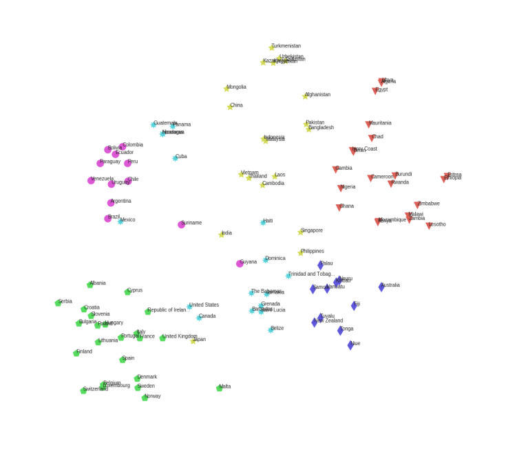
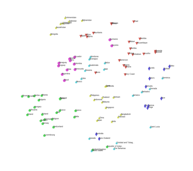
Since scatter plots are often used to represent the output of a cluster analysis process, we generate a visualization of all embeddings using T-SNE (Maaten and Hinton, 2008), which is a tool to visually represent high-dimensional data by reducing it to 2–3 dimensions for presentation.666The full set of experimental visualizations is available at http://mlg.ucd.ie/eve/. For the interest of reader, Fig. 4 shows a visualization generated using EVE and GloVe when the list of items are selected from the “topical type” country to continent. As can be seen from the plot, the ground truth categories exhibit better clustering behavior when using the space from the EVE model, when compared to the Glove model. This is also reflected in the corresponding scores in Tables 7, 8, and 9.
4.3.3 Experiment 3: Sorting relevant items first
Task definition:
The objective of this task is to rank a list of items based on their relevance to a given query item. According to the ground truth associated with our dataset, items which belong to the same ‘category’ of “topical type” as the query should be ranked above items which do not belong that ‘category’ (i.e. they are irrelevant to the query). In this task the total number of queries is equal to the total number of categories in the dataset – i.e. 36 (see table 1).
Example of a query:
Unlike the previous tasks, here ‘category’ is used as a query in this task. For example, for the ‘category’ Nobel laureates in Physics, the task is to sort all items from “topical type” Nobel laureates such that the list of items from ‘category’ Nobel laureates in Physics are ranked ahead of the rest of the items. Thus, Niels Bohr, who is a laureate in Physics, should appear near the top of the ranking, unlike Elihu Root, who is a prize winner in Peace.
Strategy:
In order to sort items relevant to a category, we define a simple two-step strategy as follows:
-
1.
Calculate the cosine similarity between all items and a category belonging to “topical type” in the model space.
-
2.
Sort the list of items in descending order according to their similarity scores with the category.
Based on this strategy, a successful model should rank items with the same ‘category’ before irrelevant items.
Results:
We use precision-at- () and average precision () (Manning et al, 2008) as the measures to evaluate the effectiveness of the sorting ability of each embedding model with respect to relevance of items to a category. captures how many relevant items are calculated at a certain rank (or in the results), while captures how early a relevant item is retrieved on average. It may happen that two models have the same value of , while one of the models retrieves relevant items in an earlier order of rank, thus achieving a higher value. is defined as the ratio of relevant items retrieved in the retrieved items, whereas is the average of values computed after each relevant item is retrieved. Equations 8 and 9 show the formal definitions of both measures.
| (8) |
| (9) | |||
Tables 12 and 13 show the experimental results of the sorting relevant items first task. We choose (), since on average there are 20 items in each category in the dataset. As can be seen from tables, the EVE model generally outperforms the rest of models, except for the “topical type” European cities where it gets outperformed by a factor of 1.05 and 1.09 times in terms of and respectively, while in all other cases EVE outperforms other algorithm by at least 1.51 and 1.37 times in terms of and respectively. On average, the EVE model outperforms the second best algorithm by a factor of 1.8 and 1.67 times in terms of and respectively. In the next section, we show the corresponding explanations generated by the EVE model for this task.
| EVE | Word2Vec | Word2Vec | FastText | FastText | GloVe | |
|---|---|---|---|---|---|---|
| CBOW | SG | CBOW | SG | |||
| Animal class | 0.72 | 0.34 | 0.38 | 0.41 | 0.47 | 0.22 |
| Continent to country | 0.95 | 0.54 | 0.51 | 0.63 | 0.59 | 0.31 |
| Cuisine | 0.97 | 0.36 | 0.49 | 0.54 | 0.54 | 0.24 |
| European cities | 0.91 | 0.85 | 0.91 | 0.86 | 0.96 | 0.61 |
| Movie genres | 0.87 | 0.30 | 0.31 | 0.24 | 0.29 | 0.24 |
| Music genres | 0.90 | 0.33 | 0.30 | 0.28 | 0.37 | 0.21 |
| Nobel laureates | 0.99 | 0.27 | 0.22 | 0.20 | 0.25 | 0.20 |
| Average | 0.90 | 0.43 | 0.45 | 0.45 | 0.50 | 0.29 |
| EVE | Word2Vec | Word2Vec | FastText | FastText | GloVe | |
|---|---|---|---|---|---|---|
| CBOW | SG | CBOW | SG | |||
| Animal class | 0.72 | 0.38 | 0.42 | 0.45 | 0.52 | 0.27 |
| Continent to country | 0.92 | 0.55 | 0.54 | 0.65 | 0.67 | 0.33 |
| Cuisine | 0.99 | 0.39 | 0.58 | 0.59 | 0.59 | 0.27 |
| European cities | 0.91 | 0.91 | 0.97 | 0.93 | 0.99 | 0.65 |
| Movie genres | 0.88 | 0.32 | 0.35 | 0.29 | 0.34 | 0.29 |
| Music genres | 0.91 | 0.35 | 0.34 | 0.33 | 0.40 | 0.29 |
| Nobel laureates | 1.00 | 0.26 | 0.26 | 0.24 | 0.29 | 0.24 |
| Average | 0.90 | 0.45 | 0.49 | 0.49 | 0.54 | 0.33 |
Explanation from the EVE model:
Using the labeled dimensions provided by the EVE model, we define a strategy for generating explanations for the sorting relevant items first task in Algorithm 3. The strategy requires three inputs. The first is the which is composed of category vector and item vectors. The second input is the which is a column matrix, composed of similarity score between the category vector with itself and item vectors. In this matrix the first entry is 1.0 because of the self similarity of the category vector. The final input is a list of items . In the step 1 and 2, a weighted mean vector of space is calculated, where the weights are the similarity scores between the vectors in the space and the category vector. In steps 3–6, we iterate over the list of items and calculate the product between the weighted mean vector of the space and the item vector. After taking the product, we order the dimensions by the informativeness. Finally, we return the ranked list of informative features for each item.
Tables 14 and 15 show sample explanations generated by the EVE model. For illustration purposes we select the “topical types” Nobel laureates and Music genres for explanations, as these are the only remaining “topical types” which we have not looked at so far in the other tasks.
| Kurt Alder (Chemistry) | Linus Pauling (Peace) |
| First correct found at #1 | First incorrect found at #20 |
| nobel laureates in chemistry | nobel laureates in chemistry |
| german nobel laureates | Guggenheim fellows |
| organic chemists | american nobel laureates |
| university of kiel faculty | national medal of science laureates |
| university of kiel alumni | american physical chemists |
| university of cologne faculty | american people of scottish descent |
In Table 14, the query is ‘category’ Nobel laureates in Chemistry from the “topical type” nobel laureates. We show the informative features for two cases – the first correct result which appears at rank 1 in the sorted lists produced by EVE, and the first incorrect result which appears at rank 20. The bold features indicates that both individuals are Nobel laureates in Chemistry. However, Linus Pauling also appears to be associated with the Peace category. This reflects that fact that, in fact, Linus Pauling is a two time Nobel laureate in two different categories, Chemistry and Peace. While generating the dataset used in our evaluations, the annotators randomly selected items to belong to a category from the full set of available items, without taking into account occasional cases where an item may belong into two categories. This case highlights the fact that EVE explanations are meaningful and can inform the choices made by human annotators.
| Ludwig van Beethoven (Classical) | Herbie Hancock (Jazz) |
|---|---|
| First correct found at #1 | First incorrect found at #18 |
| romantic composers | 20th-century american musicians |
| 19th-century classical composers | :classical music |
| composers for piano | american jazz composers |
| german male classical composers | grammy award winners |
| german classical composers | :herbie hancock |
| 19th-century german people | american jazz bandleaders |
In Table 15, the query is ‘category’ Classical music from the “topical type” music genres. We see that the first correct result is observed at rank 1 and the first incorrect result is at rank 18. The bold features show that both individuals are associated with classical music. Looking at the biography of the musician Herbie Hancock more closely, we find that he received an education in classical music and he is also well known in the classical genre, although not as strongly as he is known for Jazz music. This again goes to show that explanations generated using the EVE model are insightful and can support the activity of manual annotators.
5 Conclusion and Future Directions
In this contribution, we presented a novel technique, EVE, for generating vector representations of words using information from Wikipedia. This work represents a first step in the direction of explainable word embeddings, where the core of this interpretability lies in the use of labeled vector dimensions corresponding to either Wikipedia categories or Wikipedia articles. We have demonstrated that, not only are the resulting embeddings useful for fundamental data mining tasks, but the provision of labeled dimensions readily supports the generation of task-specific explanations via simple vector operations. We do not argue that embeddings generated on structured data, such as those produced by the EVE model, would replace the prevalent existing word embedding models. Rather, we have shown that using structured data can provide additional benefits beyond those afforded by existing approaches. An interesting aspect to consider in future would be the use of hybrid models, generated on both structured data and unstructured text, which could still retain aspects of explanations as proposed in this work.
In future, we would like to investigate the effect of the popularity of a word or concept (i.e. the number of non-zero dimensions in the embedding). For example, a cuisine-related item might have fewer non-zero dimensions when compared to a country-related item. Similarly, an interesting direction might be to analyze embedding spaces and sub-spaces to learn more about correlations of dimensions, while addressing a task or the effects of dimensionality reduction (even though spaces may be sparse). Another interesting avenue for future work could be to explore different ways of generating task-specific explanations, and to investigate how these explanations might be presented effectively to a user.
Acknowledgements. This publication has emanated from research conducted with the support of Science Foundation Ireland (SFI), under Grant Number SFI/12/ RC/2289.
References
- Arora et al (2016) Arora S, Li Y, Liang Y, Ma T, Risteski A (2016) A latent variable model approach to pmi-based word embeddings. Tr Assoc Computational Linguistics 4:385–399
- Baroni and Lenci (2010) Baroni M, Lenci A (2010) Distributional memory: A general framework for corpus-based semantics. Computational Linguistics 36(4):673–721
- Baroni et al (2014) Baroni M, Dinu G, Kruszewski G (2014) Don’t count, predict! a systematic comparison of context-counting vs. context-predicting semantic vectors. In: ACL (1), pp 238–247
- Bengio et al (2003) Bengio Y, Ducharme R, Vincent P, Jauvin C (2003) A neural probabilistic language model. JMLR 3(Feb):1137–1155
- Bian et al (2014) Bian J, Gao B, Liu TY (2014) Knowledge-powered deep learning for word embedding. In: Joint European Conference on Machine Learning and Knowledge Discovery in Databases, Springer, pp 132–148
- Bojanowski et al (2016) Bojanowski P, Grave E, Joulin A, Mikolov T (2016) Enriching word vectors with subword information. arXiv preprint arXiv:160704606
- Bordes et al (2011) Bordes A, Weston J, Collobert R, Bengio Y (2011) Learning structured embeddings of knowledge bases. In: Conference on artificial intelligence, EPFL-CONF-192344
- Budanitsky and Hirst (2006) Budanitsky A, Hirst G (2006) Evaluating wordnet-based measures of lexical semantic relatedness. Computational Linguistics 32(1):13–47
- Caliński and Harabasz (1974) Caliński T, Harabasz J (1974) A dendrite method for cluster analysis. Communications in Statistics-theory and Methods 3(1):1–27
- Collobert and Weston (2008) Collobert R, Weston J (2008) A unified architecture for natural language processing: Deep neural networks with multitask learning. In: Proc. ICML’2008, ACM, pp 160–167
- Diaz et al (2016) Diaz F, Mitra B, Craswell N (2016) Query expansion with locally-trained word embeddings. arXiv preprint arXiv:160507891
- Everitt et al (2001) Everitt B, Landau S, Leese M (2001) Cluster Analysis. Hodder Arnold Publication, Wiley
- Firth (1957) Firth J (1957) A synopsis of linguistic theory 1930-1955. Studies in linguistic analysis pp 1–32
- Gabrilovich and Markovitch (2007) Gabrilovich E, Markovitch S (2007) Computing semantic relatedness using wikipedia-based explicit semantic analysis. In: Proc. IJCAI’07, vol 7, pp 1606–1611
- Gallant et al (1992) Gallant SI, Caid WR, Carleton J, Hecht-Nielsen R, Qing KP, Sudbeck D (1992) Hnc’s matchplus system. In: ACM SIGIR Forum, ACM, vol 26, pp 34–38
- Globerson et al (2007) Globerson A, Chechik G, Pereira F, Tishby N (2007) Euclidean embedding of co-occurrence data. JMLR 8(Oct):2265–2295
- Goodman and Flaxman (2016) Goodman B, Flaxman S (2016) European union regulations on algorithmic decision-making and a” right to explanation”. arXiv preprint arXiv:160608813
- Harris (1954) Harris ZS (1954) Distributional structure. Word 10(2-3):146–162
- Hoffart et al (2012) Hoffart J, Seufert S, Nguyen DB, Theobald M, Weikum G (2012) Kore: Keyphrase overlap relatedness for entity disambiguation. In: Proc. 21st ACM International Conference on Information and Knowledge Management, pp 545–554
- Jarmasz (2012) Jarmasz M (2012) Roget’s thesaurus as a lexical resource for natural language processing. arXiv preprint arXiv:12040140
- Jiang et al (2015) Jiang Y, Zhang X, Tang Y, Nie R (2015) Feature-based approaches to semantic similarity assessment of concepts using wikipedia. Info Processing & Management 51(3):215–234
- Kusner et al (2015) Kusner MJ, Sun Y, Kolkin NI, Weinberger KQ (2015) From word embeddings to document distances. In: Proc. ICML’2015, pp 957–966
- Levy and Goldberg (2014) Levy O, Goldberg Y (2014) Neural word embedding as implicit matrix factorization. In: Proc. NIPS’2014, pp 2177–2185
- Levy et al (2014) Levy O, Goldberg Y, Ramat-Gan I (2014) Linguistic regularities in sparse and explicit word representations. In: CoNLL, pp 171–180
- Levy et al (2015) Levy O, Goldberg Y, Dagan I (2015) Improving distributional similarity with lessons learned from word embeddings. Tr Assoc Computational Linguistics 3:211–225
- Liu et al (2015) Liu Y, Liu Z, Chua TS, Sun M (2015) Topical word embeddings. In: AAAI, pp 2418–2424
- Maaten and Hinton (2008) Maaten Lvd, Hinton G (2008) Visualizing data using t-sne. JMLR 9(Nov):2579–2605
- Manning et al (2008) Manning CD, Raghavan P, Schütze H (2008) Introduction to Information Retrieval. Cambridge University Press, New York, NY, USA
- Metzler et al (2007) Metzler D, Dumais S, Meek C (2007) Similarity measures for short segments of text. In: European Conference on Information Retrieval, Springer, pp 16–27
- Mikolov et al (2013a) Mikolov T, Chen K, Corrado G, Dean J (2013a) Efficient estimation of word representations in vector space. arXiv preprint arXiv:13013781
- Mikolov et al (2013b) Mikolov T, Sutskever I, Chen K, Corrado GS, Dean J (2013b) Distributed representations of words and phrases and their compositionality. In: Proc. NIPS’2013, pp 3111–3119
- Pennington et al (2014) Pennington J, Socher R, Manning CD (2014) Glove: Global vectors for word representation. In: Empirical Methods in Natural Language Processing (EMNLP), pp 1532–1543
- Qureshi (2015) Qureshi MA (2015) Utilising wikipedia for text mining applications. PhD thesis, National University of Ireland Galway
- Schütze (1992) Schütze H (1992) Word space. In: Proc. NIPS’1992, pp 895–902
- Sherkat and Milios (2017) Sherkat E, Milios E (2017) Vector embedding of wikipedia concepts and entities. arXiv preprint arXiv:170203470
- Socher et al (2013) Socher R, Chen D, Manning CD, Ng A (2013) Reasoning with neural tensor networks for knowledge base completion. In: Proc. NIPS’2013, pp 926–934
- Strube and Ponzetto (2006) Strube M, Ponzetto SP (2006) Wikirelate! computing semantic relatedness using wikipedia. In: Proc. 21st national conference on Artificial intelligence, pp 1419–1424
- Witten and Milne (2008) Witten I, Milne D (2008) An effective, low-cost measure of semantic relatedness obtained from wikipedia links. In: AAAI Workshop on Wikipedia and Artificial Intelligence: an Evolving Synergy, pp 25–30
- Xu et al (2014) Xu C, Bai Y, Bian J, Gao B, Wang G, Liu X, Liu TY (2014) Rc-net: A general framework for incorporating knowledge into word representations. In: Proc. 23rd ACM International Conference on Conference on Information and Knowledge Management, pp 1219–1228
- Yeh et al (2009) Yeh E, Ramage D, Manning CD, Agirre E, Soroa A (2009) Wikiwalk: random walks on wikipedia for semantic relatedness. In: Proc. 2009 Workshop on Graph-based Methods for Natural Language Processing, pp 41–49
- Zesch and Gurevych (2007) Zesch T, Gurevych I (2007) Analysis of the wikipedia category graph for nlp applications. In: Proc. TextGraphs-2 Workshop (NAACL-HLT 2007), pp 1–8