This paper was converted on www.awesomepapers.org from LaTeX by an anonymous user.
Want to know more? Visit the Converter page.

Event-Triggered Active Disturbance Rejection Control for Uncertain Random Nonlinear Systems

Ze-Hao Wu zehaowu@amss.ac.cn    Feiqi Deng aufqdeng@scut.edu.cn    Pengyu Zeng pyzeng@outlook.com    Hua-Cheng Zhou hczhou@amss.ac.cn    Hongyi Li lihongyi2009@swu.edu.cn School of Mathematics and Big Data, Foshan University, Foshan 528000, China Systems Engineering Institute, South China University of Technology, Guangzhou 510640, China School of Mathematics and Statistics, HNP-LAMA, Central South University, Changsha 410075, China School of Electronic and Information Engineering and Chongqing Key Laboratory of Generic Technology and System of Service Robots, Southwest University, Chongqing 400715, China
Abstract

In this paper, event-triggered active disturbance rejection control (ADRC) is first addressed for a class of uncertain random nonlinear systems driven by bounded noise and colored noise. The event-triggered extended state observer (ESO) and ADRC controller are designed, where two respective event-triggering mechanisms with a fixed positive lower bound for the inter-execution times are proposed. The random total disturbance representing the coupling of nonlinear unmodeled dynamics, external deterministic disturbance, bounded noise, and colored noise is estimated in real time by the event-triggered ESO and compensated in the event-triggered feedback loop. Both the mean square and almost surely practical convergence of the closed-loop systems is shown with rigorous theoretical analysis. Finally, some numerical simulations are implemented to validate the proposed control scheme and theoretical results.

keywords:
Random systems; Active disturbance rejection control; Event-triggering mechanisms; Extended state observer.

, , , ,

1 Introduction

Disturbance rejection for uncertain systems has been attracting increasing attention in the past decades since disturbances and uncertainties are widespread in engineering applications. Active disturbance rejection control (ADRC) is a novel control technology based on estimation/compensation strategy, proposed by Han in the late 1980s [9]. The key component of ADRC scheme is extended state observer (ESO), which aims at estimating in real time not only unmeasurable states but also total disturbance representing total effects of internal uncertainties and external disturbances. Based on the estimates obtained via ESO, the ADRC controller composed of a feedback controller and a compensator is devised to achieve disturbance rejection and desired control objective for the plant, where the total disturbance is promptly estimated and compensated in the closed-loop. Since ADRC is proposed, it has been applied in extensive engineering technology applications like general purpose control chips manufactured by Texas Instruments [28], DC-DC power converter [22], permanent magnet synchronous motor [24], Delta robot control [2], and power plant [25], etc.

On the one hand, over the past twenty years much progress on the theoretical foundation of ADRC for uncertain systems has been made including the convergence analysis of ESO and ADRC’s closed-loop, which can be found in the convergence analysis of ESO for a class of uncertain nonlinear systems in [7], the convergence analysis of ADRC’s closed-loop of uncertain random systems in [6], and more all-round designs and theoretical analysis of ADRC for uncertain nonlinear systems in the monographs [8, 26] and the references therein. On the other hand, networked control systems (NCSs), where sensors, actuators, and controllers are spatially distributed, transmit data over a communication network with superiority in reducing installation costs, obtaining higher dependability, and improving system flexibility, and then have been applied extensively. It is important to note that the bandwidth of the wireless sensor-actuator networks and computation resources are limited in NCSs. Event-triggering mechanisms (ETMs) have been widely applied in improving communication efficiency for NCSs with ensuring control quality, see, e.g., [10, 30, 1, 4, 21] and the references therein. The ESO designs via the continuously transmitted output measurement and the ADRC controller designs based on continuous-time estimates obtained by ESO like those in aforementioned literature may become impracticable for uncertain systems in networked environment. This further promotes the recent development of event-triggered ADRC for uncertain systems, see, e.g., [27, 11, 23] and the references therein. In the framework of event-triggered control, information transmission and control signal renovating occur only when essential for the system, leading to momentous efficiency in saving communication/computation resources.

It is widely acknowledged that disturbances and uncertainties are more likely to be of random characteristic in engineering applications. Many important developments have been made in the feedback control of stochastic systems driven by white noise described by stochastic differential equations (SDEs) in the past few decades, see for instance [3, 29]. Recently, event-triggered control for stochastic systems has also been drawing great attention, see, e.g., [16, 17, 18, 19]. However, the mean power of white noise is infinite so that SDE is not always appropriate for describing many practical systems, especially those in engineering [33]. Random differential equations (RDEs) have been widely used as the dynamic models, which are driven by second moment processes whose mean power is bounded, see, e.g., [13, 14]. It was not until 2014 that the existence and uniqueness of solutions and stability analysis of RDEs were developed in [31]. A series of relevant advancements occurred subsequently, see e.g., [33, 35, 36]. For example, the trajectory tracking control for Lagrange systems driven by second moment processes was addressed in [33]; The existence and uniqueness of the global solution, stability, and the adaptive output feedback regulation control design for random nonlinear time-delay systems were investigated in [35]; The event-triggered adaptive tracking control for RDE systems with coexisting parametric uncertainties and severe nonlinearities was addressed in [36]. More research progresses on random systems in the field of control can be found in the recent review paper [34]. Recently, linear and nonlinear event-triggered ESOs have been designed for the open-loop of a class of uncertain random nonlinear systems driven by bounded noise and colored noise which are representative second moment processes, and the mean square and almost sure convergence of proposed ESOs have been presented with rigorous theoretical analysis [32].

A prominent element for the ETM-based observer and controller to be workable is to prevent the Zeno phenomenon (i.e., the triggering conditions are satisfied infinite times in finite time). This leads to enormous difficulty in developing event-triggered control for stochastic/random systems, because the execution/sampling times and the inter-execution times are both random and then a positive constant lower bound for the random inter-execution times is difficult or even impossible to be obtained. In aforementioned literature like [16, 17, 18, 19], novel ETM with dwell time (time-regularization) or periodic ETM was designed, with the Zeno phenomenon be directly excluded but the theoretical analysis be much more sophisticated.

In this paper, we develop the event-triggered ADRC controller design and convergence analysis for a class of uncertain random nonlinear systems. The main contribution and novelty can be summed up as follows: a) The controlled random nonlinear systems are subject to broad scale random total disturbance involving the coupling of nonlinear unmodeled dynamics, external deterministic disturbance, bounded noise, and colored noise; b) The event-triggered ADRC controller is designed with two feasible event-triggering mechanisms be proposed; c) Both the mean square and almost surely practical convergence of the ADRC’s closed-loop of the uncertain random nonlinear systems is presented with rigorous theoretical proofs.

This paper has the following structure. In Section 2, the problem is formulated, and some preliminaries are introduced. In Section 3, the event-triggered ADRC controller is designed and the main results are presented. The theoretical proofs of main results are given in Section 4. In Section 5, some numerical simulations are carried out to validate the theoretical results, followed up with concluding remarks in Section 6.

2 Problem formulation and preliminaries

Throughout the paper, the following notations are used. 𝔼\mathbb{E} denotes the mathematical expectation; |Z||Z| stands for the absolute value of a scalar ZZ, and Z\|Z\| denotes the 2-norm (or Euclidean norm) of a vector ZZ; 𝕀n\mathbb{I}_{n} denotes the nn-dimensional identity matrix; x¯i(x1,,xi)\bar{x}_{i}\triangleq(x_{1},\cdots,x_{i}), x¯^i(x^1,,x^i)\hat{\bar{x}}_{i}\triangleq(\hat{x}_{1},\cdots,\hat{x}_{i}), x^=x¯^n+1\hat{x}=\hat{\bar{x}}_{n+1}; λmin(Z)\lambda_{\min}(Z) and λmax(Z)\lambda_{\max}(Z) denote the minimum eigenvalue and maximum eigenvalue of a positive definite matrix ZZ; 𝕀Ω\mathbb{I}_{\Omega_{*}} denotes an indicator function with the function value be 11 in the domain Ω\Omega_{*} and be 0 otherwise; (Ω,,𝔽,P)(\Omega,\mathcal{F},\mathbb{F},P) represents a complete filtered probability space with a filtration 𝔽={t}t0\mathbb{F}=\{\mathcal{F}_{t}\}_{t\geq 0}, where two mutually independent one-dimensional standard Brownian motions Bi(t)(i=1,2)B_{i}(t)\;(i=1,2) are defined.

In this paper, the event-triggered ADRC approach is addressed for the output-feedback stabilization and disturbance rejection for a class of uncertain random nonlinear systems driven by bounded noise and colored noise as follows:

{x˙1(t)=x2(t)+g1(x1(t)),x˙2(t)=x3(t)+g2(x1(t),x2(t)),x˙n(t)=f(t,x(t),w1(t),w2(t))+gn(x(t))+u(t),y(t)=x1(t),\left\{\begin{array}[]{l}\dot{x}_{1}(t)=x_{2}(t)+g_{1}(x_{1}(t)),\cr\dot{x}_{2}(t)=x_{3}(t)+g_{2}(x_{1}(t),x_{2}(t)),\cr\hskip 34.14322pt\vdots\cr\dot{x}_{n}(t)=f(t,x(t),w_{1}(t),w_{2}(t))+g_{n}(x(t))+u(t),\cr y(t)=x_{1}(t),\end{array}\right. (1)

where x(t)=(x1(t),,xn(t))nx(t)=(x_{1}(t),\cdots,x_{n}(t))\in\mathbb{R}^{n}, u(t)u(t)\in\mathbb{R}, and y(t)y(t)\in\mathbb{R} are the state, control input, and output measurement of system, respectively; f:[0,)×n+2f:[0,\infty)\times\mathbb{R}^{n+2}\rightarrow\mathbb{R} is an unknown system function, and gi:i(i=1,,n)g_{i}:\mathbb{R}^{i}\rightarrow\mathbb{R}\;(i=1,\cdots,n) are the known ones, but gi(x¯i(t))(i=2,,n)g_{i}(\bar{x}_{i}(t))\;(i=2,\cdots,n) still indicate unknown dynamics because of the unmeasurable state; w1(t)ψ(t,B1(t))w_{1}(t)\triangleq\psi(t,B_{1}(t)) defined by an unknown function ψ:[0,)×\psi:[0,\infty)\times\mathbb{R}\rightarrow\mathbb{R} satisfying Assumption (A2) is the bounded noise, and w2(t)w_{2}(t) is the colored noise that is the solution to the Itô-type stochastic differential equation (see, e.g., [15, p.426], [20, p.101]):

dw2(t)=ρ1w2(t)dt+ρ12ρ2dB2(t),dw_{2}(t)=-\rho_{1}w_{2}(t)dt+\rho_{1}\sqrt{2\rho_{2}}dB_{2}(t), (2)

where ρ1>0\rho_{1}>0 and ρ2>0\rho_{2}>0 are constants representing the correlation time and the noise intensity, respectively, and the initial values w2(0)w_{2}(0)\in\mathbb{R}. ρ1\rho_{1}, ρ2\rho_{2} could be unknown but within known bounded intervals.

The significance of considering these two kinds of random noises can be expounded as follows. It is known that white noise can be a characterization of random disturbances in practice, which is generally understood as a stationary process with zero mean and constant power spectral density. However, white noise is not always workable in characterizing noise in many engineering applications because the mean power of continuous-time white noise is infinite and it has a correlation time of 0 [33]. The colored noise described by (2) is a second moment process, which is with uneven power spectral density and bounded mean power. Compared to white noise, colored noise could be more realistic in describing noise when the real processes have finite or even long correlation time and bounded mean power [15, 33]. More explanations and comparisons of white noise and colored noise and physical backgrounds of colored noise can be found in [14, 15, 31, 33, 34], etc. As for the bounded noise, conventional deterministic disturbance is its special example by letting w1(t)=ψ(t)w_{1}(t)=\psi(t) which is the function with regard to the time argument only, and frequently occurring bounded noises like sin(t+B1(t))\sin(t+B_{1}(t)) and cos(t+B1(t))\cos(t+B_{1}(t)) in practice ([12]) are the concerned ones satisfying the following Assumption (A2).

It was shown in [5] that any uniform observable affine single-input single-output (SISO) nonlinear system can be transformed into the lower triangular form (1) with wi(t)0(i=1,2)w_{i}(t)\equiv 0\;(i=1,2). Moreover, system (1) covers the essential-integral-chain system with matched disturbance and uncertainty as a special case of gi()=0(i=1,,n)g_{i}(\cdot)=0\;(i=1,\cdots,n), which is the normalized form to demonstrate the designing process and applications of ADRC. Numerous engineering systems can be described by system (1) like aforementioned dynamics of DC-DC power converter [22], permanent magnet synchronous motor [24], and Delta robot [2], etc.

It should be pointed out that the convergence of ESO for the open-loop systems in [32] doesn’t directly indicates the convergence of ESO and stability of controlled systems in the ADRC’s closed-loop. This is because in the proof of convergence of estimation error of the random total disturbance including system state for the open-loop systems, the state should be assumed to be bounded in a statistical sense beforehand, while the boundedness of the closed-loop state depends on the convergence of ESO conversely. The boundedness assumption of state for the open-loop systems can be regarded as a slowly varying condition besides the common structural one (like exact observability). This presupposition is unwanted when the ADRC controller is designed, which is not an easy theoretical task. In addition, both the designs and theoretical analysis of this paper are largely distinguished from the deterministic counterpart in [27, 11, 23].

3 Event-triggered ADRC design and main results

Define

xn+1(t)f(t,x(t),w1(t),w2(t)),\displaystyle x_{n+1}(t)\triangleq f(t,x(t),w_{1}(t),w_{2}(t)), (3)

which is a random total disturbance (extended state) involving the nonlinear coupling effects of the nonlinear unmodeled dynamics, external deterministic disturbance, bounded noise, and colored noise. To estimate both unmeasurable state and random total disturbance, the event-triggered ESO is designed via the output and input of system (1) as follows:

{x^˙1(t)=x^2(t)+λ1r(y(tk)x^1(t))+g1(x^1(t)),x^˙2(t)=x^3(t)+λ2r2(y(tk)x^1(t))+g2(x^1(t),x^2(t)),x^˙n(t)=x^n+1(t)+λnrn(y(tk)x^1(t))+gn(x¯^n(t))+u(t),x^˙n+1(t)=λn+1rn+1(y(tk)x^1(t)),t[tk,tk+1),\left\{\begin{array}[]{l}\dot{\hat{x}}_{1}(t)=\hat{x}_{2}(t)+\lambda_{1}r\left(y(t_{k})-\hat{x}_{1}(t)\right)+g_{1}(\hat{x}_{1}(t)),\cr\vskip 0.0pt\cr\dot{\hat{x}}_{2}(t)=\hat{x}_{3}(t)+\lambda_{2}r^{2}\left(y(t_{k})-\hat{x}_{1}(t)\right)+g_{2}(\hat{x}_{1}(t),\hat{x}_{2}(t)),\cr\vskip 0.0pt\cr\hskip 34.14322pt\vdots\cr\vskip 0.0pt\cr\dot{\hat{x}}_{n}(t)=\hat{x}_{n+1}(t)+\lambda_{n}r^{n}\left(y(t_{k})-\hat{x}_{1}(t)\right)+g_{n}(\hat{\bar{x}}_{n}(t))\cr\hskip 34.14322pt+u(t),\cr\vskip 0.0pt\cr\dot{\hat{x}}_{n+1}(t)=\lambda_{n+1}r^{n+1}\left(y(t_{k})-\hat{x}_{1}(t)\right),\;t\in[t_{k},t_{k+1}),\end{array}\right. (4)

where k+k\in\mathbb{Z}^{+}, t1=0t_{1}=0, x^i(t)(i=1,,n+1)\hat{x}_{i}(t)\;(i=1,\cdots,n+1) are the estimates of xi(t)x_{i}(t), rr is the tuning gain, parameters λi(i=1,,n+1)\lambda_{i}\;(i=1,\cdots,n+1) are selected to guarantee that the matrix

H=(λ1100λ2010λn001λn+1000)(n+1)×(n+1)\displaystyle H=\begin{pmatrix}-\lambda_{1}&1&0&\cdots&0\cr-\lambda_{2}&0&1&\cdots&0\cr\cdots&\cdots&\cdots&\cdots&\cdots\cr-\lambda_{n}&0&0&\ddots&1\cr-\lambda_{n+1}&0&0&\cdots&0\end{pmatrix}_{(n+1)\times(n+1)} (5)

is Hurwitz, and tk(k+)t_{k}\;(k\in\mathbb{Z}^{+}) are random execution times (stopping times) determined by the following event-triggering ETM

tk+1=inf{ttk+τ:|y(t)y(tk)|κ1r(n+12)},t_{k+1}=\inf\{t\geq t_{k}+\tau:\;|y(t)-y(t_{k})|\geq\kappa_{1}r^{-(n+\frac{1}{2})}\}, (6)

with τ=ϵ1r(2n+32)\tau=\epsilon_{1}r^{-(2n+\frac{3}{2})} and ϵ1\epsilon_{1}, κ1\kappa_{1} be free positive tuning parameters. For any fixed t[0,)t\in[0,\infty), the last execution time of the ETM (6) before tt can be expressed as follows:

ζt=max{tk:tkt,k+}.\displaystyle\zeta_{t}=\max\{t_{k}:t_{k}\leq t,k\in\mathbb{Z}^{+}\}. (7)

Therefore, y(ζt)y(t)y(\zeta_{t})-y(t) can always represent y(tk)y(t),t[tk,tk+1)y(t_{k})-y(t),\;t\in[t_{k},t_{k+1}) for any k+k\in\mathbb{Z}^{+}. Since tk+1tkτt_{k+1}-t_{k}\geq\tau, the maximum of execution times before tt is [tτ]+1[\frac{t}{\tau}]+1 for almost every sample path. For k=1,,[tτ]+1k=1,\cdots,[\frac{t}{\tau}]+1, we define

Ωk={ζt=tk},Ωk,τ={ζt=tkandttk+τ}.\displaystyle\Omega_{k}=\{\zeta_{t}=t_{k}\},\;\Omega_{k,\tau}=\{\zeta_{t}=t_{k}\;\mbox{and}\;t\leq t_{k}+\tau\}. (8)

Consequently, Ω\Omega can be expressed as the union of a set of mutually disjoint subsets as Ω=k=1[tτ]+1Ωk\Omega=\bigcup^{[\frac{t}{\tau}]+1}_{k=1}\Omega_{k} for any fixed t[0,)t\in[0,\infty). Based on the event-triggered ESO (4), the event-triggered ADRC controller is designed as

u(t)=i=1nθn+1icix^i(tl)x^n+1(tl),t[tl,tl+1),\displaystyle u(t)=\sum^{n}_{i=1}\theta^{n+1-i}c_{i}\hat{x}_{i}(t^{*}_{l})-\hat{x}_{n+1}(t^{*}_{l}),\;t\in[t^{*}_{l},t^{*}_{l+1}), (9)

where t1=0t^{*}_{1}=0, θ1\theta\geq 1 is to be specified later, ci(i=1,,n)c_{i}\;(i=1,\cdots,n) are the control gains chosen such that the matrix

J=(010000100001c1c2cn1cn)n×nJ=\begin{pmatrix}0&1&0&\cdots&0\cr 0&0&1&\cdots&0\cr\cdots&\cdots&\cdots&\cdots&\cdots\cr 0&0&0&\ddots&1\cr c_{1}&c_{2}&\cdots&c_{n-1}&c_{n}\end{pmatrix}_{n\times n} (10)

is Hurwitz, and tl(l+)t^{*}_{l}\;(l\in\mathbb{Z}^{+}) are random execution times (stopping times) determined by the following ETM

tl+1=inf{ttl+υ:i=1n+1|x^i(t)x^i(tl)|κ2r12},t^{*}_{l+1}=\inf\{t\geq t^{*}_{l}+\upsilon:\;\sum^{n+1}_{i=1}|\hat{x}_{i}(t)-\hat{x}_{i}(t^{*}_{l})|\geq\frac{\kappa_{2}}{r^{\frac{1}{2}}}\}, (11)

with l+l\in\mathbb{Z}^{+}, υ=ϵ2r(2n3+53)\upsilon=\epsilon_{2}r^{-(\frac{2n}{3}+\frac{5}{3})}, and ϵ2\epsilon_{2}, κ2\kappa_{2} be any free positive tuning parameters. The event-triggered ADRC controller (9) is comprised of an output-feedback controller i=1nθn+1icix^i(tl)\sum^{n}_{i=1}\theta^{n+1-i}c_{i}\hat{x}_{i}(t^{*}_{l}) and a disturbance rejection component x^n+1(tl)-\hat{x}_{n+1}(t^{*}_{l}) under the ETM (11), which rejects the random total disturbance in an active way but not the passive one.

Similarly, for any fixed t[0,)t\in[0,\infty), the last execution time of the ETM (11) before tt is

ϖtmax{tl:tlt,l+}.\displaystyle\varpi_{t}\triangleq\max\{t^{*}_{l}:t^{*}_{l}\leq t,l\in\mathbb{Z}^{+}\}. (12)

Since tl+1tlυt^{*}_{l+1}-t^{*}_{l}\geq\upsilon, the maximum of execution times before tt is [tυ]+1[\frac{t}{\upsilon}]+1 for almost every sample path. For l=1,,[tυ]+1l=1,\cdots,[\frac{t}{\upsilon}]+1, we define

Ωl={ϖt=tl},Ωl,υ={ϖt=tlandttl+υ}.\displaystyle\Omega^{*}_{l}=\{\varpi_{t}=t^{*}_{l}\},\;\Omega^{*}_{l,\upsilon}=\{\varpi_{t}=t^{*}_{l}\;\mbox{and}\;t\leq t^{*}_{l}+\upsilon\}. (13)

Then Ω\Omega can also be represented as the union of a set of mutually disjoint subsets as Ω=l=1[tυ]+1Ωl\Omega=\bigcup^{[\frac{t}{\upsilon}]+1}_{l=1}\Omega^{*}_{l} for any fixed t[0,)t\in[0,\infty). In addition, we also set

Ωτ=k=1[tτ]+1Ωk,τ,Ωυ=l=1[tυ]+1Ωl,υ.\displaystyle\Omega_{\tau}=\bigcup^{[\frac{t}{\tau}]+1}_{k=1}\Omega_{k,\tau},\;\;\;\Omega^{*}_{\upsilon}=\bigcup^{[\frac{t}{\upsilon}]+1}_{l=1}\Omega^{*}_{l,\upsilon}. (14)
Remark 3.1.

With regard to the ETM (6) (or (11)), each inter-execution interval [tk,tk+1)[t_{k},t_{k+1}) (or [tl,tl+1)[t^{*}_{l},t^{*}_{l+1})) is of two-stage: once the execution emerges, the trigger will still cease in [tk,tk+τ)[t_{k},t_{k}+\tau) (or [tl,tl+υ)[t^{*}_{l},t^{*}_{l}+\upsilon)); and the event triggering condition is continuously evaluated after the time instant tk+τt_{k}+\tau (or tl+υt^{*}_{l}+\upsilon) to determine the next execution time tk+1t_{k+1} (or tl+1t^{*}_{l+1}). This means that each inter-execution time is clearly not less than τ\tau (or υ\upsilon), so that the Zeno phenomenon can be naturally avoided. However, the convergence analysis of ADRC’s closed-loop under these ETMs would be more complex.

To guarantee the mean square and almost surely practical convergence of the resulting closed-loop of system (1) under the event-triggered ADRC controller (9), the following assumptions are required.

Assumption (A1). f()f(\cdot) has first-order and second-order continuous partial derivatives with regard to the arguments (t,x)(t,x) and (w1,w2)(w_{1},w_{2}), respectively, and there are known constants αj>0(j=1,2,3,4)\alpha_{j}>0\;(j=1,2,3,4), Li0L_{i}\geq 0, and functions φjC(;+)(j=1,2)\varphi_{j}\in C(\mathbb{R};\mathbb{R}^{+})\;(j=1,2) such that for all t0t\geq 0, xnx\in\mathbb{R}^{n}, w1w_{1}\in\mathbb{R}, w2w_{2}\in\mathbb{R}, i=1,,ni=1,\cdots,n, there holds

|f(t,x,w1,w2)|+|f(t,x,w1,w2)t|α1+α2x+α3|w2|+φ1(w1),\displaystyle\begin{array}[]{ll}\left|f(t,x,w_{1},w_{2})\right|+\left|\frac{\partial f(t,x,w_{1},w_{2})}{\partial t}\right|\cr\leq\alpha_{1}+\alpha_{2}\|x\|+\alpha_{3}|w_{2}|+\varphi_{1}(w_{1}),\end{array}
i=1n|f(t,x,w1,w2)xi|+|f(t,x,w1,w2)w1|+|2f(t,x,w1,w2)w12|+|f(t,x,w1,w2)w2|+|2f(t,x,w1,w2)w22|α4+φ2(w1),\displaystyle\begin{array}[]{ll}\displaystyle\sum^{n}_{i=1}\left|\frac{\partial f(t,x,w_{1},w_{2})}{\partial x_{i}}\right|+\left|\frac{\partial f(t,x,w_{1},w_{2})}{\partial w_{1}}\right|\cr\displaystyle+\left|\frac{\partial^{2}f(t,x,w_{1},w_{2})}{\partial w^{2}_{1}}\right|+\left|\frac{\partial f(t,x,w_{1},w_{2})}{\partial w_{2}}\right|\cr\displaystyle+\left|\frac{\partial^{2}f(t,x,w_{1},w_{2})}{\partial w^{2}_{2}}\right|\leq\alpha_{4}+\varphi_{2}(w_{1}),\end{array}
|gi(x¯i)gi(x¯^i)|Lix¯ix¯^i,gi(0,,0i)=0.\displaystyle\left|g_{i}(\bar{x}_{i})-g_{i}(\hat{\bar{x}}_{i})\right|\leq L_{i}\|\bar{x}_{i}-\hat{\bar{x}}_{i}\|,\;g_{i}(\underbrace{0,\cdots,0}_{i})=0.

Assumption (A2). The function ψ(t,ϑ):[0,)×\psi(t,\vartheta):[0,\infty)\times\mathbb{R}\rightarrow\mathbb{R} has first order and second order continuous partial derivatives with regard to the arguments tt and ϑ\vartheta, respectively, and there exists a known constant α5>0\alpha_{5}>0, such that for all t0t\geq 0, ϑ\vartheta\in\mathbb{R},

|ψ(t,ϑ)|+|ψ(t,ϑ)t|+|ψ(t,ϑ)ϑ|+12|2ψ(t,ϑ)ϑ2|α5.\displaystyle\left|\psi(t,\vartheta)\right|+\left|\frac{\partial\psi(t,\vartheta)}{\partial t}\right|+\left|\frac{\partial\psi(t,\vartheta)}{\partial\vartheta}\right|+\frac{1}{2}\left|\frac{\partial^{2}\psi(t,\vartheta)}{\partial\vartheta^{2}}\right|\leq\alpha_{5}.
Remark 3.2.

Because the random total disturbance is to be estimated by the event-triggered ESO and compensated in the event-triggered ADRC’s closed-loop, its rate of variation (stochastic differential in (53)) is naturally be required to be bounded or linear growth with respect to the closed-loop states, which is guaranteed by Assumptions (A1)-(A2).

In the following main results and their proofs, the following symbols are used:

zi(t)=rn+1i(xi(t)x^i(t)),i=1,,n+1,\displaystyle z_{i}(t)=r^{n+1-i}(x_{i}(t)-\hat{x}_{i}(t)),\;i=1,\cdots,n+1, (17)
z(t)=(z1(t),,zn+1(t)),cn+1=1.\displaystyle z(t)=(z_{1}(t),\cdots,z_{n+1}(t)),\;c_{n+1}=1. (18)

Set

Λ1(υ)=10(n+1)θ2n(max1in+1ci2+4α22)υ2(1υθnmax1in+1|ci|)2,\displaystyle\Lambda_{1}(\upsilon)=\frac{10(n+1)\theta^{2n}(\displaystyle\max_{1\leq i\leq n+1}c^{2}_{i}+4\alpha^{2}_{2})\upsilon^{2}}{(1-\upsilon\theta^{n}\displaystyle\max_{1\leq i\leq n+1}|c_{i}|)^{2}}, (19)
Λ2(υ)=10[n(1+i=1nLi2)+4nα22]υ(1υθnmax1in+1|ci|)2,\displaystyle\Lambda_{2}(\upsilon)=\frac{10[n(1+\displaystyle\sum^{n}_{i=1}L^{2}_{i})+4n\alpha^{2}_{2}]\upsilon}{(1-\upsilon\theta^{n}\displaystyle\max_{1\leq i\leq n+1}|c_{i}|)^{2}}, (20)
Λ3(υ,τ,r)=10(n+1)(1+L12)υ2(υ+τ)r2(n+1)i=1n+1λi2(1υθnmax1in+1|ci|)2,\displaystyle\Lambda_{3}(\upsilon,\tau,r)=\frac{10(n+1)(1+L^{2}_{1})\upsilon^{2}(\upsilon+\tau)r^{2(n+1)}\displaystyle\sum^{n+1}_{i=1}\lambda^{2}_{i}}{(1-\upsilon\theta^{n}\displaystyle\max_{1\leq i\leq n+1}|c_{i}|)^{2}}, (21)
Λ4(υ)=10(n+1)θ2nmax1in+1ci2υ2(1υθnmax1in+1|ci|)2,\displaystyle\Lambda_{4}(\upsilon)=\frac{10(n+1)\displaystyle\theta^{2n}\max_{1\leq i\leq n+1}c^{2}_{i}\upsilon^{2}}{(1-\upsilon\theta^{n}\displaystyle\max_{1\leq i\leq n+1}|c_{i}|)^{2}}, (22)
Λ5(υ,r)=10[n(1+i=1nLi2r2(n+1i))+(n+1)r2i=1n+1λi2]υ(1υθnmax1in+1|ci|)2,\displaystyle\Lambda_{5}(\upsilon,r)=\frac{10[n(1+\displaystyle\sum^{n}_{i=1}\frac{L^{2}_{i}}{r^{2(n+1-i)}})+(n+1)r^{2}\sum^{n+1}_{i=1}\lambda^{2}_{i}]\upsilon}{(1-\upsilon\theta^{n}\displaystyle\max_{1\leq i\leq n+1}|c_{i}|)^{2}}, (23)
Λ6(υ,r)=10θ2nυ2(1υθnmax1in+1|ci|)2{(4+8n)[α12+\displaystyle\Lambda_{6}(\upsilon,r)=\frac{10\theta^{2n}\upsilon^{2}}{(1-\upsilon\theta^{n}\displaystyle\max_{1\leq i\leq n+1}|c_{i}|)^{2}}\bigg{\{}(4+8n)[\alpha^{2}_{1}+ (24)
α32supt[υ,)𝔼|w2(t)|2+supt[υ,)(φ1(w1(t)))2]\displaystyle\alpha^{2}_{3}\sup_{t\in[-\upsilon,\infty)}\mathbb{E}|w_{2}(t)|^{2}+\sup_{t\in[-\upsilon,\infty)}(\varphi_{1}(w_{1}(t)))^{2}] (25)
+r(n+1)κ12i=1n+1λi2},\displaystyle+r(n+1)\kappa^{2}_{1}\sum^{n+1}_{i=1}\lambda^{2}_{i}\bigg{\}}, (26)
x(t)x(0),t[υτ,0],\displaystyle x(t)\triangleq x(0),\;t\in[-\upsilon-\tau,0], (27)
z(t)z(0),wi(t)wi(0),t[υ,0],i=1,2,\displaystyle z(t)\triangleq z(0),w_{i}(t)\triangleq w_{i}(0),t\in[-\upsilon,0],i=1,2, (28)

where tuning parameters υ\upsilon, θ\theta, cic_{i} are chosen such that υθnmax1in+1{|ci|}<1\upsilon\theta^{n}\max_{1\leq i\leq n+1}\{|c_{i}|\}<1.

The sampling error x^i(t)x^i(ϖt)\hat{x}_{i}(t)-\hat{x}_{i}(\varpi_{t}) on Ωv\Omega^{*}_{v} is provided in Lemma 3.1, necessary for the convergence analysis of the closed-loop systems later.

Lemma 3.1.

Suppose that Assumptions (A1)-(A2) hold, and tuning parameters υ\upsilon, θ\theta, cic_{i} are chosen such that υθnmax1in+1{|ci|}<1\upsilon\theta^{n}\max_{1\leq i\leq n+1}\{|c_{i}|\}<1, then for all t0t\geq 0, there holds

𝔼[i=1n+1|x^i(t)x^i(ϖt)|𝕀Ωυ]2\displaystyle\mathbb{E}[\sum^{n+1}_{i=1}|\hat{x}_{i}(t)-\hat{x}_{i}(\varpi_{t})|\mathbb{I}_{\Omega^{*}_{\upsilon}}]^{2} (29)
Λ1(υ)𝔼[x(t)2𝕀Ωυ]+Λ2(υ)tυt𝔼[x(s)2𝕀Ωυ]𝑑s\displaystyle\leq\Lambda_{1}(\upsilon)\mathbb{E}[\|x(t)\|^{2}\mathbb{I}_{\Omega^{*}_{\upsilon}}]+\Lambda_{2}(\upsilon)\int^{t}_{t-\upsilon}\mathbb{E}[\|x(s)\|^{2}\mathbb{I}_{\Omega^{*}_{\upsilon}}]ds (30)
+Λ3(υ,τ,r)tυτt𝔼[x(s)2𝕀Ωυ]𝑑s+Λ4(υ)𝔼[z(t)2𝕀Ωυ]\displaystyle+\Lambda_{3}(\upsilon,\tau,r)\int^{t}_{t-\upsilon-\tau}\mathbb{E}[\|x(s)\|^{2}\mathbb{I}_{\Omega^{*}_{\upsilon}}]ds+\Lambda_{4}(\upsilon)\mathbb{E}[\|z(t)\|^{2}\mathbb{I}_{\Omega^{*}_{\upsilon}}] (31)
+Λ5(υ,r)tυt𝔼[z(s)2𝕀Ωυ]𝑑s+Λ6(υ,r),\displaystyle+\Lambda_{5}(\upsilon,r)\int^{t}_{t-\upsilon}\mathbb{E}[\|z(s)\|^{2}\mathbb{I}_{\Omega^{*}_{\upsilon}}]ds+\Lambda_{6}(\upsilon,r), (32)

where Λi(i=1,2,,6)\Lambda_{i}\;(i=1,2,\cdots,6) are specified in (19).

Proof. See “Proof of Lemma 3.1” in Section 4.

Let Q1n×nQ_{1}\in\mathbb{R}^{n\times n} and Q2(n+1)×(n+1)Q_{2}\in\mathbb{R}^{(n+1)\times(n+1)} be the respective unique positive definite matrices solutions of the Lyapunov equations

Q1J+JQ1=𝕀n\displaystyle Q_{1}J+J^{\top}Q_{1}=-\mathbb{I}_{n} (33)

and

Q2H+HQ2=𝕀n+1,\displaystyle Q_{2}H+H^{\top}Q_{2}=-\mathbb{I}_{n+1}, (34)

where JJ and HH are given in (10) and (5), respectively.

The mean square practical convergence and almost surely practical one of the closed-loop of system (1) under the event-triggered ADRC controller (9) is summarized up as the following Theorem 3.1.

Theorem 3.1.

Suppose that Assumptions (A1)-(A2) hold, θ\theta is chosen such that θ>2λmax(Q1)i=1nLi\theta>2\lambda_{\max}(Q_{1})\displaystyle\sum^{n}_{i=1}L_{i} and υθnmax1in+1{|ci|}<1\upsilon\theta^{n}\displaystyle\max_{1\leq i\leq n+1}\{|c_{i}|\}<1. Then, there exists a known constant r1r_{*}\geq 1, such that for any initial values x(0)nx(0)\in\mathbb{R}^{n}, x^(0)n+1\hat{x}(0)\in\mathbb{R}^{n+1}, w2(0)w_{2}(0)\in\mathbb{R}, and any rrr\geq r_{*}, there exists a unique global solution (x(t),x^(t))(x(t),\hat{x}(t)) to the closed-loop of system (1) under the event-triggered ADRC controller (9) that satisfies

(i)𝔼|xi(t)x^i(t)|2Mr2n+32i,i=1,,n+1,\displaystyle\mbox{(i)}\;\;\;\mathbb{E}|x_{i}(t)-\hat{x}_{i}(t)|^{2}\leq\frac{M}{r^{2n+3-2i}},\;i=1,\cdots,n+1, (35)
(ii)|xi(t)x^i(t)|Mωr2n+32i2a.s.i=1,,n+1,\displaystyle\displaystyle\mbox{(ii)}\;\;|x_{i}(t)-\hat{x}_{i}(t)|\leq\frac{M_{\omega}}{r^{\frac{2n+3-2i}{2}}}\;\mbox{a.s.}\;i=1,\cdots,n+1, (36)
(iii)i=1n𝔼|xi(t)|2Mr,\displaystyle\displaystyle\mbox{(iii)}\;\sum^{n}_{i=1}\mathbb{E}|x_{i}(t)|^{2}\leq\frac{M}{r}, (37)
(iv)|xi(t)|Mωr12a.s.i=1,,n,\displaystyle\displaystyle\mbox{(iv)}\;\;|x_{i}(t)|\leq\frac{M_{\omega}}{r^{\frac{1}{2}}}\;\mbox{a.s.}\;i=1,\cdots,n, (38)

for all ttrt\geq t_{r} with trt_{r} be an rr-dependent constant, where M>0M>0 and Mω>0M_{\omega}>0 are a constant and a random variable independent of rr, respectively.

Proof. See “Proof of Theorem 3.1” in Section 4.

Remark 3.3.

Compared to the convergence of linear event-triggered ESO in [32], both the mean square practical convergence and almost surely practical one of the event-triggered ESO in the closed-loop are obtained without requiring the boundedness of state as a presupposition. The concerning convergence in aforementioned main results mean that the estimation error and the bound of the closed-loop state in the mean square and almost sure sense can be as small as we want in [tr,)[t_{r},\infty), provided that the gain rr is tuned to be large enough, which requires the rr-dependent event-triggered ESO-based controller to be designed accordingly.

4 Proofs of the main results

The proofs of the main results are given in this section.

Proof of Lemma 3.1. The following procedures in the proof of Lemma 3.1 are implemented for any fixed t[0,)t\in[0,\infty). Let

δi(t)=x^i(t)x^i(ϖt),\displaystyle\delta_{i}(t)=\hat{x}_{i}(t)-\hat{x}_{i}(\varpi_{t}), (39)

where ϖt\varpi_{t} is defined as that in (12). cn+1c_{n+1}, zi(t)z_{i}(t), and z(t)z(t) are specified in (17). For ωΩk,τ\omega\in\Omega_{k,\tau}, we have ζttτ\zeta_{t}\geq t-\tau. Thus, by the ETM (6), for all t0t\geq 0,

|y(ζt)y(t)|\displaystyle|y(\zeta_{t})-y(t)|
=k=1[tτ]+1|y(ζt)y(t)|𝕀Ωk,τ+k=1[tτ]+1|y(ζt)y(t)|𝕀ΩkΩk,τ\displaystyle=\sum^{[\frac{t}{\tau}]+1}_{k=1}|y(\zeta_{t})-y(t)|\mathbb{I}_{\Omega_{k,\tau}}+\sum^{[\frac{t}{\tau}]+1}_{k=1}|y(\zeta_{t})-y(t)|\mathbb{I}_{\Omega_{k}\setminus\Omega_{k,\tau}}
tτt|x2(s)|𝑑s+L1tτt|x1(s)|𝑑s+κ1r(n+12).\displaystyle\leq\int^{t}_{t-\tau}|x_{2}(s)|ds+L_{1}\int^{t}_{t-\tau}|x_{1}(s)|ds+\kappa_{1}r^{-(n+\frac{1}{2})}.

Therefore, for i=1,,n+1i=1,\cdots,n+1, it follows that

tυt|λiri(y(ζs)y(s))|𝑑s\displaystyle\int^{t}_{t-\upsilon}|\lambda_{i}r^{i}(y(\zeta_{s})-y(s))|ds
=|λi|υritυτt|x2(s)|𝑑s+|λi|L1υritυτt|x1(s)|𝑑s\displaystyle=|\lambda_{i}|\upsilon r^{i}\int^{t}_{t-\upsilon-\tau}|x_{2}(s)|ds+|\lambda_{i}|L_{1}\upsilon r^{i}\int^{t}_{t-\upsilon-\tau}|x_{1}(s)|ds
+|λi|κ1υr(n+12i).\displaystyle+|\lambda_{i}|\kappa_{1}\upsilon r^{-(n+\frac{1}{2}-i)}.

For ωΩl,v\omega\in\Omega^{*}_{l,v}, we have ϖttυ\varpi_{t}\geq t-\upsilon. Then, for any ωΩl,v\omega\in\Omega^{*}_{l,v} and i=1,,n1i=1,\cdots,n-1, it is obtained that

|δi(t)|\displaystyle|\delta_{i}(t)|
tυt|x^i+1(s)+λiri(y(ζs)x^1(s))+gi(x¯^i(s))|𝑑s\displaystyle\leq\int^{t}_{t-\upsilon}|\hat{x}_{i+1}(s)+\lambda_{i}r^{i}(y(\zeta_{s})-\hat{x}_{1}(s))+g_{i}(\hat{\bar{x}}_{i}(s))|ds
tυt|zi+1(s)|rni𝑑s+tυt|xi+1(s)|𝑑s+|λi|υritυτt\displaystyle\leq\int^{t}_{t-\upsilon}\frac{|z_{i+1}(s)|}{r^{n-i}}ds+\int^{t}_{t-\upsilon}|x_{i+1}(s)|ds+|\lambda_{i}|\upsilon r^{i}\int^{t}_{t-\upsilon-\tau}
|x2(s)|ds+|λi|L1υritυτt|x1(s)|𝑑s+|λi|κ1υr(n+12i)\displaystyle|x_{2}(s)|ds+|\lambda_{i}|L_{1}\upsilon r^{i}\int^{t}_{t-\upsilon-\tau}|x_{1}(s)|ds+|\lambda_{i}|\kappa_{1}\upsilon r^{-(n+\frac{1}{2}-i)}
+tυt|λiz1(s)|rni𝑑s+Lirn+1itυtz(s)𝑑s\displaystyle+\int^{t}_{t-\upsilon}\frac{|\lambda_{i}z_{1}(s)|}{r^{n-i}}ds+\frac{L_{i}}{r^{n+1-i}}\int^{t}_{t-\upsilon}\|z(s)\|ds
+Litυtx(s)𝑑s,\displaystyle+L_{i}\int^{t}_{t-\upsilon}\|x(s)\|ds,
|δn(t)|\displaystyle|\delta_{n}(t)|
i=1n+1υθn+1i|cix^i(ϖt)|+tυt|λnrn(y(ζs)x^1(s))|𝑑s\displaystyle\leq\sum^{n+1}_{i=1}\upsilon\theta^{n+1-i}|c_{i}\hat{x}_{i}(\varpi_{t})|+\int^{t}_{t-\upsilon}|\lambda_{n}r^{n}(y(\zeta_{s})-\hat{x}_{1}(s))|ds
+tυt|x^n+1(s)|𝑑s+tυt|gn(x¯^n(t))|𝑑s\displaystyle+\int^{t}_{t-\upsilon}|\hat{x}_{n+1}(s)|ds+\int^{t}_{t-\upsilon}|g_{n}(\hat{\bar{x}}_{n}(t))|ds
i=1n+1υθn+1i|ciδi(t)|+i=1n+1υθn+1i|cizi(t)|rn+1i\displaystyle\leq\sum^{n+1}_{i=1}\upsilon\theta^{n+1-i}|c_{i}\delta_{i}(t)|+\sum^{n+1}_{i=1}\upsilon\theta^{n+1-i}\frac{|c_{i}z_{i}(t)|}{r^{n+1-i}}
+i=1n+1υθn+1i|cixi(t)|+|λn|υrntυτt|x2(s)|𝑑s\displaystyle+\sum^{n+1}_{i=1}\upsilon\theta^{n+1-i}|c_{i}x_{i}(t)|+|\lambda_{n}|\upsilon r^{n}\int^{t}_{t-\upsilon-\tau}|x_{2}(s)|ds
+|λn|L1υrntυτt|x1(s)|𝑑s+|λn|κ1υr12\displaystyle+|\lambda_{n}|L_{1}\upsilon r^{n}\int^{t}_{t-\upsilon-\tau}|x_{1}(s)|ds+|\lambda_{n}|\kappa_{1}\upsilon r^{-\frac{1}{2}}
+tυt|λnz1(s)|𝑑s+tυt|zn+1(s)|𝑑s+tυt|xn+1(s)|𝑑s\displaystyle+\int^{t}_{t-\upsilon}|\lambda_{n}z_{1}(s)|ds+\int^{t}_{t-\upsilon}|z_{n+1}(s)|ds+\int^{t}_{t-\upsilon}|x_{n+1}(s)|ds
+Lnrtυtz(s)𝑑s+Lntυtx(s)𝑑s,\displaystyle+\frac{L_{n}}{r}\int^{t}_{t-\upsilon}\|z(s)\|ds+L_{n}\int^{t}_{t-\upsilon}\|x(s)\|ds,

and

|δn+1(t)||λn+1|υrn+1tυτt|x2(s)|𝑑s\displaystyle|\delta_{n+1}(t)|\leq|\lambda_{n+1}|\upsilon r^{n+1}\int^{t}_{t-\upsilon-\tau}|x_{2}(s)|ds
+|λn+1|L1υrn+1tυτt|x1(s)|𝑑s+|λn+1|κ1υr12\displaystyle+|\lambda_{n+1}|L_{1}\upsilon r^{n+1}\int^{t}_{t-\upsilon-\tau}|x_{1}(s)|ds+|\lambda_{n+1}|\kappa_{1}\upsilon r^{\frac{1}{2}}
+rtυt|λn+1z1(s)|𝑑s.\displaystyle+r\int^{t}_{t-\upsilon}|\lambda_{n+1}z_{1}(s)|ds.

Therefore, for any ωΩl,v\omega\in\Omega^{*}_{l,v}, we have

i=1n+1|δi(t)|\displaystyle\sum^{n+1}_{i=1}|\delta_{i}(t)|
11υθnmax1in+1|ci|{i=1ntυt|zi+1(s)|rnids\displaystyle\leq\frac{1}{1-\upsilon\theta^{n}\displaystyle\max_{1\leq i\leq n+1}|c_{i}|}\bigg{\{}\sum^{n}_{i=1}\int^{t}_{t-\upsilon}\frac{|z_{i+1}(s)|}{r^{n-i}}ds
+i=1ntυt|xi+1(s)|𝑑s+i=1n+1|λi|υritυτt|x2(s)|𝑑s\displaystyle+\sum^{n}_{i=1}\int^{t}_{t-\upsilon}|x_{i+1}(s)|ds+\sum^{n+1}_{i=1}|\lambda_{i}|\upsilon r^{i}\int^{t}_{t-\upsilon-\tau}|x_{2}(s)|ds
+i=1n+1|λi|L1υritυτt|x1(s)|𝑑s+i=1n+1tυt|λiz1(s)|rni𝑑s\displaystyle+\sum^{n+1}_{i=1}|\lambda_{i}|L_{1}\upsilon r^{i}\int^{t}_{t-\upsilon-\tau}|x_{1}(s)|ds+\sum^{n+1}_{i=1}\int^{t}_{t-\upsilon}\frac{|\lambda_{i}z_{1}(s)|}{r^{n-i}}ds
+i=1n+1υθn+1i|cizi(t)|rn+1i+i=1n+1υθn+1i|cixi(t)|\displaystyle+\sum^{n+1}_{i=1}\upsilon\theta^{n+1-i}\frac{|c_{i}z_{i}(t)|}{r^{n+1-i}}+\sum^{n+1}_{i=1}\upsilon\theta^{n+1-i}|c_{i}x_{i}(t)|
+i=1n+1|λi|κ1υr(n+12i)+i=1nLirn+1itυtz(s)𝑑s\displaystyle+\sum^{n+1}_{i=1}|\lambda_{i}|\kappa_{1}\upsilon r^{-(n+\frac{1}{2}-i)}+\sum^{n}_{i=1}\frac{L_{i}}{r^{n+1-i}}\int^{t}_{t-\upsilon}\|z(s)\|ds
+i=1nLitυtx(s)ds}.\displaystyle+\sum^{n}_{i=1}L_{i}\int^{t}_{t-\upsilon}\|x(s)\|ds\bigg{\}}.

These, together with Assumptions (A1)-(A2) and the inequality (i=1mai)2mi=1mai2\displaystyle(\sum^{m}_{i=1}a_{i})^{2}\leq m\sum^{m}_{i=1}a^{2}_{i} for ai0a_{i}\geq 0 and m+m\in\mathbb{Z}^{+}, further yield that

𝔼[i=1n+1|δi(t)|𝕀Ωv]2\displaystyle\mathbb{E}[\sum^{n+1}_{i=1}|\delta_{i}(t)|\cdot\mathbb{I}_{\Omega^{*}_{v}}]^{2} (40)
10(1υθnmax1in+1|ci|)2l=1[tυ]+1𝔼{{nυ(1+i=1nLi2)\displaystyle\leq\frac{10}{(1-\upsilon\theta^{n}\displaystyle\max_{1\leq i\leq n+1}|c_{i}|)^{2}}\sum^{[\frac{t}{\upsilon}]+1}_{l=1}\mathbb{E}\bigg{\{}\bigg{\{}n\upsilon(1+\sum^{n}_{i=1}L^{2}_{i})\cdot (41)
tυtx(s)2𝑑s+nυ(1+i=1nLi2r2(n+1i))tυtz(s)2𝑑s\displaystyle\int^{t}_{t-\upsilon}\|x(s)\|^{2}ds+n\upsilon(1+\sum^{n}_{i=1}\frac{L^{2}_{i}}{r^{2(n+1-i)}})\int^{t}_{t-\upsilon}\|z(s)\|^{2}ds (42)
+(n+1)(1+L12)υ2(υ+τ)r2(n+1)i=1n+1λi2tυτtx(s)2\displaystyle+(n+1)(1+L^{2}_{1})\upsilon^{2}(\upsilon+\tau)r^{2(n+1)}\sum^{n+1}_{i=1}\lambda^{2}_{i}\int^{t}_{t-\upsilon-\tau}\|x(s)\|^{2} (43)
ds+(n+1)υr2i=1n+1λi2tυtz(s)2ds+(n+1)υ2θ2n\displaystyle ds+(n+1)\upsilon r^{2}\sum^{n+1}_{i=1}\lambda^{2}_{i}\int^{t}_{t-\upsilon}\|z(s)\|^{2}ds+(n+1)\upsilon^{2}\theta^{2n}\cdot (44)
max1in+1ci2(x(t)2+z(t)2)+4nυtυt[α12+α22x(s)2\displaystyle\max_{1\leq i\leq n+1}c^{2}_{i}(\|x(t)\|^{2}+\|z(t)\|^{2})+4n\upsilon\int^{t}_{t-\upsilon}[\alpha^{2}_{1}+\alpha^{2}_{2}\|x(s)\|^{2} (45)
+α32|w2(s)|2+(φ1(w1(s)))2]ds+4(n+1)υ2θ2n[α12\displaystyle+\alpha^{2}_{3}|w_{2}(s)|^{2}+(\varphi_{1}(w_{1}(s)))^{2}]ds+4(n+1)\upsilon^{2}\theta^{2n}[\alpha^{2}_{1} (46)
+α22x(t)2+α32|w2(t)|2+(φ1(w1(t)))2]\displaystyle+\alpha^{2}_{2}\|x(t)\|^{2}+\alpha^{2}_{3}|w_{2}(t)|^{2}+(\varphi_{1}(w_{1}(t)))^{2}] (47)
+υ2r(n+1)κ12i=1n+1λi2}𝕀Ωl,υ}\displaystyle+\upsilon^{2}r(n+1)\kappa^{2}_{1}\sum^{n+1}_{i=1}\lambda^{2}_{i}\bigg{\}}\mathbb{I}_{\Omega^{*}_{l,\upsilon}}\bigg{\}} (48)
Λ1(υ)𝔼[x(t)2𝕀Ωv]+Λ2(υ)tυt𝔼[x(s)2𝕀Ωv]𝑑s\displaystyle\leq\Lambda_{1}(\upsilon)\mathbb{E}[\|x(t)\|^{2}\mathbb{I}_{\Omega^{*}_{v}}]+\Lambda_{2}(\upsilon)\int^{t}_{t-\upsilon}\mathbb{E}[\|x(s)\|^{2}\mathbb{I}_{\Omega^{*}_{v}}]ds (49)
+Λ3(υ,τ,r)tυτt𝔼[x(s)2𝕀Ωv]𝑑s+Λ4(υ)𝔼[z(t)2𝕀Ωv]\displaystyle+\Lambda_{3}(\upsilon,\tau,r)\int^{t}_{t-\upsilon-\tau}\mathbb{E}[\|x(s)\|^{2}\mathbb{I}_{\Omega^{*}_{v}}]ds+\Lambda_{4}(\upsilon)\mathbb{E}[\|z(t)\|^{2}\cdot\mathbb{I}_{\Omega^{*}_{v}}] (50)
+Λ5(υ,r)tυt𝔼[z(s)2𝕀Ωυ]𝑑s+Λ6(υ,r),\displaystyle+\Lambda_{5}(\upsilon,r)\int^{t}_{t-\upsilon}\mathbb{E}[\|z(s)\|^{2}\mathbb{I}_{\Omega^{*}_{\upsilon}}]ds+\Lambda_{6}(\upsilon,r), (51)

where Λi(i=1,,6)\Lambda_{i}\;(i=1,\cdots,6) are specified in (19). This ends the proof. \Box

Proof of Theorem 3.1. Set

{ϱi(t)=θnixi(t),ϱ(t)=(ϱ1(t),,ϱn(t)),Ξi(t)=gi(x¯i(t))gi(x¯^i(t)),i=1,,n,ς(t)=rn(y(ζt)y(t)),δ(t)=(δ1(t),,δn+1(t)),\left\{\begin{array}[]{l}\varrho_{i}(t)=\theta^{n-i}x_{i}(t),\;\;\varrho(t)=(\varrho_{1}(t),\cdots,\varrho_{n}(t)),\cr\Xi_{i}(t)=g_{i}(\bar{x}_{i}(t))-g_{i}(\hat{\bar{x}}_{i}(t)),\;i=1,\cdots,n,\cr\varsigma(t)=r^{n}(y(\zeta_{t})-y(t)),\cr\delta(t)=(\delta_{1}(t),\cdots,\delta_{n+1}(t)),\end{array}\right. (52)

where δi(t)(i=1,,n+1)\delta_{i}(t)\;(i=1,\cdots,n+1) are defined as those in (39). cn+1c_{n+1}, zi(t)z_{i}(t), and z(t)z(t) are specified in (17). Applying Itô’s formula to the random total disturbance f(t,x(t),w1(t),w2(t))f(t,x(t),w_{1}(t),w_{2}(t)) with respect to tt along system (1) and (2) with the event-triggered ADRC controller designed in (9), it is obtained that

dxn+1(t)={f(t,x(t),w1(t),w2(t))t\displaystyle dx_{n+1}(t)=\bigg{\{}\frac{\partial f(t,x(t),w_{1}(t),w_{2}(t))}{\partial t} (53)
+i=1n1f(t,x(t),w1(t),w2(t))xi[xi+1(t)+gi(x¯i(t))]\displaystyle+\sum\limits^{n-1}_{i=1}\frac{\partial f(t,x(t),w_{1}(t),w_{2}(t))}{\partial x_{i}}[x_{i+1}(t)+g_{i}(\bar{x}_{i}(t))] (54)
+f(t,x(t),w1(t),w2(t))xn[xn+1(t)+gn(x(t))x^n+1(ϖt)\displaystyle+\frac{\partial f(t,x(t),w_{1}(t),w_{2}(t))}{\partial x_{n}}\cdot[x_{n+1}(t)+g_{n}(x(t))-\hat{x}_{n+1}(\varpi_{t}) (55)
+i=1nθn+1icix^i(ϖt)]dt+f(t,x(t),w1(t),w2(t))w1\displaystyle+\sum^{n}_{i=1}\theta^{n+1-i}c_{i}\hat{x}_{i}(\varpi_{t})]dt+\frac{\partial f(t,x(t),w_{1}(t),w_{2}(t))}{\partial w_{1}}\cdot (56)
[ψ(t,B1(t))t+122ψ(t,B1(t))ϑ2]\displaystyle[\frac{\partial\psi(t,B_{1}(t))}{\partial t}+\frac{1}{2}\frac{\partial^{2}\psi(t,B_{1}(t))}{\partial\vartheta^{2}}] (57)
+122f(t,x(t),w1(t),w2(t))w12(ψ(t,B1(t))ϑ)2\displaystyle+\frac{1}{2}\frac{\partial^{2}f(t,x(t),w_{1}(t),w_{2}(t))}{\partial w^{2}_{1}}(\frac{\partial\psi(t,B_{1}(t))}{\partial\vartheta})^{2} (58)
f(t,x(t),w1(t),w2(t))w2ρ1w2(t)\displaystyle-\frac{\partial f(t,x(t),w_{1}(t),w_{2}(t))}{\partial w_{2}}\rho_{1}w_{2}(t) (59)
+2f(t,x(t),w1(t),w2(t))w22ρ12ρ2}dt\displaystyle+\frac{\partial^{2}f(t,x(t),w_{1}(t),w_{2}(t))}{\partial w^{2}_{2}}\rho^{2}_{1}\rho_{2}\bigg{\}}dt (60)
+f(t,x(t),w1(t),w2(t))w1ψ(t,B1(t))ϑdB1(t)\displaystyle+\frac{\partial f(t,x(t),w_{1}(t),w_{2}(t))}{\partial w_{1}}\frac{\partial\psi(t,B_{1}(t))}{\partial\vartheta}dB_{1}(t) (61)
+f(t,x(t),w1(t),w2(t))w2ρ12ρ2dB2(t)\displaystyle+\frac{\partial f(t,x(t),w_{1}(t),w_{2}(t))}{\partial w_{2}}\rho_{1}\sqrt{2\rho_{2}}dB_{2}(t) (62)
Γ1(t)dt+Γ2(t)dB1(t)+Γ3(t)dB2(t),\displaystyle\triangleq\Gamma_{1}(t)dt+\Gamma_{2}(t)dB_{1}(t)+\Gamma_{3}(t)dB_{2}(t), (63)

where ϑ\vartheta represents the second argument of the function ψ(,)\psi(\cdot,\cdot), and ϖt\varpi_{t} is defined in (12). By Assumptions (A1)-(A2), there are known constants βi(i=1,,5)\beta_{i}\;(i=1,\cdots,5) such that for all t0t\geq 0,

𝔼|Γ1(t)|2β1+β2𝔼ϱ(t)2+β3𝔼z(t)2+β4𝔼δ(t)2,\displaystyle\mathbb{E}|\Gamma_{1}(t)|^{2}\leq\beta_{1}+\beta_{2}\mathbb{E}\|\varrho(t)\|^{2}+\beta_{3}\mathbb{E}\|z(t)\|^{2}+\beta_{4}\mathbb{E}\|\delta(t)\|^{2}, (65)
|Γ2(t)|2+|Γ3(t)|2β5.\displaystyle|\Gamma_{2}(t)|^{2}+|\Gamma_{3}(t)|^{2}\leq\beta_{5}.

By Assumption (A1) about the function gi()g_{i}(\cdot), it follows that

|Ξi(t)|Lirn+1iz(t),t0.\displaystyle|\Xi_{i}(t)|\leq\frac{L_{i}}{r^{n+1-i}}\|z(t)\|,\;\forall t\geq 0. (66)

The closed-loop of system (1) under aforementioned event-triggered ADRC controller (9) is equivalent to

{dϱ1(t)=θϱ2(t)dt+θn1g1(ϱ1(t)θn1)dt,dϱ2(t)=θϱ3(t)dt+θn2g2(ϱ1(t)θn1,ϱ2(t)θn2)dt,dϱn(t)=[θi=1nciϱi(t)i=1n+1θn+1icizi(t)rn+1ii=1n+1θn+1iciδi(t)+gn(ϱ1(t)θn1,,ϱn(t))]dt,dz1(t)=r[z2(t)λ1z1(t)]dtλ1rς(t)dt+rnΞ1(t)dt,dz2(t)=r[z3(t)λ2z1(t)]dtλ2rς(t)dt+rn1Ξ2(t)dt,dzn(t)=r[zn+1(t)λnz1(t)]dtλnrς(t)dt+rΞn(t)dt,dzn+1(t)=rλn+1z1(t)dtλn+1rς(t)dt+Γ1(t)dt+Γ2(t)dB1(t)+Γ3(t)dB2(t).\left\{\begin{array}[]{l}d\varrho_{1}(t)=\theta\varrho_{2}(t)dt+\theta^{n-1}g_{1}(\frac{\varrho_{1}(t)}{\theta^{n-1}})dt,\cr\vskip 0.0pt\cr d\varrho_{2}(t)=\theta\varrho_{3}(t)dt+\theta^{n-2}g_{2}(\frac{\varrho_{1}(t)}{\theta^{n-1}},\frac{\varrho_{2}(t)}{\theta^{n-2}})dt,\cr\hskip 34.14322pt\vdots\cr d\varrho_{n}(t)=\displaystyle[\theta\sum^{n}_{i=1}c_{i}\varrho_{i}(t)-\sum^{n+1}_{i=1}\frac{\theta^{n+1-i}c_{i}z_{i}(t)}{r^{n+1-i}}\cr-\displaystyle\sum^{n+1}_{i=1}\theta^{n+1-i}c_{i}\delta_{i}(t)+g_{n}(\frac{\varrho_{1}(t)}{\theta^{n-1}},\cdots,\varrho_{n}(t))]dt,\cr\vskip 0.0pt\cr dz_{1}(t)=r[z_{2}(t)-\lambda_{1}z_{1}(t)]dt-\lambda_{1}r\varsigma(t)dt+r^{n}\Xi_{1}(t)dt,\cr dz_{2}(t)=r[z_{3}(t)-\lambda_{2}z_{1}(t)]dt-\lambda_{2}r\varsigma(t)dt\cr\hskip 39.83368pt+r^{n-1}\Xi_{2}(t)dt,\cr\hskip 34.14322pt\vdots\cr dz_{n}(t)=r[z_{n+1}(t)-\lambda_{n}z_{1}(t)]dt-\lambda_{n}r\varsigma(t)dt\cr\hskip 39.83368pt+r\Xi_{n}(t)dt,\cr dz_{n+1}(t)=-r\lambda_{n+1}z_{1}(t)dt-\lambda_{n+1}r\varsigma(t)dt+\Gamma_{1}(t)dt\cr\hskip 51.21504pt+\Gamma_{2}(t)dB_{1}(t)+\Gamma_{3}(t)dB_{2}(t).\end{array}\right. (67)

It follows from (2) that the colored noise w2(t)w_{2}(t) can be regarded as the extended state variable of (67), and the bounded noise w1(t)w_{1}(t) is with deterministic bound satisfying Assumption (A2). These, together with Assumption (A1), yield that the local Lipschitz and the linear growth conditions are satisfied by the drift term and diffusion one of (67). Similar to the existence and unique theorem of the stochastic event-triggered controlled systems (see, e.g., [18, Theorem 1]), a unique global solution (ϱ(t),z(t))(\varrho(t),z(t)) to the equivalent closed-loop system (67) exists, and then a unique global solution (x(t),x^(t))(x(t),\hat{x}(t)) to the closed-loop of system (1) under the event-triggered ADRC controller (9) also exists. Set

W1(ϱ)=ϱQ1ϱ,W2(z)=zQ2z,\displaystyle W_{1}(\varrho)=\varrho Q_{1}\varrho^{\top},W_{2}(z)=zQ_{2}z^{\top}, (68)

for all ϱn\varrho\in\mathbb{R}^{n} and zn+1z\in\mathbb{R}^{n+1}, where Q1Q_{1} and Q2Q_{2} are the positive definite matrices specified in (33) and (34), and a Lyapunov functional is defined as

W(t)W1(ϱ(t))+W2(z(t))+tυtstϱ(σ)2𝑑σ𝑑s\displaystyle W(t)\triangleq W_{1}(\varrho(t))+W_{2}(z(t))+\int^{t}_{t-\upsilon}\int^{t}_{s}\|\varrho(\sigma)\|^{2}d\sigma ds (69)
tτtstϱ(σ)2𝑑σ𝑑s+tυτtstϱ(σ)2𝑑σ𝑑s\displaystyle\int^{t}_{t-\tau}\int^{t}_{s}\|\varrho(\sigma)\|^{2}d\sigma ds+\int^{t}_{t-\upsilon-\tau}\int^{t}_{s}\|\varrho(\sigma)\|^{2}d\sigma ds (70)
+tυtstz(σ)2𝑑σ𝑑s,\displaystyle+\int^{t}_{t-\upsilon}\int^{t}_{s}\|z(\sigma)\|^{2}d\sigma ds, (71)

where ϱ(t)ϱ(0),t[υτ,0],z(t)z(0),t[υ,0].\varrho(t)\triangleq\varrho(0),\;t\in[-\upsilon-\tau,0],z(t)\triangleq z(0),t\in[-\upsilon,0]. Apply Itô’s formula to W(t)W(t) with regard to tt along the equivalent closed-loop system (67) to obtain

W(t)=W(0)θ0tϱ(s)2𝑑s\displaystyle W(t)=W(0)-\theta\int^{t}_{0}\|\varrho(s)\|^{2}ds
+i=1n0tW1(ϱ(s))ϱiθnigi(ϱ1(s)θn1,,ϱi(s)θni)𝑑s\displaystyle+\sum^{n}_{i=1}\int^{t}_{0}\frac{\partial W_{1}(\varrho(s))}{\partial\varrho_{i}}\theta^{n-i}g_{i}(\frac{\varrho_{1}(s)}{\theta^{n-1}},\cdots,\frac{\varrho_{i}(s)}{\theta^{n-i}})ds
0tW1(ϱ(s))ϱni=1n+1θn+1icizi(s)rn+1ids0tW1(ϱ(s))ϱn\displaystyle-\int^{t}_{0}\frac{\partial W_{1}(\varrho(s))}{\partial\varrho_{n}}\sum^{n+1}_{i=1}\frac{\theta^{n+1-i}c_{i}z_{i}(s)}{r^{n+1-i}}ds-\int^{t}_{0}\frac{\partial W_{1}(\varrho(s))}{\partial\varrho_{n}}\cdot
i=1n+1θn+1iciδi(s)dsr0tz(s)2𝑑s0ti=1n+1\displaystyle\sum^{n+1}_{i=1}\theta^{n+1-i}c_{i}\delta_{i}(s)ds-r\int^{t}_{0}\|z(s)\|^{2}ds-\int^{t}_{0}\sum^{n+1}_{i=1}
W2(z(s))ziλirς(s)ds+0ti=1nW2(z(s))zirn+1iΞi(s)ds\displaystyle\frac{\partial W_{2}(z(s))}{\partial z_{i}}\lambda_{i}r\varsigma(s)ds+\int^{t}_{0}\sum^{n}_{i=1}\frac{\partial W_{2}(z(s))}{\partial z_{i}}r^{n+1-i}\Xi_{i}(s)ds
+0tW2(z(s))zn+1Γ1(s)ds+120t2W2(z(s))zn+12[Γ22(s)\displaystyle+\int^{t}_{0}\frac{\partial W_{2}(z(s))}{\partial z_{n+1}}\Gamma_{1}(s)ds+\frac{1}{2}\int^{t}_{0}\frac{\partial^{2}W_{2}(z(s))}{\partial z^{2}_{n+1}}[\Gamma^{2}_{2}(s)
+Γ32(s)]ds+t0W2(z(s))zn+1Γ2(s)dB1(s)+t0W2(z(s))zn+1\displaystyle+\Gamma^{2}_{3}(s)]ds+\int^{t}_{0}\frac{\partial W_{2}(z(s))}{\partial z_{n+1}}\Gamma_{2}(s)dB_{1}(s)+\int^{t}_{0}\frac{\partial W_{2}(z(s))}{\partial z_{n+1}}
Γ3(s)dB2(s)0tsvsϱ(σ)2𝑑σ𝑑s+v0tϱ(s)2𝑑s\displaystyle\cdot\Gamma_{3}(s)dB_{2}(s)-\int^{t}_{0}\int^{s}_{s-v}\|\varrho(\sigma)\|^{2}d\sigma ds+v\int^{t}_{0}\|\varrho(s)\|^{2}ds
0tsτsϱ(σ)2𝑑σ𝑑s+τ0tϱ(s)2𝑑s\displaystyle-\int^{t}_{0}\int^{s}_{s-\tau}\|\varrho(\sigma)\|^{2}d\sigma ds+\tau\int^{t}_{0}\|\varrho(s)\|^{2}ds
0tsυτsϱ(σ)2𝑑σ𝑑s+(υ+τ)0tϱ(s)2𝑑s\displaystyle-\int^{t}_{0}\int^{s}_{s-\upsilon-\tau}\|\varrho(\sigma)\|^{2}d\sigma ds+(\upsilon+\tau)\int^{t}_{0}\|\varrho(s)\|^{2}ds
0tsυsz(σ)2𝑑σ𝑑s+v0tz(s)2𝑑s.\displaystyle-\int^{t}_{0}\int^{s}_{s-\upsilon}\|z(\sigma)\|^{2}d\sigma ds+v\int^{t}_{0}\|z(s)\|^{2}ds.

Choose sufficiently small μ1\mu_{1}, μ2\mu_{2}, μ3\mu_{3}, μ4\mu_{4} and sufficiently large r1>0r_{1}>0 such that

γ1θ2λmax(Q1)i=1nLiμ1λmax2(Q1)μ2λmax2(Q1)\displaystyle\gamma_{1}\triangleq\theta-2\lambda_{\max}(Q_{1})\sum^{n}_{i=1}L_{i}-\mu_{1}\lambda^{2}_{\max}(Q_{1})-\mu_{2}\lambda^{2}_{\max}(Q_{1}) (72)
μ4λmax2(Q2)β22υ12τ1>0,\displaystyle-\mu_{4}\lambda^{2}_{\max}(Q_{2})\beta_{2}-2\upsilon_{1}-2\tau_{1}>0, (73)
γ21μ3λmax2(Q2)(i=1n+1|λi|)2>0,\displaystyle\gamma_{2}\triangleq 1-\mu_{3}\lambda^{2}_{\max}(Q_{2})(\sum^{n+1}_{i=1}|\lambda_{i}|)^{2}>0, (74)
γ2r12(i=1n+1θn+1ici)2μ12λmax(Q2)i=1nLi\displaystyle\frac{\gamma_{2}r_{1}}{2}-\frac{(\sum^{n+1}_{i=1}\theta^{n+1-i}c_{i})^{2}}{\mu_{1}}-2\lambda_{\max}(Q_{2})\sum^{n}_{i=1}L_{i} (75)
μ4λmax2(Q2)β31μ4υ1>0,\displaystyle-\mu_{4}\lambda^{2}_{\max}(Q_{2})\beta_{3}-\frac{1}{\mu_{4}}-\upsilon_{1}>0, (76)

where τ1ϵ1r1(2n+32)\tau_{1}\triangleq\epsilon_{1}r^{-(2n+\frac{3}{2})}_{1} and υ1ϵ2r1(2n3+53)\upsilon_{1}\triangleq\epsilon_{2}r^{-(\frac{2n}{3}+\frac{5}{3})}_{1}. These together with (65), (66), and Young’s inequality, further yield that for all rr1r\geq r_{1},

d𝔼W(t)dt\displaystyle\frac{d\mathbb{E}W(t)}{dt} (77)
θ𝔼ϱ(t)2+2λmax(Q1)i=1nLi𝔼ϱ(t)2\displaystyle\leq-\theta\mathbb{E}\|\varrho(t)\|^{2}+2\lambda_{\max}(Q_{1})\sum^{n}_{i=1}L_{i}\mathbb{E}\|\varrho(t)\|^{2} (78)
+μ1λmax2(Q1)𝔼ϱ(t)2+(i=1n+1θn+1ici)2μ1𝔼z(t)2\displaystyle+\mu_{1}\lambda^{2}_{\max}(Q_{1})\mathbb{E}\|\varrho(t)\|^{2}+\frac{(\sum^{n+1}_{i=1}\theta^{n+1-i}c_{i})^{2}}{\mu_{1}}\mathbb{E}\|z(t)\|^{2} (79)
+μ2λmax2(Q1)𝔼ϱ(t)2+1μ2𝔼[i=1n+1|θn+1iciδi(t)|𝕀Ωυ]2\displaystyle+\mu_{2}\lambda^{2}_{\max}(Q_{1})\mathbb{E}\|\varrho(t)\|^{2}+\frac{1}{\mu_{2}}\mathbb{E}[\sum^{n+1}_{i=1}|\theta^{n+1-i}c_{i}\delta_{i}(t)|\mathbb{I}_{\Omega^{*}_{\upsilon}}]^{2} (80)
+𝔼[i=1n+1|θn+1iciμ2δi(t)|𝕀ΩΩυ]2r𝔼z(t)2+μ3λmax2(Q2)\displaystyle+\mathbb{E}[\sum^{n+1}_{i=1}|\frac{\theta^{n+1-i}c_{i}}{\mu_{2}}\delta_{i}(t)|\mathbb{I}_{\Omega\setminus\Omega^{*}_{\upsilon}}]^{2}-r\mathbb{E}\|z(t)\|^{2}+\mu_{3}\lambda^{2}_{\max}(Q_{2}) (81)
(i=1n+1|λi|)2r𝔼z(t)2+rμ3𝔼[ς2(t)𝕀Ωτ]+rμ3𝔼[ς2(t)𝕀ΩΩτ]\displaystyle\cdot(\sum_{i=1}^{n+1}|\lambda_{i}|)^{2}r\mathbb{E}\|z(t)\|^{2}+\frac{r}{\mu_{3}}\mathbb{E}[\varsigma^{2}(t)\mathbb{I}_{\Omega_{\tau}}]+\frac{r}{\mu_{3}}\mathbb{E}[\varsigma^{2}(t)\mathbb{I}_{\Omega\setminus\Omega_{\tau}}] (82)
+2λmax(Q2)i=1nLi𝔼z(t)2+μ4λmax2(Q2)[β1+β2𝔼ϱ(t)2\displaystyle+2\lambda_{\max}(Q_{2})\sum^{n}_{i=1}L_{i}\mathbb{E}\|z(t)\|^{2}+\mu_{4}\lambda^{2}_{\max}(Q_{2})[\beta_{1}+\beta_{2}\mathbb{E}\|\varrho(t)\|^{2} (83)
+β3𝔼z(t)2+β4𝔼δ(t)2]+1μ4𝔼z(t)2+λmax(Q2)β5\displaystyle+\beta_{3}\mathbb{E}\|z(t)\|^{2}+\beta_{4}\mathbb{E}\|\delta(t)\|^{2}]+\frac{1}{\mu_{4}}\mathbb{E}\|z(t)\|^{2}+\lambda_{\max}(Q_{2})\beta_{5} (84)
𝔼tυtϱ(s)2𝑑s𝔼tτtϱ(s)2𝑑s+2(υ+τ)𝔼ϱ(t)2\displaystyle-\mathbb{E}\int^{t}_{t-\upsilon}\|\varrho(s)\|^{2}ds-\mathbb{E}\int^{t}_{t-\tau}\|\varrho(s)\|^{2}ds+2(\upsilon+\tau)\mathbb{E}\|\varrho(t)\|^{2} (85)
𝔼tυτtϱ(s)2𝑑s𝔼tυtz(s)2𝑑s+υ𝔼z(t)2\displaystyle-\mathbb{E}\int^{t}_{t-\upsilon-\tau}\|\varrho(s)\|^{2}ds-\mathbb{E}\int^{t}_{t-\upsilon}\|z(s)\|^{2}ds+\upsilon\mathbb{E}\|z(t)\|^{2} (86)
γ1𝔼ϱ(t)2γ2r2𝔼z(t)2𝔼tυtϱ(s)2𝑑s\displaystyle\leq-\gamma_{1}\mathbb{E}\|\varrho(t)\|^{2}-\frac{\gamma_{2}r}{2}\mathbb{E}\|z(t)\|^{2}-\mathbb{E}\int^{t}_{t-\upsilon}\|\varrho(s)\|^{2}ds (87)
𝔼tτtϱ(s)2𝑑s𝔼tυτtϱ(s)2𝑑s\displaystyle-\mathbb{E}\int^{t}_{t-\tau}\|\varrho(s)\|^{2}ds-\mathbb{E}\int^{t}_{t-\upsilon-\tau}\|\varrho(s)\|^{2}ds (88)
𝔼tυtz(s)2𝑑s+1μ2𝔼[i=1n+1|θn+1iciδi(t)|𝕀Ωυ]2\displaystyle-\mathbb{E}\int^{t}_{t-\upsilon}\|z(s)\|^{2}ds+\frac{1}{\mu_{2}}\mathbb{E}[\sum^{n+1}_{i=1}|\theta^{n+1-i}c_{i}\delta_{i}(t)|\mathbb{I}_{\Omega^{*}_{\upsilon}}]^{2} (89)
+1μ2𝔼[i=1n+1|θn+1iciδi(t)|𝕀ΩΩυ]2+rμ3𝔼[ς2(t)𝕀Ωτ]\displaystyle+\frac{1}{\mu_{2}}\mathbb{E}[\sum^{n+1}_{i=1}|\theta^{n+1-i}c_{i}\delta_{i}(t)|\cdot\mathbb{I}_{\Omega\setminus\Omega^{*}_{\upsilon}}]^{2}+\frac{r}{\mu_{3}}\mathbb{E}[\varsigma^{2}(t)\mathbb{I}_{\Omega_{\tau}}] (90)
+rμ3𝔼[ς2(t)𝕀ΩΩτ]+μ4λmax2(Q2)β4𝔼[δ(t)2𝕀Ωυ]\displaystyle+\frac{r}{\mu_{3}}\mathbb{E}[\varsigma^{2}(t)\mathbb{I}_{\Omega\setminus\Omega_{\tau}}]+\mu_{4}\lambda^{2}_{\max}(Q_{2})\beta_{4}\cdot\mathbb{E}[\|\delta(t)\|^{2}\mathbb{I}_{\Omega^{*}_{\upsilon}}] (91)
+μ4λmax2(Q2)β4𝔼[δ(t)2𝕀ΩΩυ]+μ4λmax2(Q2)β1\displaystyle+\mu_{4}\lambda^{2}_{\max}(Q_{2})\beta_{4}\mathbb{E}[\|\delta(t)\|^{2}\mathbb{I}_{\Omega\setminus\Omega^{*}_{\upsilon}}]+\mu_{4}\lambda^{2}_{\max}(Q_{2})\beta_{1} (92)
+λmax(Q2)β5.\displaystyle+\lambda_{\max}(Q_{2})\beta_{5}. (93)

By the ETMs (6) and (11), it follows that for all t0t\geq 0,

𝔼[ς2(t)𝕀ΩΩτ]=k=1[tτ]+1𝔼[ς2(t)𝕀ΩkΩk,τ]κ12r,\displaystyle\mathbb{E}[\varsigma^{2}(t)\mathbb{I}_{\Omega\setminus\Omega_{\tau}}]=\sum^{[\frac{t}{\tau}]+1}_{k=1}\mathbb{E}[\varsigma^{2}(t)\mathbb{I}_{\Omega_{k}\setminus\Omega_{k,\tau}}]\leq\frac{\kappa^{2}_{1}}{r},\; (94)
𝔼[i=1n+1|δi(t)|𝕀ΩΩv]2κ22r.\displaystyle\mathbb{E}[\sum^{n+1}_{i=1}|\delta_{i}(t)|\mathbb{I}_{\Omega\setminus\Omega^{*}_{v}}]^{2}\leq\frac{\kappa^{2}_{2}}{r}. (95)

For ωΩk,τ\omega\in\Omega_{k,\tau}, we have tktτt_{k}\geq t-\tau. A direct computation shows that

𝔼[ς2(t)𝕀Ωτ]=k=1[tτ]+1𝔼[ς2(t)𝕀Ωk,τ]\displaystyle\mathbb{E}[\varsigma^{2}(t)\mathbb{I}_{\Omega_{\tau}}]=\sum^{[\frac{t}{\tau}]+1}_{k=1}\mathbb{E}[\varsigma^{2}(t)\mathbb{I}_{\Omega_{k,\tau}}] (96)
=r2nk=1[tτ]+1𝔼[(tktx2(s)𝑑s)2𝕀Ωk,τ]\displaystyle=r^{2n}\sum^{[\frac{t}{\tau}]+1}_{k=1}\mathbb{E}\left[\left(\int^{t}_{t_{k}}x_{2}(s)ds\right)^{2}\mathbb{I}_{\Omega_{k,\tau}}\right] (97)
r2nτtτt𝔼ϱ(s)2𝑑s.\displaystyle\leq r^{2n}\tau\int^{t}_{t-\tau}\mathbb{E}\|\varrho(s)\|^{2}ds. (98)

Set

γ=θ2nμ2max1in+1ci2+μ4λmax2(Q2)β4.\displaystyle\gamma^{*}=\frac{\theta^{2n}}{\mu_{2}}\displaystyle\max_{1\leq i\leq n+1}c^{2}_{i}+\mu_{4}\lambda^{2}_{\max}(Q_{2})\beta_{4}. (99)

By (19), τ=ϵ1r(2n+32)\tau=\epsilon_{1}r^{-(2n+\frac{3}{2})}, and υ=ϵ2r(2n3+53)\upsilon=\epsilon_{2}r^{-(\frac{2n}{3}+\frac{5}{3})}, it can be obtained that Λ1(υ)\Lambda_{1}(\upsilon), Λ2(υ)\Lambda_{2}(\upsilon), Λ3(υ,τ,r)\Lambda_{3}(\upsilon,\tau,r), and Λ5(υ,r)\Lambda_{5}(\upsilon,r) are strictly decreasing with respect to rr and approach zero as rr\rightarrow\infty. Therefore, there exists r2>0r_{2}>0 such that

γ3γ1γΛ1(υ2)>0,γ41γΛ2(υ2)>0,\displaystyle\gamma_{3}\triangleq\gamma_{1}-\gamma^{*}\Lambda_{1}(\upsilon_{2})>0,\gamma_{4}\triangleq 1-\gamma^{*}\Lambda_{2}(\upsilon_{2})>0, (100)
γ51ϵ1μ3r212>0,γ61γΛ3(υ2,τ2,r2)>0,\displaystyle\gamma_{5}\triangleq 1-\frac{\epsilon_{1}}{\mu_{3}r^{\frac{1}{2}}_{2}}>0,\gamma_{6}\triangleq 1-\gamma^{*}\Lambda_{3}(\upsilon_{2},\tau_{2},r_{2})>0, (101)
γ71γΛ5(υ2,r2)>0,\displaystyle\gamma_{7}\triangleq 1-\gamma^{*}\Lambda_{5}(\upsilon_{2},r_{2})>0, (102)

where τ2ϵ1r2(2n+32)\tau_{2}\triangleq\epsilon_{1}r^{-(2n+\frac{3}{2})}_{2}, υ2ϵ2r2(2n3+53)\upsilon_{2}\triangleq\epsilon_{2}r^{-(\frac{2n}{3}+\frac{5}{3})}_{2}, and r2r_{2} is dependent on γ1\gamma_{1}, γ\gamma^{*}, nn, θ\theta, α2\alpha_{2}, ϵ1\epsilon_{1}, ϵ2\epsilon_{2}, μ3\mu_{3}, Li(i=1,,n)L_{i}\;(i=1,\cdots,n), ci(i=1,,n+1)c_{i}\;(i=1,\cdots,n+1), and λi(i=1,,n+1)\lambda_{i}\;(i=1,\cdots,n+1) . Choose

rrmax{1,4γγ2Λ4(υ2),ϵ12μ32,r1,r2}.\displaystyle r\geq r_{*}\triangleq\max\{1,\frac{4\gamma^{*}}{\gamma_{2}}\Lambda_{4}(\upsilon_{2}),\frac{\epsilon^{2}_{1}}{\mu^{2}_{3}},r_{1},r_{2}\}. (103)

It follows from Lemma 3.1, (77), (94), (96), (99), (100), and (103) that

d𝔼W(t)dt\displaystyle\frac{d\mathbb{E}W(t)}{dt} (104)
γ1𝔼ϱ(t)2γ2r2𝔼z(t)2𝔼tυtϱ(s)2𝑑s\displaystyle\leq-\gamma_{1}\mathbb{E}\|\varrho(t)\|^{2}-\frac{\gamma_{2}r}{2}\mathbb{E}\|z(t)\|^{2}-\mathbb{E}\int^{t}_{t-\upsilon}\|\varrho(s)\|^{2}ds (105)
𝔼tτtϱ(s)2𝑑s𝔼tυτtϱ(s)2𝑑s𝔼tυtz(s)2\displaystyle-\mathbb{E}\int^{t}_{t-\tau}\|\varrho(s)\|^{2}ds-\mathbb{E}\int^{t}_{t-\upsilon-\tau}\|\varrho(s)\|^{2}ds-\mathbb{E}\int^{t}_{t-\upsilon}\|z(s)\|^{2} (106)
ds+γ{Λ1(υ2)𝔼[ϱ(t)2𝕀Ωυ]+Λ2(υ2)tυt𝔼[ϱ(s)2\displaystyle ds+\gamma^{*}\bigg{\{}\Lambda_{1}(\upsilon_{2})\mathbb{E}[\|\varrho(t)\|^{2}\mathbb{I}_{\Omega^{*}_{\upsilon}}]+\Lambda_{2}(\upsilon_{2})\int^{t}_{t-\upsilon}\mathbb{E}[\|\varrho(s)\|^{2} (107)
𝕀Ωυ]ds+Λ3(υ2,τ2,r2)ttυτ𝔼[ϱ(s)2𝕀Ωυ]ds+Λ4(υ2)\displaystyle\mathbb{I}_{\Omega^{*}_{\upsilon}}]ds+\Lambda_{3}(\upsilon_{2},\tau_{2},r_{2})\int^{t}_{t-\upsilon-\tau}\mathbb{E}[\|\varrho(s)\|^{2}\mathbb{I}_{\Omega^{*}_{\upsilon}}]ds+\Lambda_{4}(\upsilon_{2})\cdot (108)
𝔼[z(t)2𝕀Ωυ]+Λ5(υ2,r2)tυt𝔼[z(s)2𝕀Ωυ]ds+Λ6(υ2,\displaystyle\mathbb{E}[\|z(t)\|^{2}\mathbb{I}_{\Omega^{*}_{\upsilon}}]+\Lambda_{5}(\upsilon_{2},r_{2})\int^{t}_{t-\upsilon}\mathbb{E}[\|z(s)\|^{2}\mathbb{I}_{\Omega^{*}_{\upsilon}}]ds+\Lambda_{6}(\upsilon_{2}, (109)
r2)}+max1in+1c2iθ2nκ22μ2r+r2n+1τμ3ttτ𝔼ϱ(s)2ds+κ12μ3\displaystyle r_{2})\bigg{\}}+\max_{1\leq i\leq n+1}c^{2}_{i}\frac{\theta^{2n}\kappa^{2}_{2}}{\mu_{2}r}+\frac{r^{2n+1}\tau}{\mu_{3}}\int^{t}_{t-\tau}\mathbb{E}\|\varrho(s)\|^{2}ds+\frac{\kappa^{2}_{1}}{\mu_{3}} (110)
+μ4λmax2(Q2)β4κ22r+μ4λmax2(Q2)β1+λmax(Q2)β5\displaystyle+\frac{\mu_{4}\lambda^{2}_{\max}(Q_{2})\beta_{4}\kappa^{2}_{2}}{r}+\mu_{4}\lambda^{2}_{\max}(Q_{2})\beta_{1}+\lambda_{\max}(Q_{2})\beta_{5} (111)
γ3𝔼ϱ(t)2γ2r4𝔼z(t)2γ4𝔼tυtϱ(s)2𝑑s\displaystyle\leq-\gamma_{3}\mathbb{E}\|\varrho(t)\|^{2}-\frac{\gamma_{2}r}{4}\mathbb{E}\|z(t)\|^{2}-\gamma_{4}\mathbb{E}\int^{t}_{t-\upsilon}\|\varrho(s)\|^{2}ds (112)
γ5𝔼tτtϱ(s)2dsγ6𝔼tυτt[ϱ(s)2ds\displaystyle-\gamma_{5}\mathbb{E}\int^{t}_{t-\tau}\|\varrho(s)\|^{2}ds-\gamma_{6}\mathbb{E}\int^{t}_{t-\upsilon-\tau}[\|\varrho(s)\|^{2}ds (113)
γ7𝔼tυtz(s)2𝑑s+M1\displaystyle-\gamma_{7}\mathbb{E}\int^{t}_{t-\upsilon}\|z(s)\|^{2}ds+M_{1} (114)
γ3λmax(Q1)𝔼W1(ϱ(t))γ2r4λmax(Q2)𝔼W2(z(t))\displaystyle\leq-\frac{\gamma_{3}}{\lambda_{\max}(Q_{1})}\mathbb{E}W_{1}(\varrho(t))-\frac{\gamma_{2}r}{4\lambda_{\max}(Q_{2})}\mathbb{E}W_{2}(z(t)) (115)
γ4υ𝔼tυtstϱ(σ)2𝑑σ𝑑sγ5τ𝔼tτtstϱ(σ)2𝑑σ𝑑s\displaystyle-\frac{\gamma_{4}}{\upsilon}\mathbb{E}\int^{t}_{t-\upsilon}\int^{t}_{s}\|\varrho(\sigma)\|^{2}d\sigma ds-\frac{\gamma_{5}}{\tau}\mathbb{E}\int^{t}_{t-\tau}\int^{t}_{s}\|\varrho(\sigma)\|^{2}d\sigma ds (116)
γ6υ+τ𝔼tυτtstϱ(σ)2𝑑σ𝑑s\displaystyle-\frac{\gamma_{6}}{\upsilon+\tau}\mathbb{E}\int^{t}_{t-\upsilon-\tau}\int^{t}_{s}\|\varrho(\sigma)\|^{2}d\sigma ds (117)
γ7υ𝔼tυtstz(σ)2𝑑σ𝑑s+M1\displaystyle-\frac{\gamma_{7}}{\upsilon}\mathbb{E}\int^{t}_{t-\upsilon}\int^{t}_{s}\|z(\sigma)\|^{2}d\sigma ds+M_{1} (118)
γ𝔼W(t)+M1,\displaystyle\leq-\gamma\mathbb{E}W(t)+M_{1}, (119)

where we set

γ=min{γ3λmax(Q1),γ2r4λmax(Q2),γ4,γ5,γ62,γ7},\displaystyle\gamma=\min\{\frac{\gamma_{3}}{\lambda_{\max}(Q_{1})},\frac{\gamma_{2}r_{*}}{4\lambda_{\max}(Q_{2})},\gamma_{4},\gamma_{5},\frac{\gamma_{6}}{2},\gamma_{7}\},
M1=γΛ6(υ2,r2)+max1in+1ci2θ2nκ22μ2r+κ12μ3\displaystyle M_{1}=\gamma^{*}\Lambda_{6}(\upsilon_{2},r_{2})+\max_{1\leq i\leq n+1}c^{2}_{i}\frac{\theta^{2n}\kappa^{2}_{2}}{\mu_{2}r_{*}}+\frac{\kappa^{2}_{1}}{\mu_{3}}
+μ4λmax2(Q2)β4κ22r+μ4λmax2(Q2)β1+λmax(Q2)β5.\displaystyle+\frac{\mu_{4}\lambda^{2}_{\max}(Q_{2})\beta_{4}\kappa^{2}_{2}}{r_{*}}+\mu_{4}\lambda^{2}_{\max}(Q_{2})\beta_{1}+\lambda_{\max}(Q_{2})\beta_{5}.

For any fixed ε>0\varepsilon>0, a direct computation shows that

suprreγrε𝔼W(0)\displaystyle\sup_{r\geq r_{*}}e^{-\gamma r^{\varepsilon}}\mathbb{E}W(0) (120)
suprreγrε{[λmax(Q1)+υ2+τ2+(υ+τ)2]ϱ(0)2\displaystyle\leq\sup_{r\geq r_{*}}e^{-\gamma r^{\varepsilon}}\bigg{\{}[\lambda_{\max}(Q_{1})+\upsilon^{2}+\tau^{2}+(\upsilon+\tau)^{2}]\|\varrho(0)\|^{2} (121)
+(λmax(Q2)+υ2)i=1n+1r2(n+1i)𝔼|xi(0)x^i(0)|2}\displaystyle+(\lambda_{\max}(Q_{2})+\upsilon^{2})\sum^{n+1}_{i=1}r^{2(n+1-i)}\mathbb{E}|x_{i}(0)-\hat{x}_{i}(0)|^{2}\bigg{\}} (122)
M2,\displaystyle\triangleq M_{2}, (123)

where M2<M_{2}<\infty because limreγrεr2n=0\displaystyle\lim_{r\rightarrow\infty}e^{-\gamma r^{\varepsilon}}r^{2n}=0. Thus, for all trεt\geq r^{\varepsilon} with rrr\geq r_{*}, it follows from (104) and (120) that

𝔼W(t)eγt𝔼W(0)+0teγ(ts)M1𝑑s\displaystyle\mathbb{E}W(t)\leq e^{-\gamma t}\mathbb{E}W(0)+\int^{t}_{0}e^{-\gamma(t-s)}M_{1}ds (124)
M2+M1γM3.\displaystyle\leq M_{2}+\frac{M_{1}}{\gamma}\triangleq M_{3}. (125)

By Lemma 3.1, ETM (11), and (124), for all trε+2rε+υ2+τ2t\geq r^{\varepsilon}+2\geq r^{\varepsilon}+\upsilon_{2}+\tau_{2}, we have

𝔼δ(t)2=𝔼[δ(t)2𝕀Ωυ]+𝔼[δ(t)2𝕀ΩΩυ]\displaystyle\mathbb{E}\|\delta(t)\|^{2}=\mathbb{E}[\|\delta(t)\|^{2}\mathbb{I}_{\Omega^{*}_{\upsilon}}]+\mathbb{E}[\|\delta(t)\|^{2}\mathbb{I}_{\Omega\setminus\Omega^{*}_{\upsilon}}] (126)
[Λ1(υ2)λmin(Q1)+Λ2(υ2)υλmin(Q1)+Λ3(υ2,τ2,r2)(υ2+τ2)λmin(Q1)\displaystyle\leq\bigg{[}\frac{\Lambda_{1}(\upsilon_{2})}{\lambda_{\min}(Q_{1})}+\frac{\Lambda_{2}(\upsilon_{2})\upsilon}{\lambda_{\min}(Q_{1})}+\frac{\Lambda_{3}(\upsilon_{2},\tau_{2},r_{2})(\upsilon_{2}+\tau_{2})}{\lambda_{\min}(Q_{1})} (127)
+Λ4(υ2)λmin(Q2)+Λ5(υ2,r2)υ2λmin(Q2)]M3+Λ6(υ2,r2)+κ22r2\displaystyle+\frac{\Lambda_{4}(\upsilon_{2})}{\lambda_{\min}(Q_{2})}+\frac{\Lambda_{5}(\upsilon_{2},r_{2})\upsilon_{2}}{\lambda_{\min}(Q_{2})}\bigg{]}M_{3}+\Lambda_{6}(\upsilon_{2},r_{2})+\frac{\kappa^{2}_{2}}{r^{2}_{*}} (128)
M4.\displaystyle\triangleq M_{4}. (129)

Similar to (77), it follows from (94), (96), (124), and (126) that for all trε+2t\geq r^{\varepsilon}+2,

d𝔼W2(z(t))dt\displaystyle\frac{d\mathbb{E}W_{2}(z(t))}{dt} (130)
(1μ3λmax2(Q2)(i=1n+1|λi|)2)r𝔼z(t)2\displaystyle\leq-(1-\mu_{3}\lambda^{2}_{\max}(Q_{2})(\sum^{n+1}_{i=1}|\lambda_{i}|)^{2})r\mathbb{E}\|z(t)\|^{2} (131)
+rμ3𝔼[ς2(t)𝕀Ωτ]+rμ3𝔼[ς2(t)𝕀ΩΩτ]+2λmax(Q2)\displaystyle+\frac{r}{\mu_{3}}\mathbb{E}[\varsigma^{2}(t)\mathbb{I}_{\Omega_{\tau}}]+\frac{r}{\mu_{3}}\mathbb{E}[\varsigma^{2}(t)\mathbb{I}_{\Omega\setminus\Omega_{\tau}}]+2\lambda_{\max}(Q_{2})\cdot (132)
i=1nLi𝔼z(t)2+μ4λmax2(Q2)[β1+β2𝔼ϱ(t)2+β3\displaystyle\sum^{n}_{i=1}L_{i}\mathbb{E}\|z(t)\|^{2}+\mu_{4}\lambda^{2}_{\max}(Q_{2})[\beta_{1}+\beta_{2}\mathbb{E}\|\varrho(t)\|^{2}+\beta_{3}\cdot (133)
𝔼z(t)2+β4𝔼δ(t)2]+1μ4𝔼z(t)2+λmax(Q2)β5\displaystyle\mathbb{E}\|z(t)\|^{2}+\beta_{4}\mathbb{E}\|\delta(t)\|^{2}]+\frac{1}{\mu_{4}}\mathbb{E}\|z(t)\|^{2}+\lambda_{\max}(Q_{2})\beta_{5} (134)
γ2r𝔼z(t)2+ϵ1r12μ3tτt𝔼ϱ(s)2𝑑s+κ12μ3\displaystyle\leq-\gamma_{2}r\mathbb{E}\|z(t)\|^{2}+\frac{\epsilon_{1}}{r^{\frac{1}{2}}_{*}\mu_{3}}\int^{t}_{t-\tau}\mathbb{E}\|\varrho(s)\|^{2}ds+\frac{\kappa^{2}_{1}}{\mu_{3}} (135)
+2λmax(Q2)i=1nLi𝔼z(t)2+μ4λmax2(Q2)[β1+β2𝔼ϱ(t)2\displaystyle+2\lambda_{\max}(Q_{2})\sum^{n}_{i=1}L_{i}\mathbb{E}\|z(t)\|^{2}+\mu_{4}\lambda^{2}_{\max}(Q_{2})[\beta_{1}+\beta_{2}\mathbb{E}\|\varrho(t)\|^{2} (136)
+β3𝔼z(t)2+β4𝔼δ(t)2]+1μ4𝔼z(t)2+λmax(Q2)β5\displaystyle+\beta_{3}\mathbb{E}\|z(t)\|^{2}+\beta_{4}\mathbb{E}\|\delta(t)\|^{2}]+\frac{1}{\mu_{4}}\mathbb{E}\|z(t)\|^{2}+\lambda_{\max}(Q_{2})\beta_{5} (137)
γ2rλmax(Q2)𝔼W2(z(t))+M5,\displaystyle\leq-\frac{\gamma_{2}r}{\lambda_{\max}(Q_{2})}\mathbb{E}W_{2}(z(t))+M_{5}, (138)

where we set

M5ϵ1M3r12μ3λmin(Q1)+κ12μ3+2λmax(Q2)i=1nLiM3λmin(Q2)\displaystyle M_{5}\triangleq\frac{\epsilon_{1}M_{3}}{r^{\frac{1}{2}}_{*}\mu_{3}\lambda_{\min}(Q_{1})}+\frac{\kappa^{2}_{1}}{\mu_{3}}+\frac{2\lambda_{\max}(Q_{2})\sum^{n}_{i=1}L_{i}M_{3}}{\lambda_{\min}(Q_{2})} (139)
+u4λmax2(Q2)[β1+β2M3λmin(Q1)+β3M3λmin(Q2)+β4M4]\displaystyle+u_{4}\lambda^{2}_{\max}(Q_{2})[\beta_{1}+\frac{\beta_{2}M_{3}}{\lambda_{\min}(Q_{1})}+\frac{\beta_{3}M_{3}}{\lambda_{\min}(Q_{2})}+\beta_{4}M_{4}] (140)
+M3μ4λmin(Q2)+λmax(Q2)β5.\displaystyle+\frac{M_{3}}{\mu_{4}\lambda_{\min}(Q_{2})}+\lambda_{\max}(Q_{2})\beta_{5}. (141)

This together with (124), yields that for all trε+3t\geq r^{\varepsilon}+3,

𝔼W2(z(t))\displaystyle\mathbb{E}W_{2}(z(t)) (142)
eγ2r(trε2)λmax(Q2)𝔼W2(z(rε+2))+rε+2teγ2r(ts)λmax(Q2)M5𝑑s\displaystyle\leq e^{-\frac{\gamma_{2}r(t-r^{\varepsilon}-2)}{\lambda_{\max}(Q_{2})}}\mathbb{E}W_{2}(z(r^{\varepsilon}+2))+\int^{t}_{r^{\varepsilon}+2}e^{-\frac{\gamma_{2}r(t-s)}{\lambda_{\max}(Q_{2})}}M_{5}ds (143)
1r[M6+λmax(Q2)M5γ2]M7r,\displaystyle\leq\frac{1}{r}[M_{6}+\frac{\lambda_{\max}(Q_{2})M_{5}}{\gamma_{2}}]\triangleq\frac{M_{7}}{r}, (144)

where M6suprrreγ2rλmax(Q2)M3M_{6}\triangleq\sup_{r\geq r_{*}}re^{-\frac{\gamma_{2}r}{\lambda_{\max}(Q_{2})}}M_{3}. Therefore, for all i=1,,n+1i=1,\cdots,n+1 and trε+3t\geq r^{\varepsilon}+3,

𝔼|xi(t)x^i(t)|2=1r2(n+1i)𝔼|zi(t)|2\displaystyle\mathbb{E}|x_{i}(t)-\hat{x}_{i}(t)|^{2}=\frac{1}{r^{2(n+1-i)}}\mathbb{E}|z_{i}(t)|^{2} (145)
𝔼W2(z(t))r2(n+1i)λmin(Q2)M7λmin(Q2)r2n+32i.\displaystyle\leq\frac{\mathbb{E}W_{2}(z(t))}{r^{2(n+1-i)}\lambda_{\min}(Q_{2})}\leq\frac{M_{7}}{\lambda_{\min}(Q_{2})r^{2n+3-2i}}. (146)

Similar to (77), for all trε+5t\geq r^{\varepsilon}+5, it follows from Lemma 3.1, (94), (124), and (142) that

d𝔼W1(ϱ(t))dt\displaystyle\frac{d\mathbb{E}W_{1}(\varrho(t))}{dt} (147)
γ1𝔼ϱ(t)2+(i=1n+1θn+1ici)2μ1𝔼z(t)2+1μ2𝔼[i=1n+1\displaystyle\leq-\gamma_{1}\mathbb{E}\|\varrho(t)\|^{2}+\frac{(\sum^{n+1}_{i=1}\theta^{n+1-i}c_{i})^{2}}{\mu_{1}}\mathbb{E}\|z(t)\|^{2}+\frac{1}{\mu_{2}}\mathbb{E}[\sum^{n+1}_{i=1} (148)
|θn+1iciδi(t)|𝕀Ωv]2+1μ2𝔼[i=1n+1|θn+1iciδi(t)|𝕀ΩΩv]2\displaystyle|\theta^{n+1-i}c_{i}\delta_{i}(t)|\mathbb{I}_{\Omega^{*}_{v}}]^{2}+\frac{1}{\mu_{2}}\mathbb{E}[\sum^{n+1}_{i=1}|\theta^{n+1-i}c_{i}\delta_{i}(t)|\mathbb{I}_{\Omega\setminus\Omega^{*}_{v}}]^{2} (149)
γ1λmax(Q1)𝔼W1(ϱ(t))+M8r,\displaystyle\leq-\frac{\gamma_{1}}{\lambda_{\max}(Q_{1})}\mathbb{E}W_{1}(\varrho(t))+\frac{M_{8}}{r}, (150)

where

M8(i=1n+1θn+1ici)2M7μ1λmin(Q2)+θ2nmax1in+1ci2μ2suprr\displaystyle M_{8}\triangleq\frac{(\sum^{n+1}_{i=1}\theta^{n+1-i}c_{i})^{2}M_{7}}{\mu_{1}\lambda_{\min}(Q_{2})}+\frac{\theta^{2n}\displaystyle\max_{1\leq i\leq n+1}c^{2}_{i}}{\mu_{2}}\sup_{r\geq r_{*}} (151)
{Λ1(υ)rM3λmin(Q1)+Λ2(υ)vrM3λmin(Q1)+Λ3(υ,τ,r)(v+τ)rM3λmin(Q1)\displaystyle\bigg{\{}\frac{\Lambda_{1}(\upsilon)rM_{3}}{\lambda_{\min}(Q_{1})}+\frac{\Lambda_{2}(\upsilon)vrM_{3}}{\lambda_{\min}(Q_{1})}+\frac{\Lambda_{3}(\upsilon,\tau,r)(v+\tau)rM_{3}}{\lambda_{\min}(Q_{1})} (152)
+Λ4(υ)M7λmin(Q2)+Λ5(υ,r)υM7λmin(Q2)+Λ6(υ,r)r+κ22}<\displaystyle+\frac{\Lambda_{4}(\upsilon)M_{7}}{\lambda_{\min}(Q_{2})}+\frac{\Lambda_{5}(\upsilon,r)\upsilon M_{7}}{\lambda_{\min}(Q_{2})}+\Lambda_{6}(\upsilon,r)r+\kappa^{2}_{2}\bigg{\}}<\infty (153)

by (19) and υ=ϵ2r(2n3+53).\upsilon=\epsilon_{2}r^{-(\frac{2n}{3}+\frac{5}{3})}. Thus, it follows from (124) and (147) that for all

ttr2rε+5,\displaystyle t\geq t_{r}\triangleq 2r^{\varepsilon}+5, (154)

with rrr\geq r_{*} and ε\varepsilon be any positive constant, we have

𝔼W1(ϱ(t))\displaystyle\mathbb{E}W_{1}(\varrho(t)) (155)
eγ1λmax(Q1)(trε5)W1(ϱ(rε+5))+rε+5teγ1(ts)λmax(Q1)\displaystyle\leq e^{-\frac{\gamma_{1}}{\lambda_{\max}(Q_{1})}(t-r^{\varepsilon}-5)}W_{1}(\varrho(r^{\varepsilon}+5))+\int^{t}_{r^{\varepsilon}+5}e^{-\frac{\gamma_{1}(t-s)}{\lambda_{\max}(Q_{1})}} (156)
M8rdseγ1λmax(Q1)rεM3+λmax(Q1)M8γ1rM9r,\displaystyle\frac{M_{8}}{r}ds\leq e^{-\frac{\gamma_{1}}{\lambda_{\max}(Q_{1})}r^{\varepsilon}}M_{3}+\frac{\lambda_{\max}(Q_{1})M_{8}}{\gamma_{1}r}\leq\frac{M_{9}}{r}, (157)

where

M9suprrreγ1λmax(Q1)rεM3+λmax(Q1)M8γ1.\displaystyle M_{9}\triangleq\sup_{r\geq r^{*}}re^{-\frac{\gamma_{1}}{\lambda_{\max}(Q_{1})}r^{\varepsilon}}M_{3}+\frac{\lambda_{\max}(Q_{1})M_{8}}{\gamma_{1}}. (158)

Thus, for all ttrt\geq t_{r} with rrr\geq r_{*}, it holds that

i=1n𝔼|xi(t)|2i=1n𝔼|ϱi(t)|2𝔼W1(ϱ(t))λmin(Q1)Mr,\displaystyle\sum^{n}_{i=1}\mathbb{E}|x_{i}(t)|^{2}\leq\sum^{n}_{i=1}\mathbb{E}|\varrho_{i}(t)|^{2}\leq\frac{\mathbb{E}W_{1}(\varrho(t))}{\lambda_{\min}(Q_{1})}\leq\frac{M}{r}, (159)

where we set

M=M9λmin(Q1),\displaystyle M=\frac{M_{9}}{\lambda_{\min}(Q_{1})}, (160)

which is independent of the tuning gain rr. This finishes the proof of (i) and (iii) of Theorem 3.1. It follows from (i) of Theorem 3.1 and Chebyshev’s inequality ([20, p.5]) that

P{|xi(t)x^i(t)|k2Mr2n+32i2}1k2\displaystyle P\{|x_{i}(t)-\hat{x}_{i}(t)|\geq k^{2}\sqrt{M}r^{-\frac{2n+3-2i}{2}}\}\leq\frac{1}{k^{2}} (161)

for all ttrt\geq t_{r}, k+k\in\mathbb{Z}^{+}, and i=1,,n+1i=1,\cdots,n+1. From the Borel-Cantelli’s lemma ([20, p.7]), for almost all ωΩ\omega\in\Omega and ttrt\geq t_{r}, there is a random variable k0(ω)k_{0}(\omega) such that whenever kk0(ω)k\geq k_{0}(\omega), we have

|xi(t)x^i(t)|k2Mr2n+32i2.\displaystyle|x_{i}(t)-\hat{x}_{i}(t)|\leq k^{2}\sqrt{M}r^{-\frac{2n+3-2i}{2}}. (162)

Thus, (ii) of Theorem 3.1 holds and (iv) follows similarly with Mωk02(ω)M>0M_{\omega}\triangleq k^{2}_{0}(\omega)\sqrt{M}>0 be a random variable independent of rr. This completes the proof of Theorem 3.1. \Box

5 Numerical simulations

Some numerical simulations are implemented to verify the functionality of the proposed event-triggered ADRC scheme in this section. The following uncertain random nonlinear systems are taken as an numerical example:

{x˙1(t)=x2(t)+sin(x1(t)),x˙2(t)=f(t,x(t),w1(t),w2(t))+sin(x1(t)+x2(t))+u(t),y(t)=x1(t),\left\{\begin{array}[]{l}\dot{x}_{1}(t)=x_{2}(t)+\sin(x_{1}(t)),\cr\dot{x}_{2}(t)=f(t,x(t),w_{1}(t),w_{2}(t))+\sin(x_{1}(t)+x_{2}(t))\cr\hskip 34.14322pt+u(t),\cr y(t)=x_{1}(t),\end{array}\right. (163)

which is the second-order case of system (1) with g1(x1)=sin(x1)g_{1}(x_{1})=\sin(x_{1}), g2(x)=sin(x1+x2)g_{2}(x)=\sin(x_{1}+x_{2}). x3(t)f(t,x(t),w1(t),w2(t))x_{3}(t)\triangleq f(t,x(t),w_{1}(t),w_{2}(t)) is the random total disturbance. Choose r=50r=50, λ1=6\lambda_{1}=6, λ2=12\lambda_{2}=12, λ3=8\lambda_{3}=8, and ϵ1=κ1=1\epsilon_{1}=\kappa_{1}=1. Thus, the eigenvalues of HH in (5) are equal to 2-2 and then HH is Hurwitz. The event-triggered ESO is then designed as

{x^˙1(t)=x^2(t)+650(y(tk)x^1(t))+sin(x^1(t)),x^˙2(t)=x^3(t)+12502(y(tk)x^1(t))+sin(x^1(t)+x^2(t))+u(t),x^˙3(t)=8503(y(tk)x^1(t)),\left\{\begin{array}[]{l}\dot{\hat{x}}_{1}(t)=\hat{x}_{2}(t)+6{\color[rgb]{0,0,1}\cdot}50\left(y(t_{k})-\hat{x}_{1}(t)\right)+\sin(\hat{x}_{1}(t)),\cr\vskip 0.0pt\cr\dot{\hat{x}}_{2}(t)=\hat{x}_{3}(t)+12{\color[rgb]{0,0,1}\cdot}50^{2}\left(y(t_{k})-\hat{x}_{1}(t)\right)\cr\vskip 0.0pt\cr\hskip 34.14322pt+\sin(\hat{x}_{1}(t)+\hat{x}_{2}(t))+u(t),\cr\vskip 0.0pt\cr\dot{\hat{x}}_{3}(t)=8{\color[rgb]{0,0,1}\cdot}50^{3}\left(y(t_{k})-\hat{x}_{1}(t)\right),\end{array}\right. (164)

where execution times tk(k+)t_{k}\;(k\in\mathbb{Z}^{+}) are determined by the following ETM

tk+1=inf{ttk+505.5:|y(t)y(tk)|502.5}.t_{k+1}=\inf\{t\geq t_{k}+50^{-5.5}:\;|y(t)-y(t_{k})|\geq 50^{-2.5}\}. (165)

Design c1=1c_{1}=-1, c2=2c_{2}=-2, and then Q1=(32121212)Q_{1}=\begin{pmatrix}\frac{3}{2}&\frac{1}{2}\cr\frac{1}{2}&\frac{1}{2}\end{pmatrix} with λmax(Q1)=1.7071\lambda_{\max}(Q_{1})=1.7071. Take θ=7\theta=7 which satisfies θ>2λmax(Q1)i=1nLi=6.8284\theta>2\lambda_{\max}(Q_{1})\sum^{n}_{i=1}L_{i}=6.8284 and υθ2max1i2{|ci|,1}=503×72×20.000784<1\upsilon\theta^{2}\max_{1\leq i\leq 2}\{|c_{i}|,1\}=50^{-3}\times 7^{2}\times 2\approx 0.000784<1, and let ϵ2=κ2=1\epsilon_{2}=\kappa_{2}=1. Therefore, the event-triggered ADRC controller is designed as

u(t)=49x^1(tl)14x^2(tl)x^3(tl),t[tl,tl+1),\displaystyle u(t)=-49\hat{x}_{1}(t^{*}_{l})-14\hat{x}_{2}(t^{*}_{l})-\hat{x}_{3}(t^{*}_{l}),\;t\in[t^{*}_{l},t^{*}_{l+1}), (166)

where

tl+1=inf{ttl+503:i=13|x^i(t)x^i(tl)|15012}.t^{*}_{l+1}=\inf\{t\geq t^{*}_{l}+50^{-3}:\;\sum^{3}_{i=1}|\hat{x}_{i}(t)-\hat{x}_{i}(t^{*}_{l})|\geq\frac{1}{50^{\frac{1}{2}}}\}. (167)

In the following numerical simulations, we take

f(t,x,w1,w2)=x1+2x2+sin(t)+cos(x1+x2)\displaystyle f(t,x,w_{1},w_{2})=x_{1}+2x_{2}+\sin(t)+\cos(x_{1}+x_{2}) (168)
+w13+w2,w1(t)=2sin(t+B1(t)),\displaystyle+w^{3}_{1}+w_{2},\;\;w_{1}(t)=2\sin(t+B_{1}(t)), (169)

and ϱ1=ϱ2=1.5\varrho_{1}=\varrho_{2}=1.5 for definition of w2(t)w_{2}(t) in (2), and the initial values are specified as x1(0)=0.5,x2(0)=0.5,w2(0)=0,x^1(0)=x^2(0)=x^3(0)=0x_{1}(0)=0.5,x_{2}(0)=-0.5,w_{2}(0)=0,\hat{x}_{1}(0)=\hat{x}_{2}(0)=\hat{x}_{3}(0)=0. It can be easily checked that all assumptions of Theorem 3.1 are satisfied.

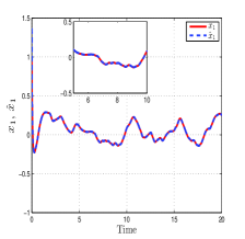
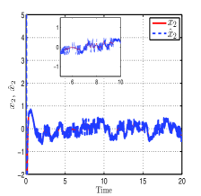
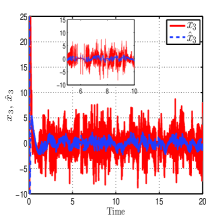
It can be observed from Figure 1 that the estimate effect for both state (x1(t),x2(t))(x_{1}(t),x_{2}(t)) and random total disturbance x3(t)x_{3}(t) and the stabilizing effect for (x1(t),x2(t))(x_{1}(t),x_{2}(t)) are satisfactory, where the estimation effect for x3(t)x_{3}(t) is not as good as the one for state (x1(t),x2(t))(x_{1}(t),x_{2}(t)). These are consistent with the theoretical result presented in Theorem 3.1. 
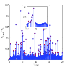
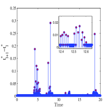
The inter-execution times corresponding to ETM (165) for output transmission and ETM (167) for control signal update can be seen from Figure 2 and Figure 2, respectively, whose respective number of execution times during [0, 20] is 1290 and 8554.

Refer to caption
Refer to caption
Refer to caption
Figure 1: The state and random total disturbance (x1(t),x2(t),x3(t))(x_{1}(t),x_{2}(t),x_{3}(t)) and their estimates (x^1(t),x^2(t),x^3(t))(\hat{x}_{1}(t),\hat{x}_{2}(t),\hat{x}_{3}(t)).
Refer to caption
Refer to caption
Figure 2: Inter-execution times corresponding to ETMs (165) and (167).

6 Concluding remarks

In this paper, event-triggered ADRC has been first addressed for a class of uncertain random nonlinear systems. The controlled systems with lower triangular structure are subject to nonlinear unmodeled dynamics, bounded noise, and colored noise in large scale, whose total effects are treated as a random total disturbance. An event-triggered ESO has been designed for real-time estimation of the random total disturbance, and then an event-triggered controller composed of an output-feedback controller and a compensator has been designed for the output-feedback stabilization and disturbance rejection for the controlled systems. Rigorous theoretical proofs have been given to obtain both the mean square practical convergence and almost surely practical one of the ADRC’s closed-loop under two respective event-triggering mechanisms, validated by some numerical simulations. Potential interesting problems to be solve are the design and convergence analysis of periodic event-triggered ADRC for uncertain random nonlinear systems and the comparison of its communication efficiency with the one of the strategy proposed in this paper.

References

  • [1] Anderson, R. P., Milutinović, D., & Dimarogonas, D. V. (2015). Self-triggered sampling for second-moment stability of state-feedback controlled SDE systems. Automatica, 54, 8-15.
  • [2] Castañeda, L. A., Luviano-Juárez, A., & Chairez, I. (2014). Robust trajectory tracking of a Delta robot through adaptive active disturbance rejection control. IEEE Transactions on Control Systems Technology, 23(4), 1387-1398.
  • [3] Deng, H., & Krstic, M. (1999). Output-feedback stochastic nonlinear stabilization. IEEE Transactions on Automatic Control, 44(2), 328-333.
  • [4] Espitia, N., Karafyllis, I., & Krstic, M. (2021). Event-triggered boundary control of constant-parameter reaction-diffusion PDEs: A small-gain approach. Automatica, 128, 109562.
  • [5] Gauthier, J. P., Hammouri, H., & Othman, S. (1992). A simple observer for nonlinear systems applications to bioreactors. IEEE Transactions on Automatic Control, 37(6), 875-880.
  • [6] Guo, B. Z., Wu, Z. H., & Zhou, H. C. (2015). Active disturbance rejection control approach to output-feedback stabilization of a class of uncertain nonlinear systems subject to stochastic disturbance. IEEE Transactions on Automatic Control, 61(6), 1613-1618.
  • [7] Guo, B. Z., & Zhao, Z. L. (2011). On the convergence of an extended state observer for nonlinear systems with uncertainty. Systems & Control Letters, 60(6), 420-430.
  • [8] Guo, B. Z., & Zhao, Z. L. (2017). Active Disturbance Rejection Control for Nonlinear Systems: An Introduction. John Wiley & Sons, Inc., New York.
  • [9] Han, J. (2009). From PID to active disturbance rejection control. IEEE Transactions on Industrial Electronics, 56(3), 900-906.
  • [10] Heemels, W. H., Donkers, M. C. F., & Teel, A. R. (2012). Periodic event-triggered control for linear systems. IEEE Transactions on Automatic Control, 58(4), 847-861.
  • [11] Huang, Y., Wang, J., Shi, D., Wu, J., & Shi, L. (2019). Event-triggered sampled-data control: An active disturbance rejection approach. IEEE/ASME Transactions on Mechatronics, 24(5), 2052-2063.
  • [12] Huang, Z. L., Zhu, W. Q., Ni, Y. Q., & Ko, J. M. (2002). Stochastic averaging of strongly non-linear oscillators under bounded noise excitation. Journal of Sound and Vibration, 254(2), 245-267.
  • [13] Khas’minskii, R. (1980). Stochastic Stability of Differential Equations. Rockville, MD: S & N International (originally published in Russian by Nauka, Moskow, 1969).
  • [14] Khalil, H. K. (1978). Control of linear singularly perturbed systems with colored noise disturbance. Automatica, 14(2), 153-156.
  • [15] Klosek-Dygas, M. M., Matkowsky, B. J., & Schuss, Z. (1988). Colored noise in dynamical systems. SIAM Journal on Applied Mathematics, 48(2), 425-441.
  • [16] Luo, S., & Deng, F. (2019). On event-triggered control of nonlinear stochastic systems. IEEE Transactions on Automatic Control, 65(1), 369-375.
  • [17] Luo, S., Deng, F., & Chen, W. H. (2019). Dynamic event-triggered control for linear stochastic systems with sporadic measurements and communication delays. Automatica, 107, 86-94.
  • [18] Li, F., & Liu, Y. (2019). Event-triggered stabilization for continuous-time stochastic systems. IEEE Transactions on Automatic Control, 65(10), 4031-4046.
  • [19] Li, F., & Liu, Y. (2020). An enlarged framework of event-triggered control for stochastic systems. IEEE Transactions on Automatic Control, 66(9), 4132-4147.
  • [20] Mao, X. (2007). Stochastic Differential Equations and Applications. Chichester: Horwood Publishing Limited.
  • [21] Ren, H., Cheng, Z., Qin, J., & Lu, R. (2023). Deception attacks on event-triggered distributed consensus estimation for nonlinear systems. Automatica, 154, 111100.
  • [22] Sun, B., & Gao, Z. (2005). A DSP-based active disturbance rejection control design for a 1-kW H-bridge DC-DC power converter. IEEE Transactions on Industrial Electronics, 52(5), 1271-1277.
  • [23] Shi, D., Huang, Y., Wang, J., & Shi, L. (2021). Event-Triggered Active Disturbance Rejection Control. Springer Singapore.
  • [24] Sira-Ramírez, H., Linares-Flores, J., García-Rodríguez, C., & Contreras-Ordaz, M. A. (2014). On the control of the permanent magnet synchronous motor: An active disturbance rejection control approach. IEEE Transactions on Control Systems Technology, 22(5), 2056-2063.
  • [25] Sun, L., Li, D., Hu, K., Lee, K. Y., & Pan, F. (2016). On tuning and practical implementation of active disturbance rejection controller: A case study from a regenerative heater in a 1000 MW power plant. Industrial & Engineering Chemistry Research, 55(23), 6686-6695.
  • [26] Sira-Ramírez, H., Luviano-Juárez, A., Ramírez-Neria, M., & Zurita-Bustamante, E. W. (2017). Active Disturbance Rejection Control of Dynamic Systems: A Flatness Based Approach. Butterworth-Heinemann.
  • [27] Sun, J., Yang, J., Li, S., & Zheng, W. X. (2017). Sampled-data-based event-triggered active disturbance rejection control for disturbed systems in networked environment. IEEE Transactions on Cybernetics, 49(2), 556-566.
  • [28] Texas Instruments, Technical Reference Manual. (2013). TMS320F28069M, TMS320F28068M InstaSPINTM{}^{\mbox{{\small TM}}}-MOTION Software, Literature Number: SPRUHJ0A. April 2013, Revised November 2013.
  • [29] Pan, Z., & Basar, T. (1999). Backstepping controller design for nonlinear stochastic systems under a risk-sensitive cost criterion. SIAM Journal on Control and optimization, 37(3), 957-995.
  • [30] Quevedo, D. E., Gupta, V., Ma, W. J., & Yüksel, S. (2014). Stochastic stability of event-triggered anytime control. IEEE Transactions on Automatic Control, 59(12), 3373-3379.
  • [31] Wu, Z. (2014). Stability criteria of random nonlinear systems and their applications. IEEE Transactions on Automatic Control, 60(4), 1038-1049.
  • [32] Wu, Z. H., Deng, F., Zhou, H. C., & Zhao, Z. L. (2024). Linear and nonlinear event-triggered extended state observers for uncertain random systems. IEEE Transactions on Automatic Control, doi:10.1109/TAC.2024.3370650.
  • [33] Wu, Z., Karimi, H. R., & Shi, P. (2019). Practical trajectory tracking of random Lagrange systems. Automatica, 105, 314-322.
  • [34] Xi, R., Zhang, H., Wang, Y., & Sun, S. (2022). Overview of the recent research progress for stability and control on random nonlinear systems. Annual Reviews in Control, 53, 70-82.
  • [35] Yao, L., Zhang, W., & Xie, X. J. (2020). Stability analysis of random nonlinear systems with time-varying delay and its application. Automatica, 117, 108994.
  • [36] Zhang, H., Xi, R., Wang, Y., Sun, S., & Sun, J. (2021). Event-triggered adaptive tracking control for random systems with coexisting parametric uncertainties and severe nonlinearities. IEEE Transactions on Automatic Control, 67(4), 2011-2018.