This paper was converted on www.awesomepapers.org from LaTeX by an anonymous user.
Want to know more? Visit the Converter page.

Every Bit Counts: Second-Order Analysis of Cooperation in the Multiple-Access Channel

Oliver Kosut, Michelle Effros, Michael Langberg O. Kosut is with the School of Electrical, Computer and Energy Engineering at Arizona State University. Email: okosut@asu.eduM. Effros is with the Department of Electrical Engineering at the California Institute of Technology. Email: effros@caltech.eduM. Langberg is with the Department of Electrical Engineering at the University at Buffalo (State University of New York). Email: mikel@buffalo.eduThis work is supported in part by NSF grants CCF-1817241, CCF-1908725, and CCF-1909451.
Abstract

The work at hand presents a finite-blocklength analysis of the multiple access channel (MAC) sum-rate under the cooperation facilitator (CF) model. The CF model, in which independent encoders coordinate through an intermediary node, is known to show significant rate benefits, even when the rate of cooperation is limited. We continue this line of study for cooperation rates which are sub-linear in the blocklength nn. Roughly speaking, our results show that if the facilitator transmits logK\log{K} bits, there is a sum-rate benefit of order logK/n\sqrt{\log{K}/n}. This result extends across a wide range of KK: even a single bit of cooperation is shown to provide a sum-rate benefit of order 1/n1/\sqrt{n}.

I Introduction

The multiple access channel (MAC) model lies at an interesting conceptual intersection between the notions of cooperation and interference in wireless communications. When viewed from the perspective of any single transmitter, codewords transmitted by other transmitters can only inhibit the first transmitter’s individual communication rate; thus each transmitter sees the others as a source of interference. When viewed from the perspective of the receiver, however, maximizing the total rate delivered to the receiver often requires all transmitters to communicate simultaneously; from the receiver’s perspective, then, the transmitters must cooperate through their simultaneous transmissions to maximize the sum-rate delivered to the receiver.

Simultaneous transmission is, perhaps, the weakest form of cooperation imaginable in a wireless communication model. Nonetheless, the fact that even simultaneous transmission of independent codewords from interfering transmitters can increase the sum-rate deliverable to the MAC receiver begs the question of how much more could be achieved through more significant forms of MAC transmitter cooperation.

The information theory literature devotes considerable effort to studying the impact of encoder cooperation in the MAC. A variety of cooperation models are considered. Examples include the “conferencing” cooperation model [1], in which encoders share information directly in order to coordinate their channel inputs, the “cribbing” cooperation model [2], in which transmitters cooperate by sharing their codeword information (at times causally), and the “cooperation facilitator” (CF) cooperation model [3] in which users coordinate their channel inputs with the help of an intermediary called the CF. The CF distinguishes the amount of information that must be understood to facilitate cooperation (i.e., the rate RINR_{\rm IN} to the CF) from the amount of information employed in the coordination (i.e., the rate ROUTR_{\rm OUT} from the CF). Key results using the CF model show that for many MACs, no matter what the (non-zero) fixed rate CINC_{\rm IN}, the curve describing the maximal sum-rate as a function of ROUTR_{\rm OUT} has infinite slope at ROUT=0R_{\rm OUT}=0 [4]. That is, very little coordination through a CF can change the MAC capacity considerably. This phenomenon holds for both average and maximum error sum-rates; it is most extreme in the latter case, where even a finite number of bits (independent of the blocklength) — that is, ROUT=0R_{\rm OUT}=0 — can suffice to change the MAC capacity region [5, 6, 7].

We study the CF model for 2-user MACs under the average error criterion. In this setting, the maximal sum-rate is a continuous function of ROUTR_{\rm OUT} at ROUT=0R_{\rm OUT}=0 [6, 7], implying a first-order upper-bound on the benefit of cooperation for rates that are sub-linear. However, sub-linear CF cooperation may still increase sum-rate, albeit through second-order terms. In this work, we seek to understand the impact of the CF over a wide range of cooperation rates. Specifically, we consider a CF that, after viewing both messages, can transmit one of KK signals to both transmitters. We prove achievable bounds that express the benefit of this cooperation as a function of KK. These bounds extend all the way from constant KK to exponential KK. Interestingly, we find that even for K=2K=2 (i.e., one bit of cooperation), there is a benefit in the second-order (i.e., dispersion) term, corresponding to an improvement of O(n)O(\sqrt{n}) message bits. We prove two main achievable bounds, each of which is optimal for a different range of KK values. The proof of the first bound is based on refined asymptotic analysis similar to typical second-order bounds. The proof of the second bound is based on the method of types. For a wide range of KK values, we find that the benefit is O(nlogK)O(\sqrt{n\log K}) message bits.

II Problem Setup

An (M1,M2,K)(M_{1},M_{2},K) facilitated multiple access code for multiple access channel (MAC)

(𝒳1×𝒳2,pY|X1,X2(y|x1,x2),𝒴)({\cal X}_{1}\times{\cal X}_{2},p_{Y|X_{1},X_{2}}(y|x_{1},x_{2}),{\cal Y})

is defined by a facilitator code

e:\displaystyle e: [M1]×[M2][K]\displaystyle[M_{1}]\times[M_{2}]\rightarrow[K]

a pair of encoders

f1:\displaystyle f_{1}: [M1]×[K]𝒳1\displaystyle[M_{1}]\times[K]\rightarrow{\cal X}_{1}
f2:\displaystyle f_{2}: [M2]×[K]𝒳2\displaystyle[M_{2}]\times[K]\rightarrow{\cal X}_{2}

and a decoder

g:𝒴[M1]×[M2].g:{\cal Y}\rightarrow[M_{1}]\times[M_{2}].

The encoder’s output is sometimes described using the abbreviated notation

X1(m1,m2)\displaystyle X_{1}(m_{1},m_{2}) =\displaystyle= f1(m1,e(m1,m2))\displaystyle f_{1}(m_{1},e(m_{1},m_{2}))
X2(m1,m2)\displaystyle X_{2}(m_{1},m_{2}) =\displaystyle= f2(m2,e(m1,m2)).\displaystyle f_{2}(m_{2},e(m_{1},m_{2})).

The average error probability for the given code is

Pe\displaystyle P_{e} =1M1M2m1=1M1m2=1M2Pr(g(Y)(m1,m2)|\displaystyle=\frac{1}{M_{1}M_{2}}\sum_{m_{1}=1}^{M_{1}}\sum_{m_{2}=1}^{M_{2}}\Pr\big{(}g(Y)\neq(m_{1},m_{2})\big{|}
(X1,X2)=(X1(m1,m2),X2(m1,m2))).\displaystyle\qquad(X_{1},X_{2})=(X_{1}(m_{1},m_{2}),X_{2}(m_{1},m_{2}))\big{)}.

We also consider codes for the nn-length product channel, where 𝒳1,𝒳2,𝒴{\cal X}_{1},{\cal X}_{2},{\cal Y} are replaced by 𝒳1n,𝒳2n,𝒴n{\cal X}_{1}^{n},{\cal X}_{2}^{n},{\cal Y}^{n} respectively, and where

pYn|X1n,X2n(yn|x1n,x2n)=i=1npY|X1,X2(yi|x1i,x2i).p_{Y^{n}|X_{1}^{n},X_{2}^{n}}(y^{n}|x_{1}^{n},x_{2}^{n})=\prod_{i=1}^{n}p_{Y|X_{1},X_{2}}(y_{i}|x_{1i},x_{2i}).

An (M1,M2,K)(M_{1},M_{2},K) code for the nn-length channel achieving average probability of error at most ϵ\epsilon is called an (n,M1,M2,K,ϵ)(n,M_{1},M_{2},K,\epsilon) code. We assume that all alphabets are finite.

The following notation will be useful. Given a MAC

(𝒳1×𝒳2,pY|X1,X2(y|x1,x2),𝒴),({\cal X}_{1}\times{\cal X}_{2},p_{Y|X_{1},X_{2}}(y|x_{1},x_{2}),{\cal Y}),

the sum-capacity without cooperation is given by

Csum=maxpX1pX2I(X1,X2;Y).C_{\text{sum}}=\max_{p_{X_{1}}p_{X_{2}}}I(X_{1},X_{2};Y). (1)

Let 𝒫{\cal P}^{\star} be the set of product distributions pX1pX2p_{X_{1}}p_{X_{2}} achieving the maximum in (1). For any pX1pX2𝒫p_{X_{1}}p_{X_{2}}\in{\cal P}^{\star}, let pYp_{Y} be the resulting marginal on the channel output, giving

pY(y)=(x1,x2)𝒳1×𝒳2pX1(x1)pX2(x2)pY|X1,X2(y|x1,x2)p_{Y}(y)=\sum_{(x_{1},x_{2})\in{\cal X}_{1}\times{\cal X}_{2}}p_{X_{1}}(x_{1})p_{X_{2}}(x_{2})p_{Y|X_{1},X_{2}}(y|x_{1},x_{2})

for all y𝒴y\in{\cal Y}. We use i(x1,x2;y)i(x_{1},x_{2};y), i(x1;y|x2)i(x_{1};y|x_{2}) and i(x2;y|x1)i(x_{2};y|x_{1}) to represent the joint and conditional information densities

i(x1,x2;y)\displaystyle i(x_{1},x_{2};y) =\displaystyle= log(pY|X1,X2(y|x1,x2)pY(y))\displaystyle\log\left(\frac{p_{Y|X_{1},X_{2}}(y|x_{1},x_{2})}{p_{Y}(y)}\right)
i(x1;y|x2)\displaystyle i(x_{1};y|x_{2}) =\displaystyle= log(pY|X1,X2(y|x1,x2)pY|X2(y|x2))\displaystyle\log\left(\frac{p_{Y|X_{1},X_{2}}(y|x_{1},x_{2})}{p_{Y|X_{2}}(y|x_{2})}\right)
i(x2;y|x1)\displaystyle i(x_{2};y|x_{1}) =\displaystyle= log(pY|X1,X2(y|x1,x2)pY|X1(y|x1)),\displaystyle\log\left(\frac{p_{Y|X_{1},X_{2}}(y|x_{1},x_{2})}{p_{Y|X_{1}}(y|x_{1})}\right),

where pY|X1p_{Y|X_{1}} and pY|X2p_{Y|X_{2}} are conditional marginals on YY under joint distribution

pX1,X2,Y=pX1pX2pY|X1,X2.p_{X_{1},X_{2},Y}=p_{X_{1}}p_{X_{2}}p_{Y|X_{1},X_{2}}.

We denote the 3-vector of all three quantities as

𝐢(x1,x2;y)=[i(x1,x2;y)i(x1;y|x2)i(x2;y|x1)].\mathbf{i}(x_{1},x_{2};y)=\left[\begin{array}[]{c}i(x_{1},x_{2};y)\\ i(x_{1};y|x_{2})\\ i(x_{2};y|x_{1})\end{array}\right].

It will be convenient to define

i(x1,x2)\displaystyle i(x_{1},x_{2}) =E[i(x1,x2;Y)|(X1,X2)=(x1,x2)]\displaystyle=E[i(x_{1},x_{2};Y)|(X_{1},X_{2})=(x_{1},x_{2})]
=D(pY|X1=x1,X2=x2pY).\displaystyle=D(p_{Y|X_{1}=x_{1},X_{2}=x_{2}}\|p_{Y}).

Let

V1\displaystyle V_{1} =Var(i(X1,X2)),\displaystyle=\text{Var}(i(X_{1},X_{2})), (2)
V2\displaystyle V_{2} =E[Var(i(X1,X2;Y)|X1,X2)].\displaystyle=E[\text{Var}(i(X_{1},X_{2};Y)|X_{1},X_{2})]. (3)

Roughly speaking, V1V_{1} represents the information-variance of the codewords, whereas V2V_{2} represents the information-variance of the channel noise. Given two distributions pX,qXp_{X},q_{X}, let the divergence-variance be

V(pXqX)=VarpX(logpX(X)qX(X)).V(p_{X}\|q_{X})=\text{Var}_{p_{X}}\left(\log\frac{p_{X}(X)}{q_{X}(X)}\right).

Note that

V2=x1,x2pX1(x1)pX2(x2)V(pY|X1=x1,X2=x2pY).V_{2}=\sum_{x_{1},x_{2}}p_{X_{1}}(x_{1})p_{X_{2}}(x_{2})V(p_{Y|X_{1}=x_{1},X_{2}=x_{2}}\|p_{Y}).

III Main Results

Define the fundamental sum-rate limit for the facilitated-MAC as

Rsum(n,ϵ,K)=sup{log(M1M2)n:(n,M1,M2,K,ϵ) code}.R_{\text{sum}}(n,\epsilon,K)\\ =\sup\bigg{\{}\frac{\log(M_{1}M_{2})}{n}:\exists(n,M_{1},M_{2},K,\epsilon)\text{ code}\bigg{\}}.

In the literature on second-order rates, there are typically two types of results: (i) finite blocklength results, with no asymptotic terms, that are typically written in terms of abstract alphabets, and (ii) asymptotic results that derive from these finite blocklength results, which are typically easier to understand. The following is an achievable result which has some flavor of both: the channel noise is dealt with via an asymptotic analysis, but the dependence on the randomness in the codewords is written as in a finite blocklength result. We provide this “intermediate” result because, depending on the CF parameter KK, the relevant aspect of the codeword distribution may be in the central limit, moderate deviations, or large deviations regime. Thus, in this form one may plug in any concentration bound to derive an achievable bound. Subsequently, Theorem 2 gives specific achievable results based on two different concentration bounds. We also prove another achievable bound, Theorem 3, which does not rely on Theorem 1, but instead uses an approach based on the method of types that applies at larger values of KK.

Theorem 1.

Assume logK=o(n)\log K=o(n). For any distribution pX1,pX2p_{X_{1}},p_{X_{2}}, let Xjn(k)X_{j}^{n}(k) be an i.i.d. sequence from pXjp_{X_{j}} for each k[K]k\in[K], with all sequences mutually independent. There exists an (n,M1,M2,K,ϵ)(n,M_{1},M_{2},K,\epsilon) code if

ϵ\displaystyle\epsilon Pr(maxk[K]i=1ni(X1i(k),X2i(k))+nV2Z0\displaystyle\geq\Pr\Bigg{(}\max_{k\in[K]}\sum_{i=1}^{n}i(X_{1i}(k),X_{2i}(k))+\sqrt{nV_{2}}\,Z_{0}
<log(M1M2K)+12logn)\displaystyle\qquad<\log(M_{1}M_{2}K)+\frac{1}{2}\log n\Bigg{)}
+O(lognn)+O(logKn)\displaystyle\qquad+O\left(\sqrt{\frac{\log n}{n}}\right)+O\left(\sqrt{\frac{\log K}{n}}\right) (4)
logM1\displaystyle\log M_{1} nI(X1;Y|X2)cnlogK+nlogn\displaystyle\leq nI(X_{1};Y|X_{2})-c\sqrt{n\log K+n\log n} (5)
logM2\displaystyle\log M_{2} nI(X2;Y|X1)cnlogK+nlogn\displaystyle\leq nI(X_{2};Y|X_{1})-c\sqrt{n\log K+n\log n} (6)

where Z0Z_{0} is a standard Gaussian, and where cc is a constant.

For fixed KK, let Z0,,ZKZ_{0},\ldots,Z_{K} be drawn i.i.d. from 𝒩(0,1)\mathcal{N}(0,1). Let

SK=V2Z0+V1maxk[1:K]Zk,S_{K}=\sqrt{V_{2}}\,Z_{0}+\sqrt{V_{1}}\max_{k\in[1:K]}Z_{k},

and define the CDF of SKS_{K} as

FSK(s)=Pr(SKs).F_{S_{K}}(s)=\Pr(S_{K}\leq s).

Also let FSK1F_{S_{K}}^{-1} be the inverse of the CDF; that is,

FSK1(p)=sup{s:FSK(s)p} for p[0,1].F_{S_{K}}^{-1}(p)=\sup\{s:F_{S_{K}}(s)\leq p\}\text{ for }p\in[0,1].

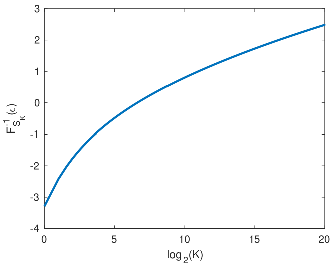
In what follows we use Theorem 1 and the function FSK1F_{S_{K}}^{-1} to explicitly bound from below the benefit in sum-rate when cooperating with varying measures of KK. A numerical computation of FSK1(ϵ)F_{S_{K}}^{-1}(\epsilon) as a function of KK is shown in Fig. 1. The following is a technical estimate of FSK1F_{S_{K}}^{-1}.

Refer to caption
Figure 1: The inverse CDF FSK1(ϵ)F_{S_{K}}^{-1}(\epsilon) for ϵ=0.01\epsilon=0.01, for V1=V2=1V_{1}=V_{2}=1 across a range of KK. Note that the horizontal axis is log2K\log_{2}K, i.e., the number of bits transmitted from the CF.
Lemma 1.

For KK and ϵ\epsilon that satisfy K>e32πln(4/ϵ)K>e^{3}\sqrt{2\pi}\ln(4/\epsilon), FSK1(ϵ)F_{S_{K}}^{-1}(\epsilon) is at least

V1(2lnK2lnln(4/ϵ)lnlnKln(4π))2V2ln(2/ϵ).\sqrt{V_{1}(2\ln K-2\ln\ln({4}/{\epsilon})-\ln\ln K-\ln(4\pi))}\\ -\sqrt{2V_{2}\ln(2/\epsilon)}.

Moreover, for all KK and ϵ\epsilon,

FSK1(1ϵ)2V1lnK+2V1ln(4/ϵ)+2V2ln(2/ϵ).F^{-1}_{S_{K}}(1-\epsilon)\leq\sqrt{2V_{1}\ln K}+\sqrt{2V_{1}\ln(4/\epsilon)}+\sqrt{2V_{2}\ln(2/\epsilon)}.
Proof:

Let Z(K)=maxk[K]ZkZ(K)=\max_{k\in[K]}{Z_{k}}. From [8], it holds that Pr(Z(K)κlnκ)ϵ/2\Pr(Z(K)\leq\sqrt{\kappa-\ln{\kappa}})\leq\epsilon/2 for κ=2ln(K/2π)2lnln(4/ϵ)6\kappa=2\ln(K/\sqrt{2\pi})-2\ln\ln(4/\epsilon)\geq 6. Moreover, Pr(VZ02Vln(2/ϵ))ϵ/2\Pr(\sqrt{V}Z_{0}\leq-\sqrt{2V\ln(2/\epsilon)})\leq\epsilon/2. Combining these bounds gives the desired lower bound.

For the upper bound, [9, 10] imply that for any KK, Pr(V1Z(K)(2V1lnK+2V1ln(4/ϵ)))ϵ/2\Pr(\sqrt{V_{1}}Z(K)\geq(\sqrt{2V_{1}\ln K}+\sqrt{2V_{1}\ln(4/\epsilon)}))\leq\epsilon/2. Moreover, Pr(V2Z02V2ln(2/ϵ))ϵ/2\Pr(\sqrt{V_{2}}Z_{0}\geq\sqrt{2V_{2}\ln(2/\epsilon)})\leq\epsilon/2. Thus, FSk1(1ϵ)2V1lnK+2V1ln(4/ϵ)+2V2ln(2/ϵ)F^{-1}_{S_{k}}(1-\epsilon)\leq\sqrt{2V_{1}\ln K}+\sqrt{2V_{1}\ln(4/\epsilon)}+\sqrt{2V_{2}\ln(2/\epsilon)}. ∎

Theorem 2.

For any pX1pX2𝒫p_{X_{1}}p_{X_{2}}\in{\cal P}^{\star} and the associated constants V1V_{1} and V2V_{2}, if logK=o(n1/3)\log K=o(n^{1/3}), then

Rsum(n,ϵ,K)Csum+1nFSK1(ϵ)θnR_{\text{sum}}(n,\epsilon,K)\geq C_{\text{sum}}+\frac{1}{\sqrt{n}}\,F_{S_{K}}^{-1}(\epsilon)-\theta_{n}

where

θn\displaystyle\theta_{n} =O(lognn),\displaystyle=O\left(\frac{\log n}{n}\right), if Klogn\displaystyle\text{ if }K\leq\log n (7)
θn\displaystyle\theta_{n} =O(Kn),\displaystyle=O\left(\frac{K}{n}\right), if lognKlog3/2n\displaystyle\text{ if }\log n\leq K\leq\log^{3/2}n (8)
θn\displaystyle\theta_{n} =O(log3/2nn),\displaystyle=O\left(\frac{\log^{3/2}n}{n}\right), if log3/2nKn\displaystyle\text{ if }\log^{3/2}n\leq K\leq n (9)
θn\displaystyle\theta_{n} =O(log3/2Kn),\displaystyle=O\left(\frac{\log^{3/2}K}{n}\right), if Kn.\displaystyle\text{ if }K\geq n. (10)

For larger KK, our achievability bound employs the function

Δ(a)=maxpX1,X2:I(X1;X2)aI(X1,X2;Y)Csum.\Delta(a)=\max_{p_{X_{1},X_{2}}:I(X_{1};X_{2})\leq a}I(X_{1},X_{2};Y)-C_{\text{sum}}.

Note that Δ(0)=0\Delta(0)=0. Lemma 2 captures the behavior of Δ(a)\Delta(a) for small aa. (See Appendix A for the proof.)

Lemma 2.

In the limit as a0a\to 0,

Δ(a)=a 2V1ln2+o(a)\Delta(a)=\sqrt{a\,2V_{1}^{\star}\ln 2}+o(\sqrt{a})

where

V1=maxpX1pX2𝒫Var(i(X1,X2)).V_{1}^{\star}=\max_{p_{X_{1}}p_{X_{2}}\in{\cal P}^{\star}}\text{{\em Var}}(i(X_{1},X_{2})). (11)
Theorem 3.

For any KK such that logK=ω(logn)\log K=\omega(\log n),

Rsum(n,ϵ,K)Csum+Δ(logKnO(lognn))O(1n).R_{\text{sum}}(n,\epsilon,K)\\ \geq C_{\text{sum}}+\Delta\left(\frac{\log K}{n}-O\left(\frac{\log n}{n}\right)\right)-O\left(\frac{1}{\sqrt{n}}\right).
Remark 1.

While Theorems 2 and 3 appear quite different, Lemmas 1 and 2 imply that for mid-range KK values, they give similar results. In particular, if

lognlogKn1/3\log n\ll\log K\ll n^{1/3}

then applying Theorem 2, and choosing the distribution pX1pX2𝒫p_{X_{1}}p_{X_{2}}\in{\cal P}^{\star} that achieves the maximum in (11) gives

Rsum(n,ϵ,K)Csum\displaystyle R_{\text{sum}}(n,\epsilon,K)-C_{\text{sum}} 1nFSK1(ϵ)θn\displaystyle\geq\frac{1}{\sqrt{n}}F_{S_{K}}^{-1}(\epsilon)-\theta_{n}
2V1lnKn.\displaystyle\approx\sqrt{\frac{2V_{1}^{\star}\ln K}{n}}.

For the same range of KK, Theorem 3 gives

Rsum(n,ϵ,K)Csum\displaystyle R_{\text{sum}}(n,\epsilon,K)-C_{\text{sum}} Δ(logKnO(lognn))\displaystyle\geq\Delta\left(\frac{\log K}{n}-O\left(\frac{\log n}{n}\right)\right)
O(1n)\displaystyle\qquad-O\left(\frac{1}{\sqrt{n}}\right)
V1logKn 2ln2\displaystyle\approx\sqrt{\frac{V_{1}^{\star}\log K}{n}\,2\ln 2}
=2V1lnKn.\displaystyle=\sqrt{\frac{2V_{1}^{\star}\ln K}{n}}.

III-A Comparison to prior work

In [4], an analog to Theorem 3 is proven for the asymptotic blocklength regime. Namely, in our notation, [4] proves that for any ϵ>0\epsilon>0 and δ>0\delta>0, if we set K=2Ω(n)K=2^{\Omega(n)} then there exist nn such that,

Rsum(n,ϵ,K)Csum>Δ(logKn)δ.R_{\text{sum}}(n,\epsilon,K)-C_{\text{sum}}>\Delta\left(\frac{\log{K}}{n}\right)-\delta.

Similarly, in [4, 7], an analog to Lemma 2 is shown for asymptotic blocklength. Specifically, it is shown that the existence of distributions pX1pX2𝒫p_{X_{1}}p_{X_{2}}\in{\cal P}^{\star} and pX~1X~2p_{\tilde{X}_{1}\tilde{X}_{2}} over 𝒳1×𝒳2{\cal X}_{1}\times{\cal X}_{2} such that (a) the support of pX~1X~2p_{\tilde{X}_{1}\tilde{X}_{2}} is included in that of pX1pX2p_{X_{1}}p_{X_{2}}, and (b)

I(X~1,X~2,Y~)+D(pX~1X~2pX1pX2)>I(X1,X2;Y)I(\tilde{X}_{1},\tilde{X}_{2},\tilde{Y})+D(p_{\tilde{X}_{1}\tilde{X}_{2}}\|p_{X_{1}}p_{X_{2}})>I(X_{1},X_{2};Y)

for

pX1,X2,X~1,X~2,Y,Y~(x1,x2,x~1,x~2,y,y~)\displaystyle p_{X_{1},X_{2},\tilde{X}_{1},\tilde{X}_{2},Y,\tilde{Y}}(x_{1},x_{2},\tilde{x}_{1},\tilde{x}_{2},y,\tilde{y})
=pX1(x1)pX2(x2)pX~1,X~2(x~1,x~2)\displaystyle=p_{X_{1}}(x_{1})p_{X_{2}}(x_{2})p_{\tilde{X}_{1},\tilde{X}_{2}}(\tilde{x}_{1},\tilde{x}_{2})
pY|X1,X2(y|x1,x2)pY|X1,X2(y~|x~1,x~2),\displaystyle\qquad\cdot p_{Y|X_{1},X_{2}}(y|x_{1},x_{2})p_{Y|X_{1},X_{2}}(\tilde{y}|\tilde{x}_{1},\tilde{x}_{2}),

imply that there exists a constant σ0\sigma_{0} such that

lima0Δ(a)σ0a.\lim_{a\rightarrow 0}\Delta(a)\geq\sigma_{0}\sqrt{a}.

Although Theorem 3 and Lemma 2 (and their proof techniques) are similar in nature to those of [4, 7], the analysis presented here is refined in that it captures higher order behavior in blocklength nn and further optimized to address the challenges in studying values of KK that are sub-exponential in the blocklength nn.

We may also compare our results against prior achievable bounds without cooperation. Note that the standard MAC, with no cooperation, corresponds to K=1K=1. In fact, in this case Theorem 2 gives the same second-order term as the best-known achievable bound for the MAC sum-rate [11, 12, 13, 14, 15]. This can be seen by noting that S1𝒩(0,V1+V2)S_{1}\sim\mathcal{N}(0,V_{1}+V_{2}), and so FS11(ϵ)=V1+V2Φ1(ϵ)F_{S_{1}}^{-1}(\epsilon)=\sqrt{V_{1}+V_{2}}\Phi^{-1}(\epsilon). Thus Theorem 2 gives

Rsum(n,ϵ,1)Csum+V1+V2nΦ1(ϵ)O(lognn).R_{\text{sum}}(n,\epsilon,1)\geq C_{\text{sum}}+\sqrt{\frac{V_{1}+V_{2}}{n}}\Phi^{-1}(\epsilon)-O\left(\frac{\log n}{n}\right).

Moreover,

V1+V2=Var(i(X1,X2;Y))V_{1}+V_{2}=\text{Var}(i(X_{1},X_{2};Y))

which, for the optimal input distribution, is precisely the best-known achievable dispersion. The proof of Theorem 2 uses i.i.d. codebooks, which, as shown in [14], can be outperformed in terms of second-order rate by constant combination codebooks. However, as pointed out in [15, Sec. III-B], the two approaches give the same bounds on the sum-rate itself.

Another interesting conclusion comes from comparing the no cooperation case (K=1K=1) with a single bit of cooperation (K=2K=2). As long as V1>0V_{1}^{\star}>0, it is easy to see that FS21(ϵ)>FS11(ϵ)F_{S_{2}}^{-1}(\epsilon)>F_{S_{1}}^{-1}(\epsilon) for any ϵ(0,1)\epsilon\in(0,1) (Fig. 1 shows an example). Thus, the second-order coefficient in Theorem 2 for K=2K=2 is strictly improved compared to K=1K=1. Therefore, even a single bit of cooperation allows for O(n)O(\sqrt{n}) additional message bits.

IV Proof of Theorem 1

We use random code design, beginning with independent design of the codewords for both transmitters. Precisely, we draw

f1(1,1),f1(1,2),,f1(M1,K)\displaystyle f_{1}(1,1),f_{1}(1,2),\ldots,f_{1}(M_{1},K) \displaystyle\sim i.i.d. pX1\displaystyle\mbox{i.i.d. }p_{X_{1}}
f2(1,1),f2(1,2),,f2(M2,K)\displaystyle f_{2}(1,1),f_{2}(1,2),\ldots,f_{2}(M_{2},K) \displaystyle\sim i.i.d. pX2.\displaystyle\mbox{i.i.d. }p_{X_{2}}.

The facilitator code e(m1,m2)e(m_{1},m_{2}) is then designed in an attempt to maximize the likelihood pY|X1,X2p_{Y|X_{1},X_{2}} under a received channel output YY. We begin by defining the threshold decoder g(y)g(y) employed in our analysis. Maximum likelihood decoding is expected to give the best performance, but instead we here employ a threshold decoder for simplicity. For notational efficiency, let

(X1,X2)(m1,m2)=(X1(m1,m2),X2(m1,m2))\displaystyle(X_{1},X_{2})(m_{1},m_{2})=(X_{1}(m_{1},m_{2}),X_{2}(m_{1},m_{2}))
=(f1(m1,e(m1,m2)),f2(m2,e(m1,m2))),\displaystyle=(f_{1}(m_{1},e(m_{1},m_{2})),f_{2}(m_{2},e(m_{1},m_{2}))),

where e(m1,m2)e(m_{1},m_{2}) is the (fixed) facilitator function to be defined below. Given a constant vector 𝐜=[c12,c1,c2]T\mathbf{c}^{\star}=[c_{12}^{\star},c_{1}^{\star},c_{2}^{\star}]^{T}, we define the decoder g(y)g(y) to choose the unique message pair (m1,m2)(m_{1},m_{2}) such that

𝐢((X1,X2)(m1,m2);y)𝐜,\mathbf{i}((X_{1},X_{2})(m_{1},m_{2});y)\geq\mathbf{c}^{\star},

where the vector inequality means that all three inequalities must hold simultaneously. Conversely we use the notation \not\geq between vectors to mean that any one of the three inequalities fails. If the number of message pairs that meet this constraint is not one, we declare an error. In an attempt to ensure that i((X1,X2)(m1,m2);Y)i((X_{1},X_{2})(m_{1},m_{2});Y) is, in some sense, large for random channel outputs YY that may result from that codeword pair’s transmissions, for each (m1,m2)[M1]×[M2](m_{1},m_{2})\in[M_{1}]\times[M_{2}], we define

e(m1,m2)=argmaxk[K]s(f1(m1,k),f2(m2,k)),e(m_{1},m_{2})=\operatorname*{arg\,max}_{k\in[K]}s(f_{1}(m_{1},k),f_{2}(m_{2},k)),

where s(x1,x2)s(x_{1},x_{2}) is a score function to be chosen below.

Under this code design, the expected error probability satisfies

E[Pe]=E[Pr(g(Y)(1,1)|(X1,X2)=(X1,X2)(1,1))]Pr(𝐢((X1,X2)(m1,m2);Y)𝐜 or 𝐢(X1(m^1,k^),X2(m^2,k^);Y)𝐜 for any (m^1,m^2)(1,1),k[K]|(X1,X2)=(X1,X2)(1,1)).\begin{array}[]{r@{}l}\lx@intercol\hfil E[P_{e}]=E\left[\Pr\left(\left.g(Y)\neq(1,1)\right|(X_{1},X_{2})=(X_{1},X_{2})(1,1)\right)\right]\hfil\lx@intercol\\ \leq\Pr\Bigg{(}&\mathbf{i}((X_{1},X_{2})(m_{1},m_{2});Y)\not\geq\mathbf{c}^{\star}\\ &\text{ or }\mathbf{i}(X_{1}(\hat{m}_{1},\hat{k}),X_{2}(\hat{m}_{2},\hat{k});Y)\geq\mathbf{c}^{\star}\\ &\text{ for any }(\hat{m}_{1},\hat{m}_{2})\neq(1,1),k\in[K]\\ &\Bigg{|}(X_{1},X_{2})=(X_{1},X_{2})(1,1)\Bigg{)}.\end{array}

To further upper bound the error probability, we define the following random variables. Let pX~1,X~2p_{\tilde{X}_{1},\tilde{X}_{2}} be the joint distribution of (X1,X2)(1,1)(X_{1},X_{2})(1,1) that results from our choice of CF. This distribution would be the same for any message pair. Let variables X1X_{1}, X2X_{2}, X~1\tilde{X}_{1}, X~2\tilde{X}_{2}, YY, Y~\tilde{Y} have joint distribution

pX1,X2,X~1,X~2,Y,Y~(x1,x2,x~1,x~2,y,y~)\displaystyle p_{X_{1},X_{2},\tilde{X}_{1},\tilde{X}_{2},Y,\tilde{Y}}(x_{1},x_{2},\tilde{x}_{1},\tilde{x}_{2},y,\tilde{y})
=pX1(x1)pX2(x2)pX~1,X~2(x~1,x~2)\displaystyle=p_{X_{1}}(x_{1})p_{X_{2}}(x_{2})p_{\tilde{X}_{1},\tilde{X}_{2}}(\tilde{x}_{1},\tilde{x}_{2})
pY|X1,X2(y|x1,x2)pY|X1,X2(y~|x~1,x~2).\displaystyle\qquad\cdot p_{Y|X_{1},X_{2}}(y|x_{1},x_{2})p_{Y|X_{1},X_{2}}(\tilde{y}|\tilde{x}_{1},\tilde{x}_{2}).

Under transmission of message pair (1,1)(1,1), (X1,X2,Y)(X_{1},X_{2},Y) capture the relationship between channel inputs and output in a standard MAC, whereas (X~1,X~2,Y~)(\tilde{X}_{1},\tilde{X}_{2},\tilde{Y}) capture the corresponding relationship with CF. Moreover, (X~1,X2,Y~)(\tilde{X}_{1},X_{2},\tilde{Y}), (X1,X~2,Y~)(X_{1},\tilde{X}_{2},\tilde{Y}), and (X1,X2,Y~)(X_{1},X_{2},\tilde{Y}) capture the relationship between the channel output and one or more untransmitted codewords from our random code. Assume without loss of generality that e(1,1)=1e(1,1)=1; i.e., (X1,X2)(1,1)=(f1(1,1),f2(1,1))(X_{1},X_{2})(1,1)=(f_{1}(1,1),f_{2}(1,1)). We now analyze the error probability by considering the following cases.

m^1\hat{m}_{1} m^2\hat{m}_{2} k^\hat{k} Number of values Distribution
1\neq 1 1 1 M11M_{1}-1 pX1pX~2,Y~p_{X_{1}}p_{\tilde{X}_{2},\tilde{Y}}
1\neq 1 1 1\neq 1 (M11)(K1)(M_{1}-1)(K-1) pX1pX2pY~p_{X_{1}}p_{X_{2}}p_{\tilde{Y}}
1 1\neq 1 1 M21M_{2}-1 pX~1,Y~pX2p_{\tilde{X}_{1},\tilde{Y}}p_{X_{2}}
11 1\neq 1 1\neq 1 (M21)(K1)(M_{2}-1)(K-1) pX1pX2pY~p_{X_{1}}p_{X_{2}}p_{\tilde{Y}}
1\neq 1 1\neq 1 any (M11)(M21)K(M_{1}-1)(M_{2}-1)K pX1pX2pY~p_{X_{1}}p_{X_{2}}p_{\tilde{Y}}

Note that we have excluded cases where m^1=m^2=1\hat{m}_{1}=\hat{m}_{2}=1, since those are not errors (even if k^1\hat{k}\neq 1). Moreover, the number of cases wherein X1(m^1,k^),X2(m^2,k^),YX_{1}(\hat{m}_{1},\hat{k}),X_{2}(\hat{m}_{2},\hat{k}),Y has joint distribution pX1pX2pY~p_{X_{1}}p_{X_{2}}p_{\tilde{Y}} is less than M1M2KM_{1}M_{2}K. We can upper bound the expected error probability as

E[Pe]\displaystyle E[P_{e}] Pr(𝐢(X~1,X~2;Y~)𝐜)\displaystyle\leq\Pr\left(\mathbf{i}(\tilde{X}_{1},\tilde{X}_{2};\tilde{Y})\not\geq\mathbf{c}^{\star}\right)
+M1M2KPr(𝐢(X1,X2;Y~)𝐜)\displaystyle\quad+M_{1}M_{2}K\Pr(\mathbf{i}(X_{1},X_{2};\tilde{Y})\geq\mathbf{c}^{\star})
+M1Pr(𝐢(X1,X~2;Y~)𝐜)\displaystyle\quad+M_{1}\Pr(\mathbf{i}(X_{1},\tilde{X}_{2};\tilde{Y})\geq\mathbf{c}^{\star})
+M2Pr(𝐢(X~1,X2;Y~)𝐜))\displaystyle\quad+M_{2}\Pr(\mathbf{i}(\tilde{X}_{1},X_{2};\tilde{Y})\geq\mathbf{c}^{\star}))
Pr(𝐢(X~1,X~2;Y~)𝐜)\displaystyle\leq\Pr\left(\mathbf{i}(\tilde{X}_{1},\tilde{X}_{2};\tilde{Y})\not\geq\mathbf{c}^{\star}\right)
+M1M2KPr(i(X1,X2;Y~)c12)\displaystyle\quad+M_{1}M_{2}K\Pr(i(X_{1},X_{2};\tilde{Y})\geq c_{12}^{\star})
+M1Pr(i(X1;Y~|X~2)c1)\displaystyle\quad+M_{1}\Pr(i(X_{1};\tilde{Y}|\tilde{X}_{2})\geq c_{1}^{\star})
+M2Pr(i(X2;Y~|X~1)c2)\displaystyle\quad+M_{2}\Pr(i(X_{2};\tilde{Y}|\tilde{X}_{1})\geq c_{2}^{\star})

Note that

Pr(i(X1;Y~|X~2)c1)\displaystyle\Pr(i(X_{1};\tilde{Y}|\tilde{X}_{2})\geq c_{1}^{\star})
=x1,x2,ypX1(x1)pX~2,Y~(x2,y)1(i(x1;y|x2)c1)\displaystyle=\sum_{x_{1},x_{2},y}p_{X_{1}}(x_{1})p_{\tilde{X}_{2},\tilde{Y}}(x_{2},y)1\left(i(x_{1};y|x_{2})\geq c_{1}^{\star}\right)
=x1,x2,ypX1|X2(x1|x2)pX~2,Y~(x2,y)\displaystyle=\sum_{x_{1},x_{2},y}p_{X_{1}|X_{2}}(x_{1}|x_{2})p_{\tilde{X}_{2},\tilde{Y}}(x_{2},y)
1(i(x1;y|x2)c1)\displaystyle\quad\cdot 1\left(i(x_{1};y|x_{2})\geq c_{1}^{\star}\right)
=x2,ypX~2,Y~(x2,y)x1pX1|X2,Y(x1|x2,y)\displaystyle=\sum_{x_{2},y}p_{\tilde{X}_{2},\tilde{Y}}(x_{2},y)\sum_{x_{1}}p_{X_{1}|X_{2},Y}(x_{1}|x_{2},y)
pX1|X2(x1|x2)pX1|X2,Y(x1|x2,y)1(i(x1;y|x2)c1)\displaystyle\quad\cdot\frac{p_{X_{1}|X_{2}}(x_{1}|x_{2})}{p_{X_{1}|X_{2},Y}(x_{1}|x_{2},y)}1\left(i(x_{1};y|x_{2})\geq c_{1}^{\star}\right)
=x2,ypX~2,Y~(x2,y)x1pX1|X2,Y(x1|x2,y)\displaystyle=\sum_{x_{2},y}p_{\tilde{X}_{2},\tilde{Y}}(x_{2},y)\sum_{x_{1}}p_{X_{1}|X_{2},Y}(x_{1}|x_{2},y)
pY|X2(y|x2)pY|X1,X2(y|x1,x2)\displaystyle\quad\cdot\frac{p_{Y|X_{2}}(y|x_{2})}{p_{Y|X_{1},X_{2}}(y|x_{1},x_{2})}
1(logpY|X1,X2(y|x1,x2)pY|X2(y|x2)c1)\displaystyle\quad\cdot 1\left(\log\frac{p_{Y|X_{1},X_{2}}(y|x_{1},x_{2})}{p_{Y|X_{2}}(y|x_{2})}\geq c_{1}^{\star}\right)
x2,ypX~2,Y~(x2,y)x1pX1|X2,Y(x1|x2,y)exp(c1)\displaystyle\leq\sum_{x_{2},y}p_{\tilde{X}_{2},\tilde{Y}}(x_{2},y)\sum_{x_{1}}p_{X_{1}|X_{2},Y}(x_{1}|x_{2},y)\exp(-c_{1}^{\star})
=exp(c1).\displaystyle=\exp(-c_{1}^{\star}).

Applying similar arguments to the other terms, we find

E[Pe]\displaystyle E[P_{e}] Pr(𝐢(X~1,X~2;Y~)𝐜)+M1M2Kexp(c12)\displaystyle\leq\Pr\left(\mathbf{i}(\tilde{X}_{1},\tilde{X}_{2};\tilde{Y})\not\geq\mathbf{c}^{\star}\right)+M_{1}M_{2}K\exp(-c_{12}^{\star})
+M1exp(c1)+M2exp(c2).\displaystyle\quad+M_{1}\exp(-c_{1}^{\star})+M_{2}\exp(-c_{2}^{\star}). (12)

Note that (12) may be viewed as a finite blocklength achievable result. While our primary goal is asymptotic second-order analysis, we proceed by analyzing this bound on the nn-length product channel. Specifically, we now focus on the case where (𝒳1×𝒳2,pY|X1,X2,𝒴)({\cal X}_{1}\times{\cal X}_{2},p_{Y|X_{1},X_{2}},{\cal Y}) captures nn uses of a discrete, memoryless channel. We designate this special case by

(𝒳1n×𝒳2n,(pY|X1,X2)n,𝒴n)({\cal X}_{1}^{n}\times{\cal X}_{2}^{n},(p_{Y|X_{1},X_{2}})^{n},{\cal Y}^{n})

and add superscript nn to all coding functions as a reminder of the scenario in operation. Assume that each codeword entry is drawn i.i.d. from pX1p_{X_{1}} or pX2p_{X_{2}}. Define the CF’s score function as

s(x1n,x2n)=i=1ni(x1i,x2i).s(x_{1}^{n},x_{2}^{n})=\sum_{i=1}^{n}i(x_{1i},x_{2i}).

If we choose

c12\displaystyle c_{12}^{\star} =log(M1M2K)+12logn,\displaystyle=\log(M_{1}M_{2}K)+\frac{1}{2}\log n,
c1\displaystyle c_{1}^{\star} =logM1+12logn,\displaystyle=\log M_{1}+\frac{1}{2}\log n,
c2\displaystyle c_{2}^{\star} =logM2+12logn,\displaystyle=\log M_{2}+\frac{1}{2}\log n,

then

E[Pe]Pr(𝐢(X~1n,X~2n;Y~n)𝐜)+3n\displaystyle E[P_{e}]\leq\Pr\left(\mathbf{i}(\tilde{X}_{1}^{n},\tilde{X}_{2}^{n};\tilde{Y}^{n})\not\geq\mathbf{c}^{\star}\right)+\frac{3}{\sqrt{n}}
Pr(i(X~1n,X~2n;Y~n)<log(M1M2K)+12logn)\displaystyle\leq\Pr\left(i(\tilde{X}_{1}^{n},\tilde{X}_{2}^{n};\tilde{Y}^{n})<\log(M_{1}M_{2}K)+\frac{1}{2}\log n\right)
+Pr(i(X~1n;Y~n|X~2n)<logM1+12logn)\displaystyle\quad+\Pr\left(i(\tilde{X}_{1}^{n};\tilde{Y}^{n}|\tilde{X}_{2}^{n})<\log M_{1}+\frac{1}{2}\log n\right)
+Pr(i(X~2n;Y~n|X~1n)<logM2+12logn)+3n.\displaystyle\quad+\Pr\left(i(\tilde{X}_{2}^{n};\tilde{Y}^{n}|\tilde{X}_{1}^{n})<\log M_{2}+\frac{1}{2}\log n\right)+\frac{3}{\sqrt{n}}. (13)

We begin by bounding the second and third terms of (13) before returning to bound the first. For the second term in (13), recall that X~1n,X~2n\tilde{X}_{1}^{n},\tilde{X}_{2}^{n} are drawn from the distribution of (X1n,X2n)(1,1)(X_{1}^{n},X_{2}^{n})(1,1) induced by the cooperation facilitator,

Pr(i(X~1n;Y~n|X~2n)<logM1+12logn)\displaystyle\Pr\left(i(\tilde{X}_{1}^{n};\tilde{Y}^{n}|\tilde{X}_{2}^{n})<\log M_{1}+\frac{1}{2}\log n\right) (14)
KPr(i(X1n;Yn|X2n)<logM1+12logn)\displaystyle\leq K\Pr\left(i(X_{1}^{n};Y^{n}|X_{2}^{n})<\log M_{1}+\frac{1}{2}\log n\right)
Kexp{a1n(nI(X1;Y|X2)logM112logn)2}\displaystyle\leq K\exp\left\{-\frac{a_{1}}{n}\left(nI(X_{1};Y|X_{2})-\log M_{1}-\frac{1}{2}\log n\right)^{2}\right\}

where the last inequality follows from Hoeffding’s inequality and the assumption that i(X1;Y|X2)i(X_{1};Y|X_{2}) is bounded, where a1a_{1} is a constant employed in this bound. By the assumption of logM1\log M_{1} in the statement of the theorem, this quantity is at most 1/n1/\sqrt{n} for a suitable constant cc. A similar bound can be applied to the third term in (13).

Now we consider the first term in (13). For fixed x1n,x2nx_{1}^{n},x_{2}^{n},

E[i(x1n,x2n;Yn)]=i=1ni(x1i,x2i)=s(x1n,x2n).E[i(x_{1}^{n},x_{2}^{n};Y^{n})]=\sum_{i=1}^{n}i(x_{1i},x_{2i})=s(x_{1}^{n},x_{2}^{n}).

Thus we can apply the Berry-Esseen theorem to write

Pr(i(x1n,x2n;Yn)<c12|(X1n,X2n)=(x1n,x2n))\displaystyle\Pr\bigg{(}i(x_{1}^{n},x_{2}^{n};Y^{n})<c_{12}^{\star}\bigg{|}(X_{1}^{n},X_{2}^{n})=(x_{1}^{n},x_{2}^{n})\bigg{)}
Pr(s(x1n,x2n)+i=1nV(p(y|x1i,x2i)pY)Z0\displaystyle\leq\Pr\bigg{(}s(x_{1}^{n},x_{2}^{n})+\sqrt{\sum_{i=1}^{n}V(p(y|x_{1i},x_{2i})\|p_{Y})}\,Z_{0}
<c12)+Bn\displaystyle\qquad<c_{12}^{\star}\bigg{)}+\frac{B}{\sqrt{n}}

where, as in the statement of the theorem, Z0Z_{0} is a standard Gaussian random variable.

Assume

V(pY|X1=x1,X2=x2pY)Vmax for all x1,x2.V(p_{Y|X_{1}=x_{1},X_{2}=x_{2}}\|p_{Y})\leq V_{\max}\text{ for all }x_{1},x_{2}.

Let

γ=VmaxlnK+12lnn2n.\gamma=V_{\max}\sqrt{\frac{\ln K+\frac{1}{2}\ln n}{2n}}.

Note that

γ=O(logKn)+O(lognn).\gamma=O\left(\sqrt{\frac{\log K}{n}}\right)+O\left(\sqrt{\frac{\log n}{n}}\right).

By the assumption that logK=o(n)\log K=o(n), γ=o(1)\gamma=o(1). By Hoeffding’s inequality, we may write

Pr(|1ni=1nV(p(y|X1i,X2i)pY)V2|>γ)\displaystyle\Pr\left(\left|\frac{1}{n}\sum_{i=1}^{n}V(p(y|X_{1i},X_{2i})\|p_{Y})-V_{2}\right|>\gamma\right)
2exp{2nγ2Vmax2}=2Kn.\displaystyle\leq 2\exp\left\{-\frac{2n\gamma^{2}}{V_{\max}^{2}}\right\}=\frac{2}{K\sqrt{n}}.

Thus, by the union bound

Pr(|1ni=1nV(p(y|f1i(1,k),f2i(1,k))pY)V2|>γ for any k[K])2n.\Pr\Bigg{(}\Bigg{|}\frac{1}{n}\sum_{i=1}^{n}V(p(y|f_{1i}(1,k),f_{2i}(1,k))\|p_{Y})-V_{2}\Bigg{|}>\gamma\\ \text{ for any }k\in[K]\Bigg{)}\leq\frac{2}{\sqrt{n}}.

Thus

E[Pe]Pr(s(X~1n,X~2n)\displaystyle E[P_{e}]\leq\Pr\Bigg{(}s(\tilde{X}_{1}^{n},\tilde{X}_{2}^{n})
+i=1nV(p(y|X~1i,X~2i)pY)Z0<c12)+O(1n)\displaystyle\quad+\sqrt{\sum_{i=1}^{n}V(p(y|\tilde{X}_{1i},\tilde{X}_{2i})\|p_{Y})}\,Z_{0}<c_{12}^{\star}\Bigg{)}+O\left(\frac{1}{\sqrt{n}}\right)
E[maxV[V2γ,V2+γ]Pr(s(X~1n,X~2n)+nVZ0\displaystyle\leq E\Bigg{[}\max_{V^{\prime}\in[V_{2}-\gamma,V_{2}+\gamma]}\Pr\Bigg{(}s(\tilde{X}_{1}^{n},\tilde{X}_{2}^{n})+\sqrt{nV^{\prime}}\,Z_{0}
<c12|X~1n,X~2n)]+O(1n)\displaystyle\qquad<c_{12}^{\star}\Bigg{|}\tilde{X}_{1}^{n},\tilde{X}_{2}^{n}\Bigg{)}\Bigg{]}+O\left(\frac{1}{\sqrt{n}}\right)
=E[maxV[V2γ,V2+γ]Φ(c12s(X~1n,X~2n)nV)]\displaystyle=E\Bigg{[}\max_{V^{\prime}\in[V_{2}-\gamma,V_{2}+\gamma]}\Phi\left(\frac{c_{12}^{\star}-s(\tilde{X}_{1}^{n},\tilde{X}_{2}^{n})}{\sqrt{nV^{\prime}}}\right)\Bigg{]}
+O(1n)\displaystyle\quad+O\left(\frac{1}{\sqrt{n}}\right)

where Φ()\Phi(\cdot) is the Gaussian CDF. Similarly, let ϕ()\phi(\cdot) be the Gaussian PDF. Given x1n,x2nx_{1}^{n},x_{2}^{n}, let

z=c12s(x1n,x2n)n.z=\frac{c_{12}^{\star}-s(x_{1}^{n},x_{2}^{n})}{\sqrt{n}}.

If z0z\geq 0, then we may bound

maxV[V2γ,V2+γ]Φ(zV)\displaystyle\max_{V^{\prime}\in[V_{2}-\gamma,V_{2}+\gamma]}\Phi\left(\frac{z}{\sqrt{V^{\prime}}}\right)
=Φ(zV2γ)\displaystyle=\Phi\left(\frac{z}{\sqrt{V_{2}-\gamma}}\right)
=Φ(zV2)+z/V2z/V2γϕ(y)𝑑y\displaystyle=\Phi\left(\frac{z}{\sqrt{V_{2}}}\right)+\int_{z/\sqrt{V_{2}}}^{z/\sqrt{V_{2}-\gamma}}\phi(y)dy
Φ(zV2)+(1V2γ1V2)zϕ(zV2)\displaystyle\leq\Phi\left(\frac{z}{\sqrt{V_{2}}}\right)+\left(\frac{1}{\sqrt{V_{2}-\gamma}}-\frac{1}{\sqrt{V_{2}}}\right)z\phi\left(\frac{z}{\sqrt{V_{2}}}\right)
Φ(zV2)+(1V2γ1V2)V22πe\displaystyle\leq\Phi\left(\frac{z}{\sqrt{V_{2}}}\right)+\left(\frac{1}{\sqrt{V_{2}-\gamma}}-\frac{1}{\sqrt{V_{2}}}\right)\sqrt{\frac{V_{2}}{2\pi e}}
=Φ(zV2)+(V2V2γ1)12πe.\displaystyle=\Phi\left(\frac{z}{\sqrt{V_{2}}}\right)+\left(\sqrt{\frac{V_{2}}{V_{2}-\gamma}}-1\right)\frac{1}{\sqrt{2\pi e}}.

If z0z\geq 0, then we may bound

maxV[V2γ,V2+γ]Φ(zV)\displaystyle\max_{V^{\prime}\in[V_{2}-\gamma,V_{2}+\gamma]}\Phi\left(\frac{z}{\sqrt{V^{\prime}}}\right)
=Φ(zV2+γ)\displaystyle=\Phi\left(\frac{z}{\sqrt{V_{2}+\gamma}}\right)
=Φ(zV2)+z/V2z/V2+γϕ(y)𝑑y\displaystyle=\Phi\left(\frac{z}{\sqrt{V_{2}}}\right)+\int_{z/\sqrt{V_{2}}}^{z/\sqrt{V_{2}+\gamma}}\phi(y)dy
Φ(zV2)+(1V21V2+γ)|z|ϕ(zV2+γ)\displaystyle\leq\Phi\left(\frac{z}{\sqrt{V_{2}}}\right)+\left(\frac{1}{\sqrt{V_{2}}}-\frac{1}{\sqrt{V_{2}+\gamma}}\right)|z|\phi\left(\frac{z}{\sqrt{V_{2}+\gamma}}\right)
Φ(zV2)+(1V21V2+γ)V2+γ2πe\displaystyle\leq\Phi\left(\frac{z}{\sqrt{V_{2}}}\right)+\left(\frac{1}{\sqrt{V_{2}}}-\frac{1}{\sqrt{V_{2}+\gamma}}\right)\sqrt{\frac{V_{2}+\gamma}{2\pi e}}
=Φ(zV2)+(V2+γV21)12πe.\displaystyle=\Phi\left(\frac{z}{\sqrt{V_{2}}}\right)+\left(\sqrt{\frac{V_{2}+\gamma}{V_{2}}}-1\right)\frac{1}{\sqrt{2\pi e}}.

Since γ=o(1)\gamma=o(1), combining the above bounds gives

maxV[V2γ,V2+γ]Φ(zV)Φ(zV2)+O(γ).\max_{V^{\prime}\in[V_{2}-\gamma,V_{2}+\gamma]}\Phi\left(\frac{z}{\sqrt{V^{\prime}}}\right)\leq\Phi\left(\frac{z}{\sqrt{V_{2}}}\right)+O(\gamma).

Thus,

E[Pe]E[Φ(c12s(X~1n,X~2n)nV2)]+O(γ)+O(1n)\displaystyle E[P_{e}]\leq E\left[\Phi\left(\frac{c_{12}^{\star}-s(\tilde{X}_{1}^{n},\tilde{X}_{2}^{n})}{\sqrt{nV_{2}}}\right)\right]+O(\gamma)+O\left(\frac{1}{\sqrt{n}}\right)
=Pr(s(X~1n,X~2n)+nV2Z0<c12)\displaystyle=\Pr\bigg{(}s(\tilde{X}_{1}^{n},\tilde{X}_{2}^{n})+\sqrt{nV_{2}}\,Z_{0}<c_{12}^{\star}\bigg{)}
+O(γ)+O(1n)\displaystyle\qquad+O(\gamma)+O\left(\frac{1}{\sqrt{n}}\right)
=Pr(maxk[K]i=1ni(X1i(k),X2i(k))+nV2Z0<c12)\displaystyle=\Pr\bigg{(}\max_{k\in[K]}\sum_{i=1}^{n}i(X_{1i}(k),X_{2i}(k))+\sqrt{nV_{2}}\,Z_{0}<c_{12}^{\star}\bigg{)}
+O(logKn)+O(lognn).\displaystyle\qquad+O\left(\sqrt{\frac{\log K}{n}}\right)+O\left(\sqrt{\frac{\log n}{n}}\right).

V Proof of Theorem 2

Given ϵ\epsilon, our goal is to choose M1,M2M_{1},M_{2} to satisfy the conditions of Theorem 1, while

log(M1M2)=nCsum+nFSK1(ϵ)nθn\log(M_{1}M_{2})=nC_{\text{sum}}+\sqrt{n}\,F_{S_{K}}^{-1}(\epsilon)-n\theta_{n} (15)

where θn\theta_{n} satisfies one of (7)–(10) depending on KK. Given pX1pX2𝒫p_{X_{1}}p_{X_{2}}\in{\cal P}^{\star}, let r1,r2r_{1},r_{2} be rates where

r1+r2\displaystyle r_{1}+r_{2} =I(X1,X2;Y)=Csum,\displaystyle=I(X_{1},X_{2};Y)=C_{\text{sum}}, (16)
r1\displaystyle r_{1} <I(X1;Y|X2),\displaystyle<I(X_{1};Y|X_{2}), (17)
r2\displaystyle r_{2} <I(X2;Y|X1).\displaystyle<I(X_{2};Y|X_{1}). (18)

Let

logMj=nrj+12[nFSK1(ϵ)nθn].\log M_{j}=nr_{j}+\frac{1}{2}\left[\sqrt{n}\,F_{S_{K}}^{-1}(\epsilon)-n\theta_{n}\right].

This choice clearly satisfies (15). By Lemma 1, FSK1(ϵ)=2V1lnK+O(1)F_{S_{K}}^{-1}(\epsilon)=\sqrt{2V_{1}\ln K}+O(1), so for sufficiently large nn, (5)–(6) are easily satisfied. It remains to prove (4). Let pep_{e} be the probability in (4). We divide the remainder of the proof into two cases.

Case 1: Klog3/2nK\leq\log^{3/2}n. We adopt the notation from the proof of Theorem 1, specifically

s(X1n,X2n)\displaystyle s(X_{1}^{n},X_{2}^{n}) =i=1ni(X1i(k),X2i(k)),\displaystyle=\sum_{i=1}^{n}i(X_{1i}(k),X_{2i}(k)),
c12\displaystyle c_{12}^{\star} =log(M1M2K)+12logn.\displaystyle=\log(M_{1}M_{2}K)+\frac{1}{2}\log n.

Thus

pe\displaystyle p_{e} ϕ(z)Pr(maxk[K]s(X1n(k),X2n(k))\displaystyle\leq\int_{-\infty}^{\infty}\phi(z)\Pr\bigg{(}\max_{k\in[K]}s(X_{1}^{n}(k),X_{2}^{n}(k))
<c12nV2z)dz\displaystyle\qquad<c_{12}^{\star}-\sqrt{nV_{2}}\,z\bigg{)}dz
=ϕ(z)Pr(s(X1n,X2n)<c12nV2z)Kdz.\displaystyle=\int_{-\infty}^{\infty}\phi(z)\Pr\bigg{(}s(X_{1}^{n},X_{2}^{n})<c_{12}^{\star}-\sqrt{nV_{2}}\,z\bigg{)}^{K}dz.

Note that s(X1n,X2n)s(X_{1}^{n},X_{2}^{n}) is an i.i.d. sum where each term has expectation

E[i(X1,X2)]=I(X1,X2;Y)=CsumE[i(X_{1},X_{2})]=I(X_{1},X_{2};Y)=C_{\text{sum}}

and variance V1V_{1}. Thus, by the Berry-Esseen theorem,

pe\displaystyle p_{e} ϕ(z)[Pr(nCsum+nσZ1<c12nV2z)\displaystyle\leq\int_{-\infty}^{\infty}\phi(z)\bigg{[}\Pr\bigg{(}nC_{\text{sum}}+\sqrt{n}\,\sigma Z_{1}<c_{12}^{\star}-\sqrt{nV_{2}}\,z\bigg{)}
+B1n]Kdz\displaystyle\qquad+\frac{B_{1}}{\sqrt{n}}\bigg{]}^{K}dz

where Z1𝒩(0,1)Z_{1}\sim\mathcal{N}(0,1). For any p[0,1]p\in[0,1] and any 0q1/K0\leq q\leq 1/K, we can bound

(p+q)K\displaystyle(p+q)^{K} ==0K(K)pKq\displaystyle=\sum_{\ell=0}^{K}\binom{K}{\ell}p^{K-\ell}q^{\ell}
pK+=1K(K)q\displaystyle\leq p^{K}+\sum_{\ell=1}^{K}\binom{K}{\ell}q^{\ell}
=pK+(1+q)K1\displaystyle=p^{K}+(1+q)^{K}-1
pK+eqK1\displaystyle\leq p^{K}+e^{qK}-1
pK+2qK.\displaystyle\leq p^{K}+2qK.

By the assumption that Klog3/2nK\leq\log^{3/2}n, for sufficiently large nn, B1n1K\frac{B_{1}}{\sqrt{n}}\leq\frac{1}{K}. Thus

peϕ(z)Pr(nCsum+nσZ1<c12nV2z)Kdz\displaystyle p_{e}\leq\int_{-\infty}^{\infty}\phi(z)\Pr\bigg{(}nC_{\text{sum}}+\sqrt{n}\,\sigma Z_{1}<c_{12}^{\star}-\sqrt{nV_{2}}\,z\bigg{)}^{K}\!dz
+2B1Kn\displaystyle\qquad+\frac{2B_{1}K}{\sqrt{n}}
=Pr(nCsum+nSK<c12)+O(Kn)\displaystyle=\Pr(nC_{\text{sum}}+\sqrt{n}\,S_{K}<c_{12}^{\star})+O\left(\frac{K}{\sqrt{n}}\right)
=FSK(log(M1M2K)+12lognnCsumn)+O(Kn).\displaystyle=F_{S_{K}}\left(\frac{\log(M_{1}M_{2}K)+\frac{1}{2}\log n-nC_{\text{sum}}}{\sqrt{n}}\right)+O\left(\frac{K}{\sqrt{n}}\right).

Recalling Theorem 1, we can achieve probability of error ϵ\epsilon if

pe+O(lognn)+O(logKn)ϵ.p_{e}+O\left(\sqrt{\frac{\log n}{n}}\right)+O\left(\sqrt{\frac{\log K}{n}}\right)\leq\epsilon.

This condition is satisfied if

log(M1M2K)+12logn=nCsum+nFSK1(ϵc1Knc2lognnc3logKn)\log(M_{1}M_{2}K)+\frac{1}{2}\log n=nC_{\text{sum}}\\ +\sqrt{n}\,F_{S_{K}}^{-1}\left(\epsilon-c_{1}\frac{K}{\sqrt{n}}-c_{2}\sqrt{\frac{\log n}{n}}-c_{3}\sqrt{\frac{\log K}{n}}\right)

for suitable constants c1,c2,c3c_{1},c_{2},c_{3} and sufficiently large nn. To simplify the second term, we need the following lemma, which is proved in Appendix B.

Lemma 3.

Fix ϵ(0,1)\epsilon\in(0,1) and V1,V2>0V_{1},V_{2}>0. Then

supK1ddpFSK1(p)|p=ϵ<.\sup_{K\geq 1}\frac{d}{dp}F_{S_{K}}^{-1}(p)\bigg{|}_{p=\epsilon}<\infty.

Applying Lemma 3, there exists a sequence of codes if

log(M1M2)n\displaystyle\frac{\log(M_{1}M_{2})}{n} Csum+1nFSK1(ϵ)O(Kn)\displaystyle\geq C_{\text{sum}}+\frac{1}{\sqrt{n}}\,F_{S_{K}}^{-1}(\epsilon)-O\left(\frac{K}{n}\right)
O(lognn).\displaystyle\qquad-O\left(\frac{\log n}{n}\right).

This achieves the ranges of KK given by (7)–(8).

Case 2: Klog3/2nK\geq\log^{3/2}n and logK=o(n1/3)\log K=o(n^{1/3}). For convenience, define

A=c12maxk[K]s(X1n(k),X2n(k))nV2.A=\frac{c_{12}^{\star}-\max_{k\in[K]}s(X_{1}^{n}(k),X_{2}^{n}(k))}{\sqrt{nV_{2}}}.

Thus,

pe=Pr(Z0<A)\displaystyle p_{e}=\Pr(Z_{0}<A)
Pr(Z0<A,|Z0|<lnn)+Pr(|Z0|lnn)\displaystyle\leq\Pr(Z_{0}<A,|Z_{0}|<\sqrt{\ln n})+\Pr(|Z_{0}|\geq\sqrt{\ln n})
Pr(Z0<A,|Z0|<lnn)+O(1n)\displaystyle\leq\Pr(Z_{0}<A,|Z_{0}|<\sqrt{\ln n})+O\left(\frac{1}{\sqrt{n}}\right)
=lnnlnnϕ(z)Pr(z<A)𝑑z+O(1n)\displaystyle=\int_{-\sqrt{\ln n}}^{\sqrt{\ln n}}\phi(z)\Pr(z<A)dz+O\left(\frac{1}{\sqrt{n}}\right)
=lnnlnnϕ(z)Pr(maxk[K]s(X1n(k),X2n(k))\displaystyle=\int_{-\sqrt{\ln n}}^{\sqrt{\ln n}}\phi(z)\Pr\bigg{(}\max_{k\in[K]}s(X_{1}^{n}(k),X_{2}^{n}(k))
<c12nV2z)dz+O(1n)\displaystyle\qquad<c_{12}^{\star}-\sqrt{nV_{2}}\,z\bigg{)}dz+O\left(\frac{1}{\sqrt{n}}\right)
=lnnlnnϕ(z)Pr(s(X1n,X2n)<c12nV2z)Kdz\displaystyle=\int_{-\sqrt{\ln n}}^{\sqrt{\ln n}}\phi(z)\Pr\left(s(X_{1}^{n},X_{2}^{n})<c_{12}^{\star}-\sqrt{nV_{2}}\,z\right)^{K}dz
+O(1n).\displaystyle\qquad+O\left(\frac{1}{\sqrt{n}}\right).

To continue, we need the moderate deviations bound given by the following lemma.

Lemma 4 (Moderate deviations [16]).

Let X1,X2,X_{1},X_{2},\ldots be i.i.d. random variables with zero mean and unit variance, and let W=i=1nXi/nW=\sum_{i=1}^{n}X_{i}/\sqrt{n} where c=E[et|X1|]<c=E[e^{t|X_{1}|}]<\infty for some t>0t>0. There exist constants a0a_{0} and b0b_{0} depending only on tt and cc such that, for any 0wa0n1/60\leq w\leq a_{0}n^{1/6},

|Pr(Ww)Q(w)1|b0(1+w3)n,\left|\frac{\Pr(W\geq w)}{Q(w)}-1\right|\leq\frac{b_{0}(1+w^{3})}{\sqrt{n}},

where Q(w)=1Φ(w)Q(w)=1-\Phi(w) is the complementary CDF of the standard Gaussian distribution.

To apply the moderate deviations bound, we can write

Pr(s(X1n,X2n)<c12nV2z)\displaystyle\Pr\left(s(X_{1}^{n},X_{2}^{n})<c_{12}^{\star}-\sqrt{nV_{2}}\,z\right)
=Pr(s(X1n,X2n)nCsumnV1<wz)\displaystyle=\Pr\left(\frac{s(X_{1}^{n},X_{2}^{n})-nC_{\text{sum}}}{\sqrt{nV_{1}}}<w_{z}\right)

where

wz=c12nV2znCsumnV1.w_{z}=\frac{c_{12}^{\star}-\sqrt{nV_{2}}\,z-nC_{\text{sum}}}{\sqrt{nV_{1}}}.

Since in our integral, |z|lnn|z|\leq\sqrt{\ln n}, in order to apply the moderate deviations bound, we need to prove that |wz|a0n1/6|w_{z}|\leq a_{0}n^{1/6} as long as |z|lnn|z|\leq\sqrt{\ln n}. We have

|wz|\displaystyle|w_{z}| |c12nCsum|nV1+2V2lnnV1.\displaystyle\leq\frac{|c_{12}^{\star}-nC_{\text{sum}}|}{\sqrt{nV_{1}}}+\sqrt{\frac{2V_{2}\ln n}{V_{1}}}.

From the target for M1M2M_{1}M_{2} in (15),

c12\displaystyle c_{12}^{\star} =log(M1M2K)+12logn\displaystyle=\log(M_{1}M_{2}K)+\frac{1}{2}\log n
=nCsum+nFSK1(ϵ)nθn+logK+12logn\displaystyle=nC_{\text{sum}}+\sqrt{n}\,F_{S_{K}}^{-1}(\epsilon)-n\theta_{n}+\log K+\frac{1}{2}\log n
nCsum+2V1nlnK+logK+O(logn)\displaystyle\leq nC_{\text{sum}}+\sqrt{2V_{1}n\ln K}+\log K+O(\log n)
=nCsum+O(n2/3).\displaystyle=nC_{\text{sum}}+O(n^{2/3}).

By the assumption that logK=o(n1/3)\log K=o(n^{1/3}), nlnKlogK\sqrt{n\ln K}\gg\log K, so

|wz|=O(logK)+O(logn).|w_{z}|=O(\sqrt{\log K})+O(\sqrt{\log n}).

Thus |wz|=o(n1/6)|w_{z}|=o(n^{1/6}), so indeed we may apply the moderate deviations bound. Let

λn\displaystyle\lambda_{n} =max|z|lnnb0n(1+|wz|3)\displaystyle=\max_{|z|\leq\sqrt{\ln n}}\frac{b_{0}}{\sqrt{n}}(1+|w_{z}|^{3})
=O(log3/2Kn)+O(log3/2nn)\displaystyle=O\left(\frac{\log^{3/2}K}{\sqrt{n}}\right)+O\left(\frac{\log^{3/2}n}{\sqrt{n}}\right)

Letting Z1𝒩(0,1)Z_{1}\sim\mathcal{N}(0,1) we now have

pe\displaystyle p_{e} lnnlnnϕ(z)(1Pr(Z1>wz)(1λn))K𝑑z\displaystyle\leq\int_{-\sqrt{\ln{n}}}^{\sqrt{\ln{n}}}\phi(z)\left(1-\Pr(Z_{1}>w_{z})(1-\lambda_{n})\right)^{K}dz
+O(1n)\displaystyle\qquad+O\left(\frac{1}{\sqrt{n}}\right)
lnnlnnϕ(z)(1Q(wz)(1λn))K𝑑z+O(1n).\displaystyle\leq\int_{-\sqrt{\ln{n}}}^{\sqrt{\ln{n}}}\phi(z)\left(1-Q(w_{z})(1-\lambda_{n})\right)^{K}dz+O\left(\frac{1}{\sqrt{n}}\right).

We now claim that for any w0w\geq 0 and any 0λ3/40\leq\lambda\leq 3/4,

Q(w)(1λ)Q(w+2λ).Q(w)(1-\lambda)\geq Q(w+2\lambda).

Indeed, it is easy to see that

Q(w+2λ)Q(w)Q(2λ)Q(0)=2Q(2λ)1λ,\frac{Q(w+2\lambda)}{Q(w)}\leq\frac{Q(2\lambda)}{Q(0)}=2Q(2\lambda)\leq 1-\lambda,

where the last inequality holds if λ3/4\lambda\leq 3/4. Note that λn=o(1)\lambda_{n}=o(1), so this inequality holds for sufficiently large nn. Thus,

pe\displaystyle p_{e} E[(1Q(wZ0)(1λn))K1(wZ00)]\displaystyle\leq E\Bigg{[}\left(1-Q\left(w_{Z_{0}}\right)(1-\lambda_{n})\right)^{K}\cdot 1\left(w_{Z_{0}}\geq 0\right)\Bigg{]}
+Pr(wZ0<0)+O(1n)\displaystyle\quad+\Pr\left(w_{Z_{0}}<0\right)+O\left(\frac{1}{\sqrt{n}}\right)
E[(1Q(wZ0+2λn))K]+Q(c12nCsumnV2)\displaystyle\leq E\left[\left(1-Q\left(w_{Z_{0}}+2\lambda_{n}\right)\right)^{K}\right]+Q\left(\frac{c_{12}^{\star}-nC_{\text{sum}}}{\sqrt{nV_{2}}}\right)
+O(1n).\displaystyle\qquad+O\left(\frac{1}{\sqrt{n}}\right).

Note that

E[(1Q(wZ0+2λn))K]\displaystyle E\left[\left(1-Q\left(w_{Z_{0}}+2\lambda_{n}\right)\right)^{K}\right]
=E[Pr(Z1<c12nV2Z0nCsumnV1+2λn|Z0)K]\displaystyle=E\left[\Pr\bigg{(}Z_{1}<\frac{c_{12}^{\star}-\sqrt{nV_{2}}\,Z_{0}-nC_{\text{sum}}}{\sqrt{nV_{1}}}+2\lambda_{n}\bigg{|}Z_{0}\bigg{)}^{K}\right]
=Pr(maxk[K]Zk<c12nV2Z0nCsumnV1+2λn)\displaystyle=\Pr\bigg{(}\max_{k\in[K]}Z_{k}<\frac{c_{12}^{\star}-\sqrt{nV_{2}}\,Z_{0}-nC_{\text{sum}}}{\sqrt{nV_{1}}}+2\lambda_{n}\bigg{)}
=FSK(c12nCsumn+2V1λn).\displaystyle=F_{S_{K}}\left(\frac{c_{12}^{\star}-nC_{\text{sum}}}{\sqrt{n}}+2\sqrt{V_{1}}\,\lambda_{n}\right).

At this point, we make the choice of M1M2M_{1}M_{2} slightly more precise; in particular, let

log(M1M2)=nCsum\displaystyle\log(M_{1}M_{2})=nC_{\text{sum}}
+nFSK1(ϵc1logKnc2lognnKV1/(2V2))\displaystyle\quad+\sqrt{n}F_{S_{K}}^{-1}\left(\epsilon-c_{1}\sqrt{\frac{\log K}{n}}-c_{2}\sqrt{\frac{\log n}{n}}-K^{-V_{1}/(2V_{2})}\right)
2nV1λn12lognlogK\displaystyle\quad-2\sqrt{nV_{1}}\,\lambda_{n}-\frac{1}{2}\log n-\log K

for suitable constants c1c_{1} and c2c_{2}. From Lemma 1,

c12nCsumn\displaystyle\frac{c_{12}^{\star}-nC_{\text{sum}}}{\sqrt{n}} 2V1lnKo(1).\displaystyle\geq\sqrt{2V_{1}\ln K}-o(1).

Thus

Q(c12nCsumnV2)\displaystyle Q\left(\frac{c_{12}^{\star}-nC_{\text{sum}}}{\sqrt{nV_{2}}}\right) exp{12(2V1lnKV2o(1))2}\displaystyle\leq\exp\left\{-\frac{1}{2}\left(\sqrt{\frac{2V_{1}\ln K}{V_{2}}}-o(1)\right)^{2}\right\}
KV1/(2V2)\displaystyle\leq K^{-V_{1}/(2V_{2})}

where the last inequality holds for sufficiently large nn. From Theorem 1, there exists a code with probability of error at most

pe+O(logKn)+O(lognn)\displaystyle p_{e}+O\left(\sqrt{\frac{\log K}{n}}\right)+O\left(\sqrt{\frac{\log n}{n}}\right)
ϵc1logKnc2lognn\displaystyle\leq\epsilon-c_{1}\sqrt{\frac{\log K}{n}}-c_{2}\sqrt{\frac{\log n}{n}}
+O(1n)+O(logKn)+O(lognn)\displaystyle\qquad+O\left(\frac{1}{\sqrt{n}}\right)+O\left(\sqrt{\frac{\log K}{n}}\right)+O\left(\sqrt{\frac{\log n}{n}}\right)
ϵ\displaystyle\leq\epsilon

assuming c1,c2c_{1},c_{2} are chosen properly. This proves that we can achieve the sum-rate

log(M1M2)nCsum\displaystyle\frac{\log(M_{1}M_{2})}{n}\geq C_{\text{sum}}
+1nFSK1(ϵc1logKnc2lognnKV1/(2V2))\displaystyle\quad+\frac{1}{\sqrt{n}}F_{S_{K}}^{-1}\left(\epsilon-c_{1}\sqrt{\frac{\log K}{n}}-c_{2}\sqrt{\frac{\log n}{n}}-K^{-V_{1}/(2V_{2})}\right)
2V1λnnlogn2nlogKn\displaystyle\quad-\frac{2\sqrt{V_{1}}\,\lambda_{n}}{\sqrt{n}}-\frac{\log n}{2n}-\frac{\log K}{n}
Csum+1nFSK1(ϵ)O(log3/2Kn)O(log3/2nn)\displaystyle\geq C_{\text{sum}}+\frac{1}{\sqrt{n}}F_{S_{K}}^{-1}(\epsilon)-O\left(\frac{\log^{3/2}K}{n}\right)-O\left(\frac{\log^{3/2}n}{n}\right)

where in the last inequality we have used Lemma 3 as well as the bound on λn\lambda_{n}. This achives the ranges of KK given by (9)–(10).

VI Proof of Theorem 3

This proof uses the method of types. A probability mass function pXp_{X} is an nn-length type on alphabet 𝒳{\cal X} if pX(x)p_{X}(x) is a multiple of 1/n1/n for each x𝒳x\in{\cal X}. For an nn-length type pXp_{X}, the type class is denoted T(pX)T(p_{X}).

Let pX1,X2p_{X_{1},X_{2}} be an nn-length joint type on alphabet 𝒳1×𝒳2{\cal X}_{1}\times{\cal X}_{2}. Note that the marginal distributions pX1p_{X_{1}} and pX2p_{X_{2}} are also nn-length types. We employ the following random code construction. Draw codewords uniformly from the type classes T(pX1)T(p_{X_{1}}) and T(pX2)T(p_{X_{2}}). Given message pair (m1,m2)(m_{1},m_{2}), the cooperation facilitator chooses uniformly from the set of k[K]k\in[K] where

(f(m1,k),f(m2,k))T(pX1,X2).(f(m_{1},k),f(m_{2},k))\in T(p_{X_{1},X_{2}}).

If there is no such kk, the CF chooses kk uniformly at random. These random choices at the CF are taken to be part of the random code design. For the purposes of this proof, the three information densities employ the joint distribution pX1,X2p_{X_{1},X_{2}}. The quantity V2V_{2} is also defined as in (3) using information density for this joint distribution. The decoder is as follows. Given yny^{n}, choose the unique message pair (m1,m2)(m_{1},m_{2}) such that

  1. 1.

    𝐢((X1n,X2n)(m1,m2);yn)𝐜\mathbf{i}((X_{1}^{n},X_{2}^{n})(m_{1},m_{2});y^{n})\geq\mathbf{c}^{\star},

  2. 2.

    ((X1n,X2n)(m1,m2))T(pX1,X2)((X_{1}^{n},X_{2}^{n})(m_{1},m_{2}))\in T(p_{X_{1},X_{2}})

for a constant vector 𝐜=[c12,c1,c2]T\mathbf{c}^{\star}=[c_{12}^{\star},c_{1}^{\star},c_{2}^{\star}]^{T} to be determined. If there is no message pair or more than one satisfying these conditions, declare an error. Note that, given

(X1n,X2n)(m1,m2)T(pX1,X2),(X_{1}^{n},X_{2}^{n})(m_{1},m_{2})\in T(p_{X_{1},X_{2}}),

(X1n,X2n)(m1,m2)(X_{1}^{n},X_{2}^{n})(m_{1},m_{2}) is uniformly distributed on T(pX1,X2)T(p_{X_{1},X_{2}}). Let q(x1n,x2n)q(x_{1}^{n},x_{2}^{n}) be the uniform distribution on the type class T(pX1,X2)T(p_{X_{1},X_{2}}), with corresponding conditional distributions q(x1n|x2n)q(x_{1}^{n}|x_{2}^{n}) and q(x2n|x1n)q(x_{2}^{n}|x_{1}^{n}). Define random variables X1n,X2n,YnX_{1}^{n},X_{2}^{n},Y^{n} to have distribution

pX1n,X2n,Yn(x1n,x2n,yn)=q(x1n,x2n)pYn|X1n,X2n(yn|x1n,x2n).p_{X_{1}^{n},X_{2}^{n},Y^{n}}(x_{1}^{n},x_{2}^{n},y^{n})=q(x_{1}^{n},x_{2}^{n})p_{Y^{n}|X_{1}^{n},X_{2}^{n}}(y^{n}|x_{1}^{n},x_{2}^{n}).

Furthermore, define Y1n,Y2n,Y12nY_{1}^{n},Y_{2}^{n},Y_{12}^{n} where

pY1n,Y2n,Y12n|X1n,X2n,Yn(y1n,y2n,y12n|x1n,x2n,yn)=pYn|X2n(y1n|x2n)pYn|X1n(y2n|x1n)pYn(y12n)p_{Y_{1}^{n},Y_{2}^{n},Y_{12}^{n}|X_{1}^{n},X_{2}^{n},Y^{n}}(y_{1}^{n},y_{2}^{n},y_{12}^{n}|x_{1}^{n},x_{2}^{n},y^{n})\\ =p_{Y^{n}|X_{2}^{n}}(y_{1}^{n}|x_{2}^{n})p_{Y^{n}|X_{1}^{n}}(y_{2}^{n}|x_{1}^{n})p_{Y^{n}}(y_{12}^{n})

Now we may bound the expected error probability by

E[Pe]\displaystyle E[P_{e}] (19)
Pr((X1n,X2n)(1,1)T(pX1,X2))\displaystyle\leq\Pr((X_{1}^{n},X_{2}^{n})(1,1)\notin T(p_{X_{1},X_{2}}))
+Pr(𝐢((X1n,X2n)(1,1);Yn)𝐜)\displaystyle\quad+\Pr(\mathbf{i}((X_{1}^{n},X_{2}^{n})(1,1);Y^{n})\not\geq\mathbf{c}^{\star})
+(m^1,m^2)(1,1)Pr((X1n,X2n)(m^1,m^2)T(pX1,X2),\displaystyle\quad+\sum_{(\hat{m}_{1},\hat{m}_{2})\neq(1,1)}\Pr\bigg{(}(X_{1}^{n},X_{2}^{n})(\hat{m}_{1},\hat{m}_{2})\in T(p_{X_{1},X_{2}}),
𝐢((X1n,X2n)(m^1,m^2);Yn)𝐜)|(X1n,X2n)(1,1))\displaystyle\quad\mathbf{i}((X_{1}^{n},X_{2}^{n})(\hat{m}_{1},\hat{m}_{2});Y^{n})\geq\mathbf{c}^{\star})\bigg{|}(X_{1}^{n},X_{2}^{n})(1,1)\bigg{)}
Pr((X1n,X2n)(1,1)T(pX1,X2))\displaystyle\leq\Pr((X_{1}^{n},X_{2}^{n})(1,1)\notin T(p_{X_{1},X_{2}}))
+Pr(𝐢((X1n,X2n)(1,1);Yn)𝐜)\displaystyle\quad+\Pr(\mathbf{i}((X_{1}^{n},X_{2}^{n})(1,1);Y^{n})\not\geq\mathbf{c}^{\star})
+(m^1,m^2)(1,1)Pr(𝐢((X1n,X2n)(m^1,m^2);Yn)𝐜)\displaystyle\quad+\sum_{(\hat{m}_{1},\hat{m}_{2})\neq(1,1)}\Pr\bigg{(}\mathbf{i}((X_{1}^{n},X_{2}^{n})(\hat{m}_{1},\hat{m}_{2});Y^{n})\geq\mathbf{c}^{\star})
|(X1n,X2n)(1,1),(X1n,X2n)(m^1,m^2)T(pX1,X2)).\displaystyle\quad\bigg{|}(X_{1}^{n},X_{2}^{n})(1,1),(X_{1}^{n},X_{2}^{n})(\hat{m}_{1},\hat{m}_{2})\in T(p_{X_{1},X_{2}})\bigg{)}. (20)

In the summation in (20), consider a term where m^11\hat{m}_{1}\neq 1 and m^21\hat{m}_{2}\neq 1. In this case, (X1n,X2n)(m^1,m^2)(X_{1}^{n},X_{2}^{n})(\hat{m}_{1},\hat{m}_{2}) is independent from YnY^{n}, so we may write that

((X1n,X2n)(m^1,m^2),Yn)=d(X1n,X2n,Y12n),((X_{1}^{n},X_{2}^{n})(\hat{m}_{1},\hat{m}_{2}),Y^{n})\stackrel{{\scriptstyle d}}{{=}}(X_{1}^{n},X_{2}^{n},Y_{12}^{n}),

where Y12nY_{12}^{n} has the same distribution as YnY^{n} but is independent from X1n,X2nX_{1}^{n},X_{2}^{n}; i.e.,

pY12n|X1n,X2n(yn|x1n,x2n)=pYn(yn).p_{Y_{12}^{n}|X_{1}^{n},X_{2}^{n}}(y^{n}|x_{1}^{n},x_{2}^{n})=p_{Y^{n}}(y^{n}).

Now consider a term in (20) where m^1=1\hat{m}_{1}=1 but m^21\hat{m}_{2}\neq 1. In this case, whether the transmitted signal from user 1 with message pair (1,m^2)(1,\hat{m}_{2}) is the same as that with message pair (1,1)(1,1) depends on whether e(1,m^2)=e(1,1)e(1,\hat{m}_{2})=e(1,1). Thus, the term in (20) is no more than

Pr(𝐢((X1n,X2n)(1,m^2);Yn)𝐜)|(X1n,X2n)(1,1),\displaystyle\Pr\bigg{(}\mathbf{i}((X_{1}^{n},X_{2}^{n})(1,\hat{m}_{2});Y^{n})\geq\mathbf{c}^{\star})\bigg{|}(X_{1}^{n},X_{2}^{n})(1,1),
(X1n,X2n)(1,m^2)T(pX1,X2),e(1,m^2)=e(1,1))\displaystyle\quad(X_{1}^{n},X_{2}^{n})(1,\hat{m}_{2})\in T(p_{X_{1},X_{2}}),e(1,\hat{m}_{2})=e(1,1)\bigg{)}
+Pr(𝐢((X1n,X2n)(1,m^2);Yn)𝐜)|(X1n,X2n)(1,1),\displaystyle\quad+\Pr\bigg{(}\mathbf{i}((X_{1}^{n},X_{2}^{n})(1,\hat{m}_{2});Y^{n})\geq\mathbf{c}^{\star})\bigg{|}(X_{1}^{n},X_{2}^{n})(1,1),
(X1n,X2n)(1,m^2)T(pX1,X2),e(1,m^2)e(1,1)).\displaystyle\quad(X_{1}^{n},X_{2}^{n})(1,\hat{m}_{2})\in T(p_{X_{1},X_{2}}),e(1,\hat{m}_{2})\neq e(1,1)\bigg{)}.

In the first term, YnY^{n} is the channel output where X1n(1,m^2)X_{1}^{n}(1,\hat{m}_{2}) is one of the channel inputs, but the channel input for user 2 is unrelated. However, by the condition that (X1n,X2n)(1,m^2)T(pX1,X2)(X_{1}^{n},X_{2}^{n})(1,\hat{m}_{2})\in T(p_{X_{1},X_{2}}), these two codewords are distributed according to q(x1n,x2n)q(x_{1}^{n},x_{2}^{n}). Thus we may write that

((X1n,X2n)(1,m^2),Yn)=d(X1n,X2n,Y2n),((X_{1}^{n},X_{2}^{n})(1,\hat{m}_{2}),Y^{n})\stackrel{{\scriptstyle d}}{{=}}(X_{1}^{n},X_{2}^{n},Y_{2}^{n}),

where

pY2n|X1n,X2n(yn|x1n,x2n)=pYn|X1n(yn|x1n).p_{Y_{2}^{n}|X_{1}^{n},X_{2}^{n}}(y^{n}|x_{1}^{n},x_{2}^{n})=p_{Y^{n}|X_{1}^{n}}(y^{n}|x_{1}^{n}).

In the second term, the transmitted signals are unrelated, and so the three sequences once again have the same distribution as (X1n,X2n,Y12n)(X_{1}^{n},X_{2}^{n},Y_{12}^{n}). We may apply a similar analysis for the case where m^11\hat{m}_{1}\neq 1 and m^2=1\hat{m}_{2}=1, defining Y1nY_{1}^{n} by

pY1n|X1n,X2n(yn|x1n,x2n)=pYn|X2n(yn|x2n).p_{Y_{1}^{n}|X_{1}^{n},X_{2}^{n}}(y^{n}|x_{1}^{n},x_{2}^{n})=p_{Y^{n}|X_{2}^{n}}(y^{n}|x_{2}^{n}).

Therefore

E[Pe]\displaystyle E[P_{e}] Pr((X1n,X2n)(1,1)T(pX1,X2))\displaystyle\leq\Pr((X_{1}^{n},X_{2}^{n})(1,1)\notin T(p_{X_{1},X_{2}}))
+Pr(𝐢(X1n,X2n;Yn)𝐜)\displaystyle\quad+\Pr(\mathbf{i}(X_{1}^{n},X_{2}^{n};Y^{n})\not\geq\mathbf{c}^{\star})
+M1M2Pr(𝐢(X1n,X2n;Y12n)𝐜)\displaystyle\quad+M_{1}M_{2}\Pr(\mathbf{i}(X_{1}^{n},X_{2}^{n};Y_{12}^{n})\geq\mathbf{c}^{\star})
+M1Pr(𝐢(X1n,X2n;Y1n)𝐜)\displaystyle\quad+M_{1}\Pr(\mathbf{i}(X_{1}^{n},X_{2}^{n};Y_{1}^{n})\geq\mathbf{c}^{\star})
+M2Pr(𝐢(X1n,X2n;Y2n)𝐜)\displaystyle\quad+M_{2}\Pr(\mathbf{i}(X_{1}^{n},X_{2}^{n};Y_{2}^{n})\geq\mathbf{c}^{\star})
Pr((X1n,X2n)(1,1)T(pX1,X2))\displaystyle\leq\Pr((X_{1}^{n},X_{2}^{n})(1,1)\notin T(p_{X_{1},X_{2}}))
+Pr(𝐢(X1n,X2n;Yn)𝐜)\displaystyle\quad+\Pr(\mathbf{i}(X_{1}^{n},X_{2}^{n};Y^{n})\not\geq\mathbf{c}^{\star})
+M1M2Pr(i(X1n,X2n;Y12n)c12)\displaystyle\quad+M_{1}M_{2}\Pr(i(X_{1}^{n},X_{2}^{n};Y_{12}^{n})\geq c_{12}^{\star})
+M1Pr(i(X1n;Y1n|X2n)c1)\displaystyle\quad+M_{1}\Pr(i(X_{1}^{n};Y_{1}^{n}|X_{2}^{n})\geq c_{1}^{\star})
+M2Pr(i(X2n;Y2n|X1n)c2).\displaystyle\quad+M_{2}\Pr(i(X_{2}^{n};Y_{2}^{n}|X_{1}^{n})\geq c_{2}^{\star}).

For any (x1n,x2n)T(pX1,X2)(x_{1}^{n},x_{2}^{n})\in T(p_{X_{1},X_{2}}),

q(x1n,x2n)\displaystyle q(x_{1}^{n},x_{2}^{n})
=1|T(pX1,X2)|\displaystyle=\frac{1}{|T(p_{X_{1},X_{2}})|}
(n+1)|𝒳1||𝒳2|2nH(X1,X2)\displaystyle\leq(n+1)^{|{\cal X}_{1}|\cdot|{\cal X}_{2}|}2^{-nH(X_{1},X_{2})}
=(n+1)|𝒳1||𝒳2|x1,x2pX1,X2(x1,x2)npX1,X2(x1,x2)\displaystyle=(n+1)^{|{\cal X}_{1}|\cdot|{\cal X}_{2}|}\prod_{x_{1},x_{2}}p_{X_{1},X_{2}}(x_{1},x_{2})^{np_{X_{1},X_{2}}(x_{1},x_{2})}
=(n+1)|𝒳1||𝒳2|i=1npX1,X2(x1i,x2i).\displaystyle=(n+1)^{|{\cal X}_{1}|\cdot|{\cal X}_{2}|}\prod_{i=1}^{n}p_{X_{1},X_{2}}(x_{1i},x_{2i}).

Thus, for any x1n,x2nx_{1}^{n},x_{2}^{n} including those not in T(pX1,X2)T(p_{X_{1},X_{2}}),

q(x1n,x2n)(n+1)|𝒳1||𝒳2|i=1npX1,X2(x1i,x2i).q(x_{1}^{n},x_{2}^{n})\leq(n+1)^{|{\cal X}_{1}|\cdot|{\cal X}_{2}|}\prod_{i=1}^{n}p_{X_{1},X_{2}}(x_{1i},x_{2i}).

By similar calculations

q(x1n|x2n)(n+1)|𝒳1||𝒳2|i=1npX1|X2(x1i|x2i),\displaystyle q(x_{1}^{n}|x_{2}^{n})\leq(n+1)^{|{\cal X}_{1}|\cdot|{\cal X}_{2}|}\prod_{i=1}^{n}p_{X_{1}|X_{2}}(x_{1i}|x_{2i}),
q(x2n|x1n)(n+1)|𝒳1||𝒳2|i=1npX2|X1(x2i|x1i).\displaystyle q(x_{2}^{n}|x_{1}^{n})\leq(n+1)^{|{\cal X}_{1}|\cdot|{\cal X}_{2}|}\prod_{i=1}^{n}p_{X_{2}|X_{1}}(x_{2i}|x_{1i}).

We bound Pr(i(X1n,X2n;Y12n)c12)\Pr(i(X_{1}^{n},X_{2}^{n};Y_{12}^{n})\geq c_{12}^{\star}) as

Pr(i(X1n,X2n;Y12n)c12)\displaystyle\Pr(i(X_{1}^{n},X_{2}^{n};Y_{12}^{n})\geq c_{12}^{\star})
=x1n,x2n,ynq(x1n,x2n)pYn(yn)1(i(x1n,x2n;yn)c12)\displaystyle=\sum_{x_{1}^{n},x_{2}^{n},y^{n}}q(x_{1}^{n},x_{2}^{n})p_{Y^{n}}(y^{n})1(i(x_{1}^{n},x_{2}^{n};y^{n})\geq c_{12}^{\star})
(n+1)|𝒳1||𝒳2|x1n,x2n,yni=1npX1,X2(x1i,x2i)pYn(yn)\displaystyle\leq(n+1)^{|{\cal X}_{1}|\cdot|{\cal X}_{2}|}\sum_{x_{1}^{n},x_{2}^{n},y^{n}}\prod_{i=1}^{n}p_{X_{1},X_{2}}(x_{1i},x_{2i})p_{Y^{n}}(y^{n})
1(i=1ni(x1i,x2i;yi)c12)\displaystyle\qquad\cdot 1\left(\sum_{i=1}^{n}i(x_{1i},x_{2i};y_{i})\geq c_{12}^{\star}\right)
(n+1)|𝒳1||𝒳2|exp{c12}\displaystyle\leq(n+1)^{|{\cal X}_{1}|\cdot|{\cal X}_{2}|}\exp\{-c_{12}^{\star}\}
x1n,x2n,yni=1npX1,X2|Y(x1i,x2i|yi)pYn(yn)\displaystyle\quad\cdot\sum_{x_{1}^{n},x_{2}^{n},y^{n}}\prod_{i=1}^{n}p_{X_{1},X_{2}|Y}(x_{1i},x_{2i}|y_{i})p_{Y^{n}}(y^{n})
=(n+1)|𝒳1||𝒳2|exp{c12}.\displaystyle=(n+1)^{|{\cal X}_{1}|\cdot|{\cal X}_{2}|}\exp\{-c_{12}^{\star}\}.

Using similar bounds on the other terms, we have

E[Pe]\displaystyle E[P_{e}] Pr((X1n,X2n)(1,1)T(pX1,X2))\displaystyle\leq\Pr((X_{1}^{n},X_{2}^{n})(1,1)\notin T(p_{X_{1},X_{2}}))
+Pr(𝐢(X1n,X2n;Yn)𝐜)\displaystyle\quad+\Pr(\mathbf{i}(X_{1}^{n},X_{2}^{n};Y^{n})\not\geq\mathbf{c}^{\star})
+(n+1)|𝒳1||𝒳2|(M1M2exp{c12}\displaystyle\quad+(n+1)^{|{\cal X}_{1}|\cdot|{\cal X}_{2}|}\Big{(}M_{1}M_{2}\exp\{-c_{12}^{\star}\}
+M1exp{c1}+M2exp{c2}).\displaystyle\quad+M_{1}\exp\{-c_{1}^{\star}\}+M_{2}\exp\{-c_{2}^{\star}\}\Big{)}.

Next, choose

c12\displaystyle c_{12}^{\star} =log(M1M2)+12logn+|𝒳1||𝒳2|log(n+1),\displaystyle=\log(M_{1}M_{2})+\frac{1}{2}\log n+|{\cal X}_{1}|\cdot|{\cal X}_{2}|\log(n+1),
c1\displaystyle c_{1}^{\star} =logM1+12logn+|𝒳1||𝒳2|log(n+1),\displaystyle=\log M_{1}+\frac{1}{2}\log n+|{\cal X}_{1}|\cdot|{\cal X}_{2}|\log(n+1),
c2\displaystyle c_{2}^{\star} =logM2+12logn+|𝒳1||𝒳2|log(n+1).\displaystyle=\log M_{2}+\frac{1}{2}\log n+|{\cal X}_{1}|\cdot|{\cal X}_{2}|\log(n+1).

Then

E[Pe]\displaystyle E[P_{e}] Pr((X1n,X2n)(1,1)T(pX1,X2))\displaystyle\leq\Pr((X_{1}^{n},X_{2}^{n})(1,1)\notin T(p_{X_{1},X_{2}}))
+Pr(𝐢(X1n,X2n;Yn)𝐜)+3n\displaystyle\quad+\Pr(\mathbf{i}(X_{1}^{n},X_{2}^{n};Y^{n})\not\geq\mathbf{c}^{\star})+\frac{3}{\sqrt{n}}
Pr((X1n,X2n)(1,1)T(pX1,X2))\displaystyle\leq\Pr((X_{1}^{n},X_{2}^{n})(1,1)\notin T(p_{X_{1},X_{2}}))
+Pr(i(X1n,X2n;Yn)<c12)\displaystyle\quad+\Pr(i(X_{1}^{n},X_{2}^{n};Y^{n})<c_{12}^{\star})
+Pr(i(X1n;Yn|X2n)<c1)\displaystyle\quad+\Pr(i(X_{1}^{n};Y^{n}|X_{2}^{n})<c_{1}^{\star})
+Pr(i(X2n;Yn|X2n)<c2)+3n.\displaystyle\quad+\Pr(i(X_{2}^{n};Y^{n}|X_{2}^{n})<c_{2}^{\star})+\frac{3}{\sqrt{n}}. (21)

As in the proof of Thm. 2, let (r1,r2)(r_{1},r_{2}) be a pair of rates satisfying (16)–(18). We now choose

logMj=rj12(nV2Q1(ϵ)+nθn),j=1,2\log M_{j}=r_{j}-\frac{1}{2}\left(\sqrt{nV_{2}}\,Q^{-1}(\epsilon)+n\theta_{n}\right),\quad j=1,2

where θn\theta_{n} is an error term to be determined chosen below to satisfy θnO(lognn)\theta_{n}\leq O(\frac{\log n}{n}). Thus

log(M1M2)=nI(X1,X2;Y)nV2Q1(ϵ)nθn.\log(M_{1}M_{2})=nI(X_{1},X_{2};Y)-\sqrt{nV_{2}}\,Q^{-1}(\epsilon)-n\theta_{n}.

Consider the first term in (21). Note that (X1n,X2n)(1,1)T(pX1,X2)(X_{1}^{n},X_{2}^{n})(1,1)\notin T(p_{X_{1},X_{2}}) only if

(f1(1,k),f2(1,k))T(pX1,X2) for all k[K].(f_{1}(1,k),f_{2}(1,k))\notin T(p_{X_{1},X_{2}})\text{ for all }k\in[K].

This occurs with probability bounded as

Pr((X1n,X2n)(1,1)T(pX1,X2))\displaystyle\Pr((X_{1}^{n},X_{2}^{n})(1,1)\notin T(p_{X_{1},X_{2}}))
=(1|T(pX1,X2)||T(pX1)||T(pX2)|)K\displaystyle=\left(1-\frac{|T(p_{X_{1},X_{2}})|}{|T(p_{X_{1}})|\cdot|T(p_{X_{2}})|}\right)^{K}
(1(n+1)|𝒳1||𝒳2|2nI(X1;X2))K\displaystyle\leq\left(1-(n+1)^{-|{\cal X}_{1}|\cdot|{\cal X}_{2}|}2^{-nI(X_{1};X_{2})}\right)^{K}
exp{K(n+1)|𝒳1||𝒳2|2nI(X1;X2)}\displaystyle\leq\exp\left\{-K(n+1)^{-|{\cal X}_{1}|\cdot|{\cal X}_{2}|}2^{-nI(X_{1};X_{2})}\right\}
1n,\displaystyle\leq\frac{1}{\sqrt{n}},

where the last inequality holds if

I(X1;X2)\displaystyle I(X_{1};X_{2}) 1n(logK|𝒳1||𝒳2|log(n+1)\displaystyle\leq\frac{1}{n}\bigg{(}\log K-|{\cal X}_{1}|\cdot|{\cal X}_{2}|\log(n+1)
log(12lnn)).\displaystyle\quad-\log\left(\frac{1}{2}\ln n\right)\bigg{)}. (22)

Now consider the second term in (21). For any (x1n,x2n)T(pX1,X2)(x_{1}^{n},x_{2}^{n})\in T(p_{X_{1},X_{2}}),

i=1nE[i(x1i,x2i;Yi)]=nI(X1,X2;Y),\displaystyle\sum_{i=1}^{n}E[i(x_{1i},x_{2i};Y_{i})]=nI(X_{1},X_{2};Y),
i=1nVar[i(x1i,x2i;Yi)]\displaystyle\sum_{i=1}^{n}\text{Var}[i(x_{1i},x_{2i};Y_{i})]
=nx1,x2pX1,X2(x1,x2)V(pY|X1=x1,X2=x2pY)=nV2.\displaystyle\quad=n\sum_{x_{1},x_{2}}p_{X_{1},X_{2}}(x_{1},x_{2})V(p_{Y|X_{1}=x_{1},X_{2}=x_{2}}\|p_{Y})=nV_{2}.

By the Berry-Esseen inequality,

Pr(i(X1n,X2n;Yn)<c12)\displaystyle\Pr(i(X_{1}^{n},X_{2}^{n};Y^{n})<c_{12}^{\star})
max(x1n,x2n)T(pX1,X2)Pr(i(x1n,x2n;Yn)<c12|x1n,x2n)\displaystyle\leq\max_{(x_{1}^{n},x_{2}^{n})\in T(p_{X_{1},X_{2}})}\Pr(i(x_{1}^{n},x_{2}^{n};Y^{n})<c_{12}^{\star}|x_{1}^{n},x_{2}^{n})
Q(nI(X1,X2;Y)c12nV2)+O(1n).\displaystyle\leq Q\left(\frac{nI(X_{1},X_{2};Y)-c_{12}^{\star}}{\sqrt{nV_{2}}}\right)+O\left(\frac{1}{\sqrt{n}}\right).

As in the proof of Thm. 2 (near (14)), we use Hoeffding’s inequality to bound the third and fourth terms in (21) from above by 1/n1/\sqrt{n}.

Putting together all the above bounds, for any pX1,X2p_{X_{1},X_{2}} satisfying (22), we find

E[Pe]\displaystyle E[P_{e}]
Q(nI(X1,X2;Y)c12nV2)+O(1n)\displaystyle\leq Q\left(\frac{nI(X_{1},X_{2};Y)-c_{12}^{\star}}{\sqrt{nV_{2}}}\right)+O\left(\frac{1}{\sqrt{n}}\right)
=Q(nI(X1,X2;Y)log(M1M2)O(logn)nV2)\displaystyle=Q\left(\frac{nI(X_{1},X_{2};Y)-\log(M_{1}M_{2})-O(\log n)}{\sqrt{nV_{2}}}\right)
+O(1n)\displaystyle\qquad+O\left(\frac{1}{\sqrt{n}}\right)
=Q(Q1(ϵ)+nV2θnO(lognn))+O(1n).\displaystyle=Q\left(Q^{-1}(\epsilon)+\sqrt{\frac{n}{V_{2}}}\,\theta_{n}-O\left(\frac{\log n}{\sqrt{n}}\right)\right)+O\left(\frac{1}{\sqrt{n}}\right).

There exists a choice for θn=O(lognn)\theta_{n}=O(\frac{\log n}{n}) where this bound is no greater than ϵ\epsilon. This proves that we can achieve the sum-rate

log(M1M2)n\displaystyle\frac{\log(M_{1}M_{2})}{n} I(X1,X2;Y)V2nQ1(ϵ)O(lognn)\displaystyle\geq I(X_{1},X_{2};Y)-\sqrt{\frac{V_{2}}{n}}\,Q^{-1}(\epsilon)-O\left(\frac{\log n}{n}\right)

for any pX1,X2p_{X_{1},X_{2}} satisfying (22).

Appendix A Proof of Lemma 2

Through this proof, xyx\approx y means that xy0x-y\to 0 as a0a\to 0. For small aa, I(X1;X2)aI(X_{1};X_{2})\leq a implies that pX1,X2pX1pX2p_{X_{1},X_{2}}\approx p_{X_{1}}p_{X_{2}}. Thus, the second-order Taylor approximation for the mutual information gives

I(X1;X2)12ln2x1,x2(pX1,X2(x1,x2)pX1(x1)pX2(x1))2pX1(x1)pX2(x2).I(X_{1};X_{2})\\ \approx\frac{1}{2\ln 2}\sum_{x_{1},x_{2}}\frac{(p_{X_{1},X_{2}}(x_{1},x_{2})-p_{X_{1}}(x_{1})p_{X_{2}}(x_{1}))^{2}}{p_{X_{1}}(x_{1})p_{X_{2}}(x_{2})}.

Moreover, the first-order Taylor approximation of the mutual information I(X1,X2;Y)I(X_{1},X_{2};Y) is

x1,x2,ypX1,X2(x1,x2)logpY|X1,X2(y|x1,x2)pY(y)\sum_{x_{1},x_{2},y}p_{X_{1},X_{2}}(x_{1},x_{2})\log\frac{p_{Y|X_{1},X_{2}}(y|x_{1},x_{2})}{p_{Y}(y)}

where

pY(y)=x1,x2pX1(x1)pX2(x2)pY|X1,X2(y|x1,x2).p_{Y}(y)=\sum_{x_{1},x_{2}}p_{X_{1}}(x_{1})p_{X_{2}}(x_{2})p_{Y|X_{1},X_{2}}(y|x_{1},x_{2}).

As usual, let

i(x1,x2;y)\displaystyle i(x_{1},x_{2};y) =logpY|X1,X2(y|x1,x2)pY(y)\displaystyle=\log\frac{p_{Y|X_{1},X_{2}}(y|x_{1},x_{2})}{p_{Y}(y)}
i(x1,x2)\displaystyle i(x_{1},x_{2}) =ypY|X1,X2(y|x1,x2)i(x1,x2;y).\displaystyle=\sum_{y}p_{Y|X_{1},X_{2}}(y|x_{1},x_{2})i(x_{1},x_{2};y).

Also let

I0(X1,X2;Y)=x1,x2pX1(x1)pX2(x2)i(x1,x2)I_{0}(X_{1},X_{2};Y)=\sum_{x_{1},x_{2}}p_{X_{1}}(x_{1})p_{X_{2}}(x_{2})i(x_{1},x_{2})

be the mutual information where X1X_{1} and X2X_{2} are independent. We can now rewrite the optimization problem for Δ(a)\Delta(a) in terms of the marginal distributions pX1,pX2,p_{X_{1}},p_{X_{2}}, and

r(x1,x2)=pX1,X2(x1,x2)pX1(x1)pX2(x2).r(x_{1},x_{2})=p_{X_{1},X_{2}}(x_{1},x_{2})-p_{X_{1}}(x_{1})p_{X_{2}}(x_{2}).

Note that

I(X1,X2;Y)Csumx1,x2r(x1,x2)i(x1,x2)+I0(X1,X2;Y)CsumI(X_{1},X_{2};Y)-C_{\text{sum}}\\ \approx\sum_{x_{1},x_{2}}r(x_{1},x_{2})i(x_{1},x_{2})+I_{0}(X_{1},X_{2};Y)-C_{\text{sum}}

In particular, if we consider maximizing over only rr, the optimization problem is

maximizex1,x2r(x1,x2)i(x1,x2)subject tox1,x2r(x1,x2)2pX1(x1)pX2(x2)a 2ln2x2r(x1,x2)=0 for all x1𝒳1.x1r(x1,x2)=0 for all x2𝒳2\begin{array}[]{ll}\text{maximize}&\sum_{x_{1},x_{2}}r(x_{1},x_{2})i(x_{1},x_{2})\\ \text{subject to}&\sum_{x_{1},x_{2}}\frac{r(x_{1},x_{2})^{2}}{p_{X_{1}}(x_{1})p_{X_{2}}(x_{2})}\leq a\,2\ln 2\\ &\sum_{x_{2}}r(x_{1},x_{2})=0\text{ for all }x_{1}\in{\cal X}_{1}.\\ &\sum_{x_{1}}r(x_{1},x_{2})=0\text{ for all }x_{2}\in{\cal X}_{2}\end{array} (23)

The Lagrangian for this problem is

x1,x2r(x1,x2)i(x1,x2)λ(r(x1,x2)2pX1(x1)pX2(x2)a 2ln2)\displaystyle\sum_{x_{1},x_{2}}r(x_{1},x_{2})i(x_{1},x_{2})-\lambda\left(\frac{r(x_{1},x_{2})^{2}}{p_{X_{1}}(x_{1})p_{X_{2}}(x_{2})}-a\,2\ln 2\right)
+x1ν1(x1)x2r(x1,x2)+x2ν2(x2)x1r(x1,x2).\displaystyle\quad+\sum_{x_{1}}\nu_{1}(x_{1})\sum_{x_{2}}r(x_{1},x_{2})+\sum_{x_{2}}\nu_{2}(x_{2})\sum_{x_{1}}r(x_{1},x_{2}).

Differentiating with respect to r(x1,x2)r(x_{1},x_{2}) and setting to zero, we find that the optimal r(x1,x2)r(x_{1},x_{2}) is of the form

r(x1,x2)=pX1(x1)pX2(x2)2λ(i(x1,x2)+ν1(x1)+ν2(x2)).r(x_{1},x_{2})=\frac{p_{X_{1}}(x_{1})p_{X_{2}}(x_{2})}{2\lambda}\left(i(x_{1},x_{2})+\nu_{1}(x_{1})+\nu_{2}(x_{2})\right).

We first find the values of the dual variables ν1\nu_{1} and ν2\nu_{2}. For any x1x_{1}, we need

0\displaystyle 0 =x2r(x1,x2)\displaystyle=\sum_{x_{2}}r(x_{1},x_{2})
=pX1(x1)2λ(E[i(x1,X2)]+ν1(x1)+E[ν2(X2)])\displaystyle=\frac{p_{X_{1}}(x_{1})}{2\lambda}\left(E[i(x_{1},X_{2})]+\nu_{1}(x_{1})+E[\nu_{2}(X_{2})]\right)

where the expectations are with respect to (X1,X2)pX1pX2(X_{1},X_{2})\sim p_{X_{1}}p_{X_{2}}. Combining this constraint with the equivalent one for ν2\nu_{2}, we must have

ν(x1)\displaystyle\nu(x_{1}) =E[i(x1,X2)]E[ν2(X2)]\displaystyle=-E[i(x_{1},X_{2})]-E[\nu_{2}(X_{2})]
ν(x2)\displaystyle\nu(x_{2}) =E[i(X1,x2)]E[ν1(X1)].\displaystyle=-E[i(X_{1},x_{2})]-E[\nu_{1}(X_{1})].

Taking the expectation of either constraint gives

E[ν2(X2)]+E[ν(X1)]=E[i(X1,X2)].E[\nu_{2}(X_{2})]+E[\nu(X_{1})]=-E[i(X_{1},X_{2})].

Thus

ν1(x1)+ν2(x2)=E[i(x1,X2)]E[i(X1,x2)]+E[i(X1,X2)].\nu_{1}(x_{1})+\nu_{2}(x_{2})\\ =-E[i(x_{1},X_{2})]-E[i(X_{1},x_{2})]+E[i(X_{1},X_{2})].

and so

r(x1,x2)=12λpX1(x1)pX2(x2)j(x1,x2)r(x_{1},x_{2})=\frac{1}{2\lambda}p_{X_{1}}(x_{1})p_{X_{2}}(x_{2})j(x_{1},x_{2})

where

j(x1,x2)=i(x1,x2)E[i(x1,X2)]E[i(X1,x2)]+E[i(X1,X2)].j(x_{1},x_{2})=i(x_{1},x_{2})-E[i(x_{1},X_{2})]\\ -E[i(X_{1},x_{2})]+E[i(X_{1},X_{2})].

To find λ\lambda, we use the constraint

a 2ln2\displaystyle a\,2\ln 2 =x1,x2r(x1,x2)2pX1(x1)pX2(x2)\displaystyle=\sum_{x_{1},x_{2}}\frac{r(x_{1},x_{2})^{2}}{p_{X_{1}}(x_{1})p_{X_{2}}(x_{2})}
=1(2λ)2E[j(X1,X2)2]\displaystyle=\frac{1}{(2\lambda)^{2}}E[j(X_{1},X_{2})^{2}]

so

12λ=a 2ln2E[j(X1,X2)2].\frac{1}{2\lambda}=\sqrt{\frac{a\,2\ln 2}{E[j(X_{1},X_{2})^{2}]}}.

We may now derive the optimal objective value for the optimization problem in (23), which is

x1,x2r(x1,x2)i(x1,x2)=a 2ln2E[j(X1,X2)2]E[j(X1,X2)i(X1,X2)].\sum_{x_{1},x_{2}}r(x_{1},x_{2})i(x_{1},x_{2})\\ =\sqrt{\frac{a\,2\ln 2}{E[j(X_{1},X_{2})^{2}]}}\,E[j(X_{1},X_{2})i(X_{1},X_{2})].

Now considering the optimization over pX1,pX2p_{X_{1}},p_{X_{2}}, we may write

Δ(a)\displaystyle\Delta(a) maxpX1pX2a 2ln2E[j(X1,X2)2]E[j(X1,X2)i(X1,X2)]\displaystyle\approx\max_{p_{X_{1}}p_{X_{2}}}\sqrt{\frac{a\,2\ln 2}{E[j(X_{1},X_{2})^{2}]}}\,E[j(X_{1},X_{2})i(X_{1},X_{2})]
+I0(X1,X2;Y)Csum.\displaystyle\qquad+I_{0}(X_{1},X_{2};Y)-C_{\text{sum}}.

Note that for small aa, the RHS will be negative unless pX1,pX2p_{X_{1}},p_{X_{2}} are such that I0(X1,X2;Y)=CI_{0}(X_{1},X_{2};Y)=C (i.e., they are sum-capacity achieving). By the optimality conditions for the maximization defining the sum-capacity, this implies that

E[i(x1,X2)]\displaystyle E[i(x_{1},X_{2})] =Csum for all x1 where pX1(x1)>0\displaystyle=C_{\text{sum}}\text{ for all }x_{1}\text{ where }p_{X_{1}}(x_{1})>0
E[i(X1,x2)]\displaystyle E[i(X_{1},x_{2})] =Csum for all x1 where pX2(x2)>0.\displaystyle=C_{\text{sum}}\text{ for all }x_{1}\text{ where }p_{X_{2}}(x_{2})>0.

Thus, for x1,x2x_{1},x_{2} where pX1(x1)pX2(x2)>0p_{X_{1}}(x_{1})p_{X_{2}}(x_{2})>0, we have

j(x1,x2)=i(x1,x2)C.j(x_{1},x_{2})=i(x_{1},x_{2})-C.

Thus E[j(X1,X2)2]=Var(i(X1,X2))E[j(X_{1},X_{2})^{2}]=\text{Var}(i(X_{1},X_{2})), and

E[j(X1,X2)i(X1,X2)]\displaystyle E[j(X_{1},X_{2})i(X_{1},X_{2})] =E[i(X1,X2)2Csumi(X1,X2)]\displaystyle=E[i(X_{1},X_{2})^{2}-C_{\text{sum}}\,i(X_{1},X_{2})]
=E[i(X1,X2)2]Csum2\displaystyle=E[i(X_{1},X_{2})^{2}]-C_{\text{sum}}^{2}
=Var(i(X1,X2)).\displaystyle=\text{Var}(i(X_{1},X_{2})).

Therefore

Δ(a)\displaystyle\Delta(a) maxpX1pX2:I(X1,X2;Y)=Csuma 2ln2Var(i(X1,X2))\displaystyle\approx\max_{p_{X_{1}}p_{X_{2}}:I(X_{1},X_{2};Y)=C_{\text{sum}}}\sqrt{a\,2\ln 2\,\text{Var}(i(X_{1},X_{2}))}
=σa 2ln2.\displaystyle=\sigma\sqrt{a\,2\ln 2}.

Appendix B Proof of Lemma 3

We first need the following lemma.

Lemma 5.

Fix ϵ(0,1)\epsilon\in(0,1). Let YY and ZZ be independent random variables where

fY(y)c for all p[FY1(ϵ/4),FY1(3+ϵ4)],\displaystyle f_{Y}(y)\geq c\text{ for all }p\in[F_{Y}^{-1}(\epsilon/4),F_{Y}^{-1}({\textstyle\frac{3+\epsilon}{4}})],
dfZ(y)c for all p[FZ1(ϵ/4),FZ1(3+ϵ4)].\displaystyle d\geq f_{Z}(y)\geq c\text{ for all }p\in[F_{Z}^{-1}(\epsilon/4),F_{Z}^{-1}({\textstyle\frac{3+\epsilon}{4}})].

Then for X=Y+ZX=Y+Z,

fX(FX1(ϵ))min{3c4,c2ϵ4d}.f_{X}(F_{X}^{-1}(\epsilon))\geq\min\left\{\frac{3c}{4},\frac{c^{2}\epsilon}{4d}\right\}.
Proof:

Let x=FX1(ϵ)x=F_{X}^{-1}(\epsilon). Note that

FX(y+z)\displaystyle F_{X}(y+z) =Pr(Y+Zy+z)\displaystyle=\Pr(Y+Z\leq y+z)
Pr(Yy or Zz)\displaystyle\leq\Pr(Y\leq y\text{ or }Z\leq z)
FY(y)+FZ(z).\displaystyle\leq F_{Y}(y)+F_{Z}(z).

In particular,

FX(FY1(ϵ/2)+FZ1(ϵ/2))ϵF_{X}(F_{Y}^{-1}(\epsilon/2)+F_{Z}^{-1}(\epsilon/2))\leq\epsilon

so

xFY1(ϵ/2)+FZ1(ϵ/2).x\geq F_{Y}^{-1}(\epsilon/2)+F_{Z}^{-1}(\epsilon/2).

By similar reasoning,

xFY1(1+ϵ2)+FZ1(1+ϵ2).x\leq F_{Y}^{-1}\left(\frac{1+\epsilon}{2}\right)+F_{Z}^{-1}\left(\frac{1+\epsilon}{2}\right).

Define

y1\displaystyle y_{1} =FY1(ϵ/4),\displaystyle=F_{Y}^{-1}(\epsilon/4), y2\displaystyle y_{2} =FY1(3+ϵ4),\displaystyle=F_{Y}^{-1}({\textstyle\frac{3+\epsilon}{4}}),
z1\displaystyle z_{1} =FZ1(ϵ/4),\displaystyle=F_{Z}^{-1}(\epsilon/4), z2\displaystyle z_{2} =FZ1(3+ϵ4).\displaystyle=F_{Z}^{-1}({\textstyle\frac{3+\epsilon}{4}}).

Consider several cases. First, if

y2+z1xy1+z2.y_{2}+z_{1}\leq x\leq y_{1}+z_{2}. (24)

Then

fX(x)\displaystyle f_{X}(x) =fY(xz)fZ(z)𝑑z\displaystyle=\int_{-\infty}^{\infty}f_{Y}(x-z)f_{Z}(z)dz
z1z2cfY(xz)𝑑z\displaystyle\geq\int_{z_{1}}^{z_{2}}cf_{Y}(x-z)dz
=cPr(xz2<Y<xz1)\displaystyle=c\Pr(x-z_{2}<Y<x-z_{1})
cPr(y1<Y<y2)\displaystyle\geq c\Pr(y_{1}<Y<y_{2})
=c(3+ϵ4ϵ4)\displaystyle=c\left(\frac{3+\epsilon}{4}-\frac{\epsilon}{4}\right)
3c4.\displaystyle\geq\frac{3c}{4}.

Similarly, if

y1+z2xy2+z1,y_{1}+z_{2}\leq x\leq y_{2}+z_{1}, (25)

then fX(x)3c4f_{X}(x)\geq\frac{3c}{4}. Now consider the case that neither (24) nor (25) holds. We have

fX(x)\displaystyle f_{X}(x) max{y1,xz2}min{y2,xz1}c2𝑑y\displaystyle\geq\int_{\max\{y_{1},x-z_{2}\}}^{\min\{y_{2},x-z_{1}\}}c^{2}dy
=c2[min{y2,xz1}max{y1,xz2}]\displaystyle=c^{2}\left[\min\{y_{2},x-z_{1}\}-\max\{y_{1},x-z_{2}\}\right]

By the assumption that (24) and (25) do not hold, we have

fX(x)c2min{y2+z2x,xy1z2}.f_{X}(x)\geq c^{2}\min\{y_{2}+z_{2}-x,x-y_{1}-z_{2}\}.

Note that

y2+z2x\displaystyle y_{2}+z_{2}-x FY1(1/2+ϵ)+FZ1(1/2+ϵ)\displaystyle\geq F_{Y}^{-1}(1/2+\epsilon)+F_{Z}^{-1}(1/2+\epsilon)
FY1(1+ϵ2)+FZ1(1+ϵ2)\displaystyle\qquad-F_{Y}^{-1}\left(\frac{1+\epsilon}{2}\right)+F_{Z}^{-1}\left(\frac{1+\epsilon}{2}\right)
FZ1(1/2+ϵ)FZ1(1+ϵ2)\displaystyle\geq F_{Z}^{-1}(1/2+\epsilon)-F_{Z}^{-1}\left(\frac{1+\epsilon}{2}\right)
ϵ2d.\displaystyle\geq\frac{\epsilon}{2d}.

Moreover

xy1y2\displaystyle x-y_{1}-y_{2} FY1(ϵ2)+FZ1(ϵ2)FY1(ϵ4)FZ1(ϵ4)\displaystyle\geq F_{Y}^{-1}({\textstyle\frac{\epsilon}{2}})+F_{Z}^{-1}({\textstyle\frac{\epsilon}{2}})-F_{Y}^{-1}({\textstyle\frac{\epsilon}{4}})-F_{Z}^{-1}({\textstyle\frac{\epsilon}{4}})
FZ1(ϵ/2)FZ1(ϵ/4)\displaystyle\geq F_{Z}^{-1}(\epsilon/2)-F_{Z}^{-1}(\epsilon/4)
ϵ4d.\displaystyle\geq\frac{\epsilon}{4d}.

Thus in this case,

fX(x)c2ϵ2d.f_{X}(x)\geq\frac{c^{2}\epsilon}{2d}.

We now complete the proof of Lemma 3. Recall that SK=V1Z(K)+V2Z0S_{K}=\sqrt{V_{1}}Z(K)+\sqrt{V_{2}}Z_{0} where Z(K)=maxk[K]ZkZ(K)=\max_{k\in[K]}Z_{k}. Let x=FSK1(ϵ)x=F_{S_{K}}^{-1}(\epsilon). Note that

ddsFSK(s)=fSK(s)\frac{d}{ds}F_{S_{K}}(s)=f_{S_{K}}(s)

and so

ddpFSK1(p)|p=ϵ=1fSK(x).\frac{d}{dp}F_{S_{K}}^{-1}(p)\bigg{|}_{p=\epsilon}=\frac{1}{f_{S_{K}}(x)}.

Thus it is sufficient to show that fSK(x)f_{S_{K}}(x) is bounded away from zero for all KK. Since Z0𝒩(0,1)Z_{0}\sim\mathcal{N}(0,1),

FZ01(ϵ/4)2ln(2/ϵ),FZ01(3+ϵ4)2ln(2/(1ϵ)).F_{Z_{0}}^{-1}(\epsilon/4)\!\geq\!-\sqrt{2\ln(2/\epsilon)},\quad F_{Z_{0}}^{-1}({\textstyle\frac{3+\epsilon}{4}})\!\leq\!\sqrt{2\ln(2/(1-\epsilon))}.

Thus, for z[FZ01(ϵ/4),FZ01(3+ϵ4)]z\in[F_{Z_{0}}^{-1}(\epsilon/4),F_{Z_{0}}^{-1}({\textstyle\frac{3+\epsilon}{4}})],

fZ0(z)\displaystyle f_{Z_{0}}(z) =ϕ(z)\displaystyle=\phi(z)
max{ϕ(2ln(2/ϵ)),ϕ(2ln(2/(1ϵ)))}\displaystyle\geq\max\{\phi(-\sqrt{2\ln(2/\epsilon)}),\phi(\sqrt{2\ln(2/(1-\epsilon))})\}
=max{22πϵ,22π(1ϵ)}\displaystyle=\max\left\{\frac{2}{\sqrt{2\pi}\epsilon},\frac{2}{\sqrt{2\pi}(1-\epsilon)}\right\}
=22πmin{ϵ,1ϵ}.\displaystyle=\frac{2}{\sqrt{2\pi}\min\{\epsilon,1-\epsilon\}}.

Moreover, for all zz,

fZ0(z)12π.f_{Z_{0}}(z)\leq\frac{1}{\sqrt{2\pi}}.

Now we prove a lower bound on fZ(K)(y)f_{Z(K)}(y). Specifically let y=FZ(K)1(p)y=F_{Z(K)}^{-1}(p) for p[ϵ4,3+ϵ4]p\in[\frac{\epsilon}{4},\frac{3+\epsilon}{4}]. Note that

p=FZ(K)(y)=Φ(y)Kp=F_{Z(K)}(y)=\Phi(y)^{K}

so Φ(y)=p1/K\Phi(y)=p^{1/K}. We have

fZ(K)(y)\displaystyle f_{Z(K)}(y) =KΦ(y)K1ϕ(y)\displaystyle=K\Phi(y)^{K-1}\phi(y)
=Kp11/Kϕ(y)\displaystyle=Kp^{1-1/K}\phi(y)

Suppose p1/K<1/2p^{1/K}<1/2. Thus y<0y<0. Also, since K1K\geq 1, p1/Kpϵ4p^{1/K}\geq p\geq\frac{\epsilon}{4}, we have

ϵ4\displaystyle\frac{\epsilon}{4} p1/K\displaystyle\leq p^{1/K}
=Φ(y)\displaystyle=\Phi(y)
=Q(y)\displaystyle=Q(-y)
ey2/2.\displaystyle\leq e^{-y^{2}/2}.

Thus

0>y2ln(4/ϵ)0>y\geq-\sqrt{2\ln(4/\epsilon)}

and so

fZ(K)(y)Kp11/Kϵ42πKpϵ42πϵ2162π.f_{Z(K)}(y)\geq Kp^{1-1/K}\frac{\epsilon}{4\sqrt{2\pi}}\geq Kp\frac{\epsilon}{4\sqrt{2\pi}}\geq\frac{\epsilon^{2}}{16\sqrt{2\pi}}.

Now suppose p1/K1/2p^{1/K}\geq 1/2, so y0y\geq 0. We have

p1/K\displaystyle p^{1/K} =Φ(y)\displaystyle=\Phi(y)
=1Q(y)\displaystyle=1-Q(y)
1ey2/2\displaystyle\geq 1-e^{-y^{2}/2}

and so

y2ln(1p1/K).y\leq\sqrt{-2\ln(1-p^{1/K})}.

Thus

fZ(K)(y)\displaystyle f_{Z(K)}(y) Kp11/Kϕ(2ln(1p1/K))\displaystyle\geq Kp^{1-1/K}\phi\left(\sqrt{-2\ln(1-p^{1/K})}\right)
=Kp11/K12π(1p1/K)\displaystyle=Kp^{1-1/K}\frac{1}{\sqrt{2\pi}}(1-p^{1/K})
=Kp12π(p1/K1)\displaystyle=Kp\frac{1}{\sqrt{2\pi}}(p^{-1/K}-1)

In the limit as KK\to\infty,

p1/K1\displaystyle p^{-1/K}-1 =exp{1Klnp}1\displaystyle=\exp\left\{-\frac{1}{K}\ln p\right\}-1
1Klnp.\displaystyle\geq-\frac{1}{K}\ln p.

Thus

fZ(K)(y)\displaystyle f_{Z(K)}(y) pln(1/p)2π.\displaystyle\geq\frac{p\ln(1/p)}{\sqrt{2\pi}}.

This proves that there exists a c>0c>0 such that fZ(K)(y)cf_{Z(K)}(y)\geq c for all yy in the range of interest. Similar fZ0f_{Z_{0}} is upper and lower bounded as shown above, we may apply Lemma 5 to complete the proof.

References

  • [1] F. Willems, “The discrete memoryless multiple access channel with partially cooperating encoders,” IEEE Transactions on Information Theory, vol. 29, no. 3, pp. 441–445, 1983.
  • [2] F. Willems and E. Van der Meulen, “The discrete memoryless multiple-access channel with cribbing encoders,” IEEE Transactions on Information Theory, vol. 31, no. 3, pp. 313–327, 1985.
  • [3] P. Noorzad, M. Effros, M. Langberg, and T. Ho, “On the power of cooperation: Can a little help a lot?” in IEEE International Symposium on Information Theory, 2014, pp. 3132–3136.
  • [4] P. Noorzad, M. Effros, and M. Langberg, “The unbounded benefit of encoder cooperation for the k-user MAC,” IEEE Transactions on Information Theory, vol. 64, no. 5, pp. 3655–3678, 2018.
  • [5] M. Langberg and M. Effros, “On the capacity advantage of a single bit,” in 2016 IEEE Globecom Workshops (GC Wkshps).   IEEE, 2016, pp. 1–6.
  • [6] P. Noorzad, M. Effros, and M. Langberg, “Can negligible cooperation increase capacity? the average-error case,” in Proceedings of IEEE International Symposium on Information Theory (ISIT), 2018, pp. 1256–1260.
  • [7] P. Noorzad, M. Langberg, and M. Effros, “Negligible Cooperation: Contrasting the Maximal- and Average-Error Cases,” Manuscript. Available on https://arxiv.org/pdf/1911.10449.pdf, 2019.
  • [8] J. Hartigan et al., “Bounding the maximum of dependent random variables,” Electronic Journal of Statistics, vol. 8, no. 2, pp. 3126–3140, 2014.
  • [9] C. Borell, “The Brunn-Minkowski inequality in Gauss space,” Inventiones Mathematicae, vol. 30, no. 2, pp. 207–216, 1975.
  • [10] B. Tsirelson, I. Ibragimov, and V. Sudakov, “Norms of Gaussian sample functions,” Proceedings of the Third Japan-USSR Symposium on Probability Theory, vol. 550, pp. 20–41, 1976.
  • [11] Y.-W. Huang and P. Moulin, “Finite blocklength coding for multiple access channels,” in 2012 IEEE International Symposium on Information Theory Proceedings.   IEEE, 2012, pp. 831–835.
  • [12] E. M. Jazi and J. N. Laneman, “Simpler achievable rate regions for multiaccess with finite blocklength,” in 2012 IEEE International Symposium on Information Theory Proceedings.   IEEE, 2012, pp. 36–40.
  • [13] V. Y. Tan and O. Kosut, “On the dispersions of three network information theory problems,” IEEE Transactions on Information Theory, vol. 60, no. 2, pp. 881–903, 2014.
  • [14] J. Scarlett, A. Martinez, and A. G. i Fàbregas, “Second-order rate region of constant-composition codes for the multiple-access channel,” IEEE Transactions on Information Theory, vol. 61, no. 1, pp. 157–172, 2015.
  • [15] R. C. Yavas, V. Kostina, and M. Effros, “Random access channel coding in the finite blocklength regime,” IEEE Transactions on Information Theory, 2020.
  • [16] L. H. Y. Chen, X. Fang, and Q.-M. Shao, “From Stein identities to moderate deviations,” Ann. Probab., vol. 41, no. 1, pp. 262–293, 01 2013.