Evidence for Resonance Scattering in the X-ray Grating Spectrum of the Supernova Remnant N49
Abstract
Resonance scattering (RS) is an important process in astronomical objects, because it affects measurements of elemental abundances and distorts surface brightness of the object. It is predicted that RS can occur in plasmas of supernova remnants (SNRs). Although several authors reported hints of RS in SNRs, no strong observational evidence has been established so far. We perform a high-resolution X-ray spectroscopy of the SNR N49 with the Reflection Grating Spectrometer aboard XMM-Newton. The RGS spectrum of N49 shows a high G-ratio of O VII He lines as well as O VIII Ly/ and Fe XVII (3s–2p)/(3d–2p) ratios which cannot be explained by the emission from a thin thermal plasma. These line ratios can be well explained by the effect of RS. Our result implies that RS has a large impact particularly on a measurement of the oxygen abundance.
1 Introduction
X-ray imaging spectroscopy of astronomical objects provides us with many insights into their chemical evolution and formation mechanism. This is partially because X-ray emitting plasmas are often optically thin, which allows us to directly estimate its elemental abundances and their spatial distributions. However, resonance lines such as O VII He and Fe XVII L may suffer from effects of scattering (resonance scattering: RS), as discussed in the cases of galaxies (e.g., Xu et al., 2002), solar active regions (e.g., Rugge & McKenzie, 1985), and galaxy clusters (e.g., Hitomi Collaboration, 2018).
RS is an apparent scattering phenomenon due to an absorption and re-emission of line photons by ions. Since the RS effect apparently reduces intensities of some lines and/or distorts profiles of surface brightness (Shigeyama, 1998), ignoring its contribution can sometimes lead to, for example, biases in elemental abundance measurements. On the other hand, if RS is significant, quantifying its contribution will allow us to measure several important parameters such as micro-turbulence velocities (de Plaa et al., 2012) and absolute abundances (Waljeski et al., 1994).
Kaastra & Mewe (1995) predicted that RS of X-ray photons can occur in a plasma with a large depth along the line of sight such as a rim of supernova remnants (SNRs). Several observational signatures of RS have been reported such as a high forbidden-to-resonance ratio of O VII He obtained from grating spectra of DEM L71 (van der Heyden et al., 2003) and N23 (Broersen et al., 2011). A difference in surface brightness between forbidden and resonance lines also supports the presence of RS (e.g., van der Heyden et al., 2003). Based on a Suzaku observation of the Cygnus Loop, Miyata et al. (2008) claimed that a depleted abundance of O may be partially explained by RS. A recent grating observation of the Loop also hints at a possibility of RS (Uchida et al., 2019). These studies suggest that the RS effect may potentially be significant in SNRs. However, no strong observational evidence has been established so far.
N49 is a middle-aged ( yr; Park et al., 2012) SNR located in the Large Magellanic Cloud (LMC). Although the origin of N49 is somewhat controversial, most of recent researches support that it originated from a core-collapse explosion based on a possible association with the soft gamma-ray repeater (SGR) 052666 (Cline et al., 1982) and the presence of a dense interstellar medium (ISM) (e.g., Banas et al., 1997; Yamaguchi et al., 2014). The thermal X-ray emission is explained by a mixture of two components; metal-rich ejecta and a shock-heated ISM (Park et al., 2003, 2012; Uchida et al., 2015). It is also notable that N49 is in an overionized state (Uchida et al., 2015) and is interacting with dense molecular clouds on the eastern side (Banas et al., 1997; Yamane et al., 2018). Due to the interaction with molecular clouds, the thermal X-ray emission of N49 is particularly bright on the southeastern rim. N49 is an attractive object since Kaastra & Mewe (1995) pointed out that the effect of RS can show up if an SNR has such a spherically asymmetric structure.
Here, we present a high-resolution X-ray spectroscopy of N49 with the Reflection Grating Spectrometer (RGS) aboard XMM-Newton. The obtained G-ratio of O VII He and other line ratios as well imply a non-negligible contribution of RS in N49. Throughout the paper, errors are given at a 68% confidence level. We assume the distance to N49 (LMC) to be 50 kpc (Pietrzyński et al., 2013).
2 Observation and Data Reduction

N49 was observed with the XMM-Newton satellite (Jansen et al., 2001) in 2001 (Obs.ID 0113000201) and 2007 (Obs.ID 0505310101). The observation in 2007 was performed with a roll angle which placed N49 and a nearby SNR, N49B, along the dispersion direction of the RGS, making it difficult to extract RGS spectra of N49. We thus analyzed only the data obtained in 2001. For our spectral analysis, we used the RGS (den Herder et al., 2001) and the European Photon Imaging Camera MOS (Turner et al., 2001) data. We reduced the data using XMM Science Analysis Software version 16.1.0. The RGS data were processed with the RGS pipeline tool rgsproc. To discard periods of background flares, we applied good time intervals based on the count rate in CCD9, which is the closest to the optical axis of the mirror and has the least X-ray counts from the source. and most affected by the background flares. The resulting effective exposure time is 11 ks for both RGS1 and RGS2. Since the second order spectra are of low statistical quality, we analyzed only the first order spectra.

| Component | Parameters (unit) | NEI | NEI + CX | NEI - Gaussians (RS) |
|---|---|---|---|---|
| Absorption | (fixed) | (fixed) | (fixed) | |
| ISM | ||||
| ) | ||||
| Ejecta | ||||
| (fixed) | (fixed) | (fixed) | ||
| ) | ||||
| O (= C = N) | ||||
| Ne | ||||
| Mg | ||||
| Si | ||||
| S | ||||
| Ar | ||||
| Fe | ||||
| CX | (= value of the ISM component) | |||
| abundance | (= abundances of the ISM component) | |||
| Gaussian: Ne IX He | Normalization () | |||
| Fe XVII L () | ||||
| Fe XVII L () | ||||
| O VIII Ly | ||||
| Fe XVII L () | ||||
| Fe XVII L () | ||||
| O VII He | ||||
| O VIII Ly | ||||
| O VII He(r) | ||||
| O VII He(i) | ||||
| C-statistic/d.o.f. |
Note. — The elemental abundances are given with respect to the solar values by Lodders et al. (2009).
Note. — See Table 2 for the line centroid wavelengths of the Gaussians.
3 Analysis
We analyzed the spectra using version 3.04.0 of the SRON SPEX package (Kaastra et al., 1996) with the maximum likelihood C-statistic (Cash, 1979; Kaastra, 2017). The RGS spectra were fitted simultaneously with those of MOS1 and 2. To account for the spatial broadening of the source, we multiplied spectral models with the SPEX model lpro, to which we input the MOS1 image of the source. Our models have two absorption models: one for the Milky Way and the other for the LMC. The column density of the former was fixed to (Dickey & Lockman, 1990) whereas that of the latter is left free. The elemental abundances for the LMC absorption were fixed to values found in literature ( 0.3 solar; Russell & Dopita, 1992; Schenck et al., 2016).
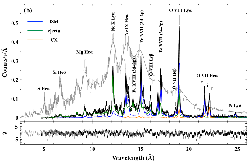
Figure 2 shows MOS1 and combined RGS12 spectra of N49. Prominent lines are detected at 12 Å (Ne X Ly), 13.5 Å (Ne IX He), 15 Å (Fe XVII L; 3d–2p), 16 Å (O VIII Ly), 17 Å (Fe XVII L; 3s–2p), 20 Å (O VII He, O VIII Ly), 22 Å (O VII He). We applied a two-component nonequilibrium ionization (NEI) model (neij; Kaastra & Jansen, 1993) absorbed by neutral gas to the spectra. The NEI model consists of emissions from the overionized hot ejecta and an ionizing cool component originating from the swept-up ISM (Uchida et al., 2015). Although SGR 052666 cannot be spatially resolved with the RGS, according to the result of Uchida et al. (2015), the emission is negligible compared to that from N49 in the energy band covered by the RGS (0.3–2.0 keV).
Free parameters of the NEI components include the electron temperature (), ionization time scale (, where and are the electron number density and the elapsed time since shock heating or rapid cooling, respectively), and emission measure (). In addition to these parameters, the abundances of O (=N=C), Ne, Mg, Si, S, Ar, and Fe (=Ni) of the ejecta were set free. The neij model has another parameter , which represents an initial temperature before a rapid cooling or a shock heating of the plasma. Uchida et al. (2015) determined for the ejecta component mainly from the ionization state of the Fe K emission at 6.6 keV. Since the line centroid is out of the wavelength band of the RGS data, we fixed of the ejecta component at 11 keV based on Uchida et al. (2015). On the other hand, the of the ISM component is fixed at .
Figure 2 (a) shows the result of the spectral fitting with the two-component NEI model (hereafter, NEI model). The best-fit parameters are listed in Table 1. The model well reproduces the overall MOS spectrum; the best-fit parameters of and of the ejecta component are consistent with those obtained by Uchida et al. (2015). Focusing on the RGS spectrum in Figure 3, however, we found discrepancies between the model and the data especially around the O VII triplet, O VIII Ly, and Fe XVII L series.
We first focus on the O VII He line, more specifically on its G-ratio (, where , , and are intensities of the forbidden, intercombination, and resonance lines, respectively. The G-ratio of the O VII He line strongly depends on as presented in Figure 4. We assume here that the emitting plasma is in an ionizing state since most of the O VII He line emission of N49 is attributed to the shocked ISM (Figure 2 (a)). Fitting with four Gaussians, we estimated the G-ratio of the O VII He line observed in N49, which is plotted in Figure 4. The observed G-ratio obviously requires an unreasonably low () with any reasonable range of , indicating necessity of some physical process to enhance the G-ratio.


Charge exchange (CX) is one of the possible processes to make the G-ratio higher. Recent X-ray spectroscopy studies with gratings found enhanced ratios of O VII in Puppis A (Katsuda et al., 2012), and the Cygnus Loop (Uchida et al., 2019). They claimed that the anomalous line ratios are explained by CX X-ray emission. As suggested by Uchida et al. (2019), the CX emission can be enhanced particularly in a region where a shock is interacting with dense gas. CX is therefore promising in the case of N49 since it is interacting with surrounding molecular clouds (Yamane et al., 2018). We thus added a CX model (Gu et al., 2016a) to the NEI model. All the abundances and for the CX component were coupled to those of the ISM component. The collision velocity (i.e. shock velocity) was allowed to vary. We assumed a multiple collision case in which an ion continuously undergoes CX until it becomes neutral. The best-fit “NEICX” model is displayed in Figure 2 (b), and the parameters are listed in Table 1. Although the addition of the CX component improves the residuals at the O VII triplet, the discrepancies still remain around O VIII Ly and Fe XVII L series (Figure 3). Therefore, we conclude that the NEI + CX model is insufficient to describe the spectrum of N49.
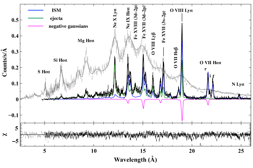
RS is another possible process that would be responsible for the enhanced G-ratio. If photons of the resonance line are scattered off the line of sight due to RS, observed would become lower and the G-ratio would be enhanced. The observed high Fe XVII (3s–2p)/(3d–2p) and O VIII Ly/ ratios can also be caused by RS, as pointed out by previous studies (e.g., Xu et al., 2002; Hitomi Collaboration, 2018). To quantify the contribution of the scattering effect, we added negative Gaussians at wavelengths where lines of the ISM component are prominent in the best-fit NEI model: the O VII He intercombination, O VII He resonance, O VII He, O VIII Ly, O VIII Ly, Fe XVII L, and Ne IX He resonance lines. Since the oscillator strengths of the O VII and Ne IX forbidden lines are several orders of magnitude smaller than those of the other lines, we assume that the scattering effect is negligible for the forbidden lines. The free parameters of the NEI components are the electron temperature (), ionization time scale (), emission measure (). The abundances of O (=N=C), Ne, and Fe (=Ni) of the ejecta were set free and the abundances of Mg, Si, S, and Ar were fixed to the values obtained in the NEI model fit. The best-fit “” model is displayed in Figure 5 and the best-fit parameters are listed in Table 1.
| Line | Transition | Line Centroid ()aaTaken from SPEX. | Transmission FactorbbCalculated from the best-fit parameters of the “” model. |
|---|---|---|---|
| Ne IX He | 13.45 | ||
| Fe XVII L | 15.02 | ||
| Fe XVII L | 15.26 | ||
| O VIII Ly | 16.01 | ||
| Fe XVII L | 16.78 | ||
| Fe XVII L | 17.05 | ||
| O VII He | 18.63 | ||
| O VIII Ly | 18.97 | ||
| O VII He(r) | 21.60 | ||
| O VII He(i) | 21.81 |
4 Discussion
We compare transmission factors estimated based on the result from the “” model fit with those expected for RS. The transmission factor is defined as
| (1) |
where is the total number of photons emitted by the plasma, and is the number of photons scattered out of our line of sight. We can derive for each line from the data, given that the best-fit normalizations of the negative Gaussians and the line intensities of the ISM component correspond to and , respectively. The transmission factors derived from the data are listed in Table 2.
Referring to Kaastra & Mewe (1995), we calculate the transmission factors in a case where RS effectively occurs. Under the slab approximation as a simple geometrical model of the SNR rim, Kaastra & Mewe (1995) used a single-scattering treatment where a photon completely escapes from the line of sight at every scattering event. As shown by Park et al. (2003), the ISM plasma of N49 has a particularly bright emission at the southeastern rim. Assuming that the RS occurs dominantly at the southeastern rim, we adopt the same assumption as Kaastra & Mewe (1995). Then, the transmission factor is written as
| (2) |
where is the optical depth of the ISM plasma (Kastner & Kastner, 1990). The optical depth at the line centroid is given by Kaastra & Mewe (1995) as
| (3) |
where is the oscillator strength of the line, is the line centroid energy in eV, is the hydrogen column density in , is the number density of the ion, is the number density of the element, is the atomic weight of the ion, is the ion temperature in keV, and is the micro-turbulence velocity in units of . We assumed a thermal equilibrium between all ions and electrons and neglected the micro-turbulence velocity. The oscillator strengths and ion fractions for each element were taken from SPEX. In our case, the absorption column density () is the only free parameter.
In Figure 6, we compare the transmission factors estimated from the data and those calculated with equation (2). They are roughly consistent if is (3.0–10), which corresponds to a plasma depth of (10–34) pc. Since the plasma depth is comparable to the diameter of N49, pc, the result supports that RS occurs at the rim of N49. We note that we would underestimate the O abundance by about a factor of 1.8 if we do not take into account the RS effect (Table 1). This demonstrates the importance of RS in measuring elemental abundances as already pointed out by, e.g., Kaastra & Mewe (1995) and Miyata et al. (2008).

In Figure 6, we found that O VIII Ly requires a higher column density than the other lines. A possible explanation would be that RS occurs also in the Galactic Halo (GH), as proposed by Gu et al. (2016b). According to Nakashima et al. (2018), GH spectra are represented by a collisional ionization equilibrium (CIE) plasma model with keV. Since such a plasma has a larger optical depth for the O VIII Ly line than that of the O VII He resonance line, the GH should selectively reduce the intensity of O VIII Ly. We applied the CIE absorption model, hot (de Plaa et al., 2004; Steenbrugge et al., 2005), to the model. The electron temperature and Fe abundance of the hot model are fixed to 0.26 keV and 0.56 solar, respectively (the other elemental abundances are fixed to the solar values), by referring to Nakashima et al. (2018). We found that the discrepancy cannot be reduced with the model, where the transmission factors of O VIII Ly and O VII He are calculated to be and , respectively.
The cause of the observed high O VIII Ly/ ratio (the measured value is 0.18 as an upper limit) is not clear. Uncertainties in the model of the Fe-L lines (e.g., Gu et al., 2019) might partially explain the result since O VIII Ly overlaps with the Fe XVIII L line. Another possibility to explain the high O VIII Ly/ ratio is an effect related to RS. As discussed by Chevalier et al. (1980), Ly can be converted to H by a - transition in a collisionless shock through RS. However, this is less plausible because this effect reduces the intensity of Ly rather than that of Ly. RS by the ejecta may selectively reduce Ly, which we did not take into account in our analysis. We will be able to evaluate the ejecta contribution by measuring the intensity ratio of the emission lines in Fe K, which originates only from the ejecta (e.g., Yamaguchi et al., 2014; Uchida et al., 2015). Since Fe K is out of the wavelength band of the RGS, further observations with X-ray microcalorimeters (e.g., Kelley et al., 2016) is required to clarify this point.
5 Conclusions
We analyzed a high resolution X-ray grating spectrum of LMC SNR N49 obtained with the RGS aboard XMM-Newton. We found that the G-ratio of O VII He is significantly higher than that expected for a thin thermal plasma emission. The ratios of Fe XVII L (3s–2p)/(3d–2p) and O VIII Ly/ also show large residuals from the model. While an extra CX component well reproduces the G-ratio of the O VII He triplet, the residuals around Fe XVII L and O VIII Ly still remain. On the other hand, RS can fairly reproduce the RGS spectrum. We estimated the optical depth for the RS from the intensities of the scattered lines and found that the depth is roughly consistent with the size of N49. Our results indicate that RS has a particularly strong effect on the measurement of oxygen abundance. As demonstrated by Hitomi Collaboration (2018) with the X-ray microcalorimeter SXS aboard Hitomi (Kelley et al., 2016), future missions such as the X-Ray Imaging and Spectroscopy Mission (XRISM; Tashiro et al., 2018) and the Advanced Telescope for High ENergy Astrophysics (Athena; Nandra et al., 2013) will provide useful means for further studying the effects of RS in SNRs.
References
- Banas et al. (1997) Banas, K. R., Hughes, J. P., Bronfman, L., et al. 1997, ApJ, 480, 607
- Broersen et al. (2011) Broersen, S., Vink, J., Kaastra, J., et al. 2011, A&A, 535, A11
- Cash (1979) Cash, W. 1979, ApJ, 228, 939
- Chevalier et al. (1980) Chevalier, R. A., Kirshner, R. P., & Raymond, J. C. 1980, ApJ, 235, 186
- Cline et al. (1982) Cline, T. L., Desai, U. D., Teegarden, B. J., et al. 1982, ApJ, 255, L45
- den Herder et al. (2001) den Herder, J. W., Brinkman, A. C., Kahn, S. M., et al. 2001, A&A, 365, L7
- de Plaa et al. (2004) de Plaa, J., Kaastra, J. S., Tamura, T., et al. 2004, A&A, 423, 49
- de Plaa et al. (2012) de Plaa, J., Zhuravleva, I., Werner, N., et al. 2012, A&A, 539, A34
- Dickey & Lockman (1990) Dickey, J. M., & Lockman, F. J. 1990, ARA&A, 28, 215
- Gu et al. (2016a) Gu, L., Kaastra, J., & Raassen, A. J. J. 2016, A&A, 588, A52
- Gu et al. (2016b) Gu, L., Mao, J., Costantini, E., et al. 2016, A&A, 594, A78
- Gu et al. (2019) Gu, L., Raassen, A. J. J., Mao, J., et al. 2019, A&A, 627, A51
- Hitomi Collaboration (2018) Hitomi Collaboration, Aharonian, F., Akamatsu, H., et al. 2018, PASJ, 70, 10
- Jansen et al. (2001) Jansen, F., Lumb, D., Altieri, B., et al. 2001, A&A, 365, L1
- Kaastra & Jansen (1993) Kaastra, J. S. & Jansen, F. A. 1993, A&A, 97, 873
- Kaastra & Mewe (1995) Kaastra, J. S., & Mewe, R. 1995, A&A, 302, L13
- Kaastra et al. (1996) Kaastra, J. S., Mewe, R., & Nieuwenhuijzen, H. 1996, UV and X-ray Spectroscopy of Astrophysical and Laboratory Plasmas, 411
- Kaastra (2017) Kaastra, J. S. 2017, A&A, 605, A51
- Kastner & Kastner (1990) Kastner, S. O., & Kastner, R. E. 1990, J. Quant. Spec. Radiat. Transf., 44, 275
- Katsuda et al. (2012) Katsuda, S., Tsunemi, H., Mori, K., et al. 2012, ApJ, 756, 49
- Kelley et al. (2016) Kelley, R. L., Akamatsu, H., Azzarello, P., et al. 2016, Proc. SPIE, 99050V
- Lodders et al. (2009) Lodders, K., Palme, H., & Gail, H.-P. 2009, Landolt Bürnstein, 4B, 712
- Miyata et al. (2008) Miyata, E., Masai, K., & Hughes, J. P. 2008, PASJ, 60, 521
- Nakashima et al. (2018) Nakashima, S., Inoue, Y., Yamasaki, N., et al. 2018, ApJ, 862, 34
- Nandra et al. (2013) Nandra, K., Barret, D., Barcons, X., et al. 2013, arXiv e-prints, arXiv:1306.2307
- Park et al. (2003) Park, S., Burrows, D. N., Garmire, G. P., et al. 2003, ApJ, 586, 210
- Park et al. (2012) Park, S., Hughes, J. P., Slane, P. O., et al. 2012, ApJ, 748, 117
- Pietrzyński et al. (2013) Pietrzyński, G., Graczyk, D., Gieren, W., et al. 2013, Nature, 495, 76
- Rugge & McKenzie (1985) Rugge, H. R., & McKenzie, D. L. 1985, ApJ, 297, 338
- Russell & Dopita (1992) Russell, S. C., & Dopita, M. A. 1992, ApJ, 384, 508
- Sanders et al. (2004) Sanders, J. S., Fabian, A. C., Allen, S. W., et al. 2004, MNRAS, 349, 952
- Schenck et al. (2016) Schenck, A., Park, S., & Post, S. 2016, AJ, 151, 161
- Shigeyama (1998) Shigeyama, T. 1998, ApJ, 497, 587
- Steenbrugge et al. (2005) Steenbrugge, K. C., Kaastra, J. S., Crenshaw, D. M., et al. 2005, A&A, 434, 569
- Strüder et al. (2001) Strüder, L., Briel, U., Dennerl, K., et al. 2001, A&A, 365, L18
- Tashiro et al. (2018) Tashiro, M., Maejima, H., Toda, K., et al. 2018, Proc. SPIE, 1069922
- Turner et al. (2001) Turner, M. J. L., Abbey, A., Arnaud, M., et al. 2001, A&A, 365, L27
- Uchida et al. (2015) Uchida, H., Koyama, K., & Yamaguchi, H. 2015, ApJ, 808, 77
- Uchida et al. (2019) Uchida, H., Katsuda, S., Tsunemi, H., et al. 2019, ApJ, 871, 234
- van der Heyden et al. (2003) van der Heyden, K. J., Bleeker, J. A. M., Kaastra, J. S., et al. 2003, A&A, 406, 141
- Waljeski et al. (1994) Waljeski, K., Moses, D., Dere, K. P., et al. 1994, ApJ, 429, 909
- Xu et al. (2002) Xu, H., Kahn, S. M., Peterson, J. R., et al. 2002, ApJ, 579, 600
- Yamaguchi et al. (2014) Yamaguchi, H., Badenes, C., Petre, R., et al. 2014, ApJ, 785, L27
- Yamane et al. (2018) Yamane, Y., Sano, H., van Loon, J. T., et al. 2018, ApJ, 863, 55