Evidence for the Cross-correlation between Cosmic Microwave Background Polarization Lensing from Polarbear and Cosmic Shear from Subaru Hyper Suprime-Cam

T. Namikawa Department of Applied Mathematics and Theoretical Physics, University of Cambridge, Cambridge CB3 0WA, UK Y. Chinone Department of Physics, University of California, Berkeley, CA 94720, USA Kavli Institute for the Physics and Mathematics of the Universe (Kavli IPMU, WPI), UTIAS, The University of Tokyo, Kashiwa, Chiba 277-8583, Japan Kavli Institute for the Physics and Mathematics of the Universe (WPI), Berkeley Satellite, the University of California, Berkeley 94720, USA H. Miyatake Institite for Advanced Research, Nagoya University, Nagoya, Aichi, 464-8601, Japan Division of Particle and Astrophysical Science, Graduate School of Science, Nagoya University, Nagoya, Aichi, 464-8602, Japan Kavli Institute for the Physics and Mathematics of the Universe (Kavli IPMU, WPI), UTIAS, The University of Tokyo, Kashiwa, Chiba 277-8583, Japan M. Oguri Department of Physics, The University of Tokyo, Tokyo 113-0033, Japan Kavli Institute for the Physics and Mathematics of the Universe (Kavli IPMU, WPI), UTIAS, The University of Tokyo, Kashiwa, Chiba 277-8583, Japan Research Center for the Early Universe, School of Science, The University of Tokyo, Bunkyo-ku, Tokyo 113-0033, Japan R. Takahashi Faculty of Science and Technology, Hirosaki University, 3 Bunkyo-cho, Hirosaki, Aomori 036-8588, Japan A. Kusaka Physics Division, Lawrence Berkeley National Laboratory, Berkeley, CA 94720, USA Department of Physics, The University of Tokyo, Tokyo 113-0033, Japan Kavli Institute for the Physics and Mathematics of the Universe (WPI), Berkeley Satellite, the University of California, Berkeley 94720, USA Research Center for the Early Universe, School of Science, The University of Tokyo, Bunkyo-ku, Tokyo 113-0033, Japan N. Katayama Kavli Institute for the Physics and Mathematics of the Universe (Kavli IPMU, WPI), UTIAS, The University of Tokyo, Kashiwa, Chiba 277-8583, Japan S. Adachi Department of Physics, Kyoto University, Kyoto 606-8502, Japan M. Aguilar Department of Physics and Astronomy, Johns Hopkins University, Baltimore, MD 21218, USA Departamento de Física, FCFM, Universidad de Chile, Blanco Encalada 2008, Santiago, Chile H. Aihara Department of Physics, The University of Tokyo, Tokyo 113-0033, Japan Kavli Institute for the Physics and Mathematics of the Universe (Kavli IPMU, WPI), UTIAS, The University of Tokyo, Kashiwa, Chiba 277-8583, Japan A. Ali Department of Physics, University of California, Berkeley, CA 94720, USA R. Armstrong Lawrence Livermore National Laboratory, Livermore, CA 94551, USA K. Arnold Department of Physics, University of California, San Diego, CA 92093-0424, USA C. Baccigalupi International School for Advanced Studies (SISSA), Via Bonomea 265, 34136, Trieste, Italy Institute for Fundamental Physics of the Universe (IFPU), Via Beirut 2, 34151, Grignano (TS), Italy National Institute for Nuclear Physics, INFN, Sezione di Trieste Via Valerio 2, I-34127, Trieste, Italy D. Barron Department of Physics and Astronomy, University of New Mexico, Albuquerque, NM, 87131, USA D. Beck AstroParticule et Cosmologie (APC), Univ Paris Diderot, CNRS/IN2P3, CEA/Irfu, Obs de Paris, Sorbonne Paris Cité, France S. Beckman Department of Physics, University of California, Berkeley, CA 94720, USA F. Bianchini School of Physics, University of Melbourne, Parkville, VIC 3010, Australia D. Boettger Instituto de Astrofísica and Centro de Astro-Ingeniería, Facultad de Física, Pontificia Universidad Católica de Chile, Av. Vicuña Mackenna 4860, 7820436 Macul, Santiago, Chile J. Borrill Computational Cosmology Center, Lawrence Berkeley National Laboratory, Berkeley, CA 94720, USA Space Sciences Laboratory, University of California, Berkeley, CA 94720, USA K. Cheung Department of Physics, University of California, Berkeley, CA 94720, USA L. Corbett Department of Physics, University of California, Berkeley, CA 94720, USA K. T. Crowley Department of Physics, University of California, Berkeley, CA 94720, USA H. El Bouhargani AstroParticule et Cosmologie (APC), Univ Paris Diderot, CNRS/IN2P3, CEA/Irfu, Obs de Paris, Sorbonne Paris Cité, France T. Elleflot Department of Physics, University of California, San Diego, CA 92093-0424, USA J. Errard AstroParticule et Cosmologie (APC), Univ Paris Diderot, CNRS/IN2P3, CEA/Irfu, Obs de Paris, Sorbonne Paris Cité, France G. Fabbian Department of Physics & Astronomy, University of Sussex, Brighton BN1 9QH, UK C. Feng Department of Physics, University of Illinois at Urbana-Champaign, 1110 W Green St, Urbana, IL, 61801, USA N. Galitzki Department of Physics, University of California, San Diego, CA 92093-0424, USA N. Goeckner-Wald Department of Physics, University of California, Berkeley, CA 94720, USA J. Groh Department of Physics, University of California, Berkeley, CA 94720, USA T. Hamada Astronomical Institute, Graduate School of Science, Tohoku University, Sendai, 980-8578, Japan High Energy Accelerator Research Organization (KEK), Tsukuba, Ibaraki 305-0801, Japan M. Hasegawa High Energy Accelerator Research Organization (KEK), Tsukuba, Ibaraki 305-0801, Japan SOKENDAI (The Graduate University for Advanced Studies), Shonan Village, Hayama, Kanagawa 240-0193, Japan M. Hazumi High Energy Accelerator Research Organization (KEK), Tsukuba, Ibaraki 305-0801, Japan Kavli Institute for the Physics and Mathematics of the Universe (Kavli IPMU, WPI), UTIAS, The University of Tokyo, Kashiwa, Chiba 277-8583, Japan SOKENDAI (The Graduate University for Advanced Studies), Shonan Village, Hayama, Kanagawa 240-0193, Japan Institute of Space and Astronautical Science (ISAS), Japan Aerospace Exploration Agency (JAXA), Sagamihara, Kanagawa 252-0222, Japan C. A. Hill Department of Physics, University of California, Berkeley, CA 94720, USA Physics Division, Lawrence Berkeley National Laboratory, Berkeley, CA 94720, USA L. Howe Department of Physics, University of California, San Diego, CA 92093-0424, USA O. Jeong Department of Physics, University of California, Berkeley, CA 94720, USA D. Kaneko Kavli Institute for the Physics and Mathematics of the Universe (Kavli IPMU, WPI), UTIAS, The University of Tokyo, Kashiwa, Chiba 277-8583, Japan B. Keating Department of Physics, University of California, San Diego, CA 92093-0424, USA A. T. Lee Department of Physics, University of California, Berkeley, CA 94720, USA Physics Division, Lawrence Berkeley National Laboratory, Berkeley, CA 94720, USA Radio Astronomy Laboratory, University of California, Berkeley, CA 94720, USA D. Leon Department of Physics, University of California, San Diego, CA 92093-0424, USA E. Linder Space Sciences Laboratory, University of California, Berkeley, CA 94720, USA Physics Division, Lawrence Berkeley National Laboratory, Berkeley, CA 94720, USA L. N. Lowry Department of Physics, University of California, San Diego, CA 92093-0424, USA A. Mangu Department of Physics, University of California, Berkeley, CA 94720, USA Physics Division, Lawrence Berkeley National Laboratory, Berkeley, CA 94720, USA F. Matsuda Kavli Institute for the Physics and Mathematics of the Universe (Kavli IPMU, WPI), UTIAS, The University of Tokyo, Kashiwa, Chiba 277-8583, Japan Y. Minami High Energy Accelerator Research Organization (KEK), Tsukuba, Ibaraki 305-0801, Japan S. Miyazaki National Astronomical Observatory of Japan, Mitaka, Tokyo 181-8588, Japan H. Murayama Kavli Institute for the Physics and Mathematics of the Universe (Kavli IPMU, WPI), UTIAS, The University of Tokyo, Kashiwa, Chiba 277-8583, Japan Department of Physics, University of California, Berkeley, CA 94720, USA M. Navaroli Department of Physics, University of California, San Diego, CA 92093-0424, USA H. Nishino High Energy Accelerator Research Organization (KEK), Tsukuba, Ibaraki 305-0801, Japan A. J. Nishizawa Institite for Advanced Research, Nagoya University, Nagoya, Aichi, 464-8601, Japan A. T. P. Pham School of Physics, University of Melbourne, Parkville, VIC 3010, Australia D. Poletti International School for Advanced Studies (SISSA), Via Bonomea 265, 34136, Trieste, Italy Institute for Fundamental Physics of the Universe (IFPU), Via Beirut 2, 34151, Grignano (TS), Italy The National Institute for Nuclear Physics, INFN, Sezione di Trieste Via Valerio 2, I-34127, Trieste, Italy G. Puglisi Department of Physics, Stanford University, Stanford, CA, 94305, USA C. L. Reichardt School of Physics, University of Melbourne, Parkville, VIC 3010, Australia B. D. Sherwin Department of Applied Mathematics and Theoretical Physics, University of Cambridge, Cambridge CB3 0WA, UK Kavli Institute for Cosmology Cambridge, Cambridge CB3 OHA, UK M. Silva-Feaver Department of Physics, University of California, San Diego, CA 92093-0424, USA P. Siritanasak Department of Physics, University of California, San Diego, CA 92093-0424, USA J. S. Speagle Center for Astrophysics

|

Harvard & Smithsonian, Cambridge MA 02138, USA R. Stompor AstroParticule et Cosmologie (APC), Univ Paris Diderot, CNRS/IN2P3, CEA/Irfu, Obs de Paris, Sorbonne Paris Cité, France A. Suzuki Physics Division, Lawrence Berkeley National Laboratory, Berkeley, CA 94720, USA P. J. Tait Subaru Telescope, National Astronomical Observatory of Japan, Hilo, HI 96720, USA O. Tajima Department of Physics, Kyoto University, Kyoto 606-8502, Japan High Energy Accelerator Research Organization (KEK), Tsukuba, Ibaraki 305-0801, Japan M. Takada Kavli Institute for the Physics and Mathematics of the Universe (Kavli IPMU, WPI), UTIAS, The University of Tokyo, Kashiwa, Chiba 277-8583, Japan S. Takakura Kavli Institute for the Physics and Mathematics of the Universe (Kavli IPMU, WPI), UTIAS, The University of Tokyo, Kashiwa, Chiba 277-8583, Japan S. Takatori SOKENDAI (The Graduate University for Advanced Studies), Shonan Village, Hayama, Kanagawa 240-0193, Japan High Energy Accelerator Research Organization (KEK), Tsukuba, Ibaraki 305-0801, Japan D. Tanabe SOKENDAI (The Graduate University for Advanced Studies), Shonan Village, Hayama, Kanagawa 240-0193, Japan M. Tanaka National Astronomical Observatory of Japan, Mitaka, Tokyo 181-8588, Japan G. P. Teply Department of Physics, University of California, San Diego, CA 92093-0424, USA C. Tsai Department of Physics, University of California, San Diego, CA 92093-0424, USA C. Vergés AstroParticule et Cosmologie (APC), Univ Paris Diderot, CNRS/IN2P3, CEA/Irfu, Obs de Paris, Sorbonne Paris Cité, France B. Westbrook Radio Astronomy Laboratory, University of California, Berkeley, CA 94720, USA Y. Zhou Department of Physics, University of California, Berkeley, CA 94720, USA

Abstract

We present the first measurement of cross-correlation between the lensing potential, reconstructed from cosmic microwave background (CMB) polarization data, and the cosmic shear field from galaxy shapes. This measurement is made using data from the Polarbear CMB experiment and the Subaru Hyper Suprime-Cam (HSC) survey. By analyzing an 11 deg² overlapping region, we reject the null hypothesis at 3.5 $\sigma$ and constrain the amplitude of the cross-spectrum to $\widehat{A}_{\rm lens}=1.70\pm 0.48$ , where $\widehat{A}_{\rm lens}$ is the amplitude normalized with respect to the Planck 2018 prediction, based on the flat $\Lambda$ cold dark matter cosmology. The first measurement of this cross-spectrum without relying on CMB temperature measurements is possible due to the deep Polarbear map with a noise level of ${\sim}$ 6 $\mathrm{\mu K}$ -arcmin, as well as the deep HSC data with a high galaxy number density of $n_{g}=23\,{\rm arcmin^{-2}}$ . We present a detailed study of the systematics budget to show that residual systematics in our results are negligibly small, which demonstrates the future potential of this cross-correlation technique.

cosmic background radiation — cosmology:observations — gravitational lensing — polarization

1 Introduction

Weak lensing of the cosmic microwave background (CMB) and galaxies, referred to respectively as CMB lensing and cosmic shear, is a very powerful tool for constraining cosmology, as it is sensitive to both the cosmic expansion and the growth of the large-scale structure (e.g., Kilbinger 2015; Matilla et al. 2017). Furthermore, weak lensing directly probes the gravitational potential of the large-scale structure that is dominated by dark matter, and is therefore immune to the galaxy bias uncertainty.

The constraining power of CMB lensing and cosmic shear on cosmological parameters, such as the mass fluctuation amplitude $\sigma_{8}$ and matter density $\Omega_{m}$ , can be enhanced by combining these two measurements (e.g., Planck Collaboration: N. Aghanim et al. 2018a and references therein). In the near future, properties of dark energy (or gravity theories), dark matter, and neutrinos will be tightly constrained by such cross-correlation measurements (see e.g., Hu 2002; Abazajian & Dodelson 2003; Acquaviva & Baccigalupi 2006; Hannestad et al. 2006; Namikawa et al. 2010; Abazajian et al. 2015). In addition, it has been argued that the cross-correlation between CMB lensing and cosmic shear is important to mitigate instrumental systematics inherent to these measurements (Vallinotto, 2012; Bianchini et al., 2015, 2016; Liu et al., 2016; Schaan et al., 2017; Abbott et al., 2018), as cross-correlation is immune to additive instrumental biases in each lensing measurement. In the cosmic shear analysis, the calibration bias of galaxy shape measurements is one of the main sources of systematic errors, which may also be calibrated by cross-correlation.

The cross-correlation between CMB lensing and cosmic shear has been measured by multiple experimental groups, including the Atacama Cosmology Telescope (ACT), Planck, South Pole Telescope (SPT), Sloan Digital Sky Survey (SDSS), Canada-France-Hawaii Telescope Lensing Survey (CFHTLenS), CFHT Stripe 82 Survey (CS82), Red Cluster Sequence Lensing Survey (RCSLenS), Kilo Degree Survey (KiDS), and Dark Energy Survey (DES) (Hand et al., 2015; Kirk et al., 2016; Liu & Hill, 2015; Singh et al., 2017; Harnois-Déraps et al., 2016, 2017; Omori et al., 2018). In these measurements, however, the sensitivity to CMB lensing is primarily derived from the CMB temperature data.

One of the difficulties we are facing in CMB lensing measurements is contamination from foreground emissions in CMB lensing maps. For instance, one of the goals of future CMB instruments is to validate the shear calibration for the Large Synoptic Survey Telescope (LSST) at the target accuracy of 0.5% (Vallinotto, 2012; Das et al., 2013; Schaan et al., 2017) by cross-correlating CMB lensing maps with the weak lensing map from LSST (Abazajian et al., 2016; The Simons Observatory Collaboration: P. A. R. Ade et al., 2019). Validating the LSST shear calibration requires a high CMB lensing signal-to-noise. Ultimately, this will come from CMB polarization rather than temperature because the $B$ -mode polarization signal is mostly created from lensing while the temperature is dominated by non-lensing contributions. Furthermore, extragalactic foregrounds cause significant biases in temperature-based lensing, which need to be mitigated (Schaan & Ferraro, 2019). One way to achieve the high lensing signal-to-noise needed and overcome the foreground issue is to resort to CMB polarization data for the lensing reconstruction (van Engelen et al., 2014; Schaan et al., 2017).

For the first time, we present the analysis of the cross-correlation between CMB lensing and cosmic shear where the CMB lensing map is reconstructed from polarization information only. This analysis is made possible by combining two deep overlapping surveys: the CMB polarization measurement by the Polarbear experiment (Arnold et al., 2012; Kermish et al., 2012) and the galaxy shape measurement by Subaru Hyper Suprime-Cam (HSC; Aihara et al., 2018a). The Polarbear CMB polarization survey is among the deepest to date, reaching 6 $\mathrm{\mu K}$ -arcmin. The HSC survey is also one of the deepest wide-field optical imaging surveys, with a high galaxy number density of $n_{g}=23\,{\rm arcmin^{-2}}$ for cosmic shear analyses. The deep imaging also results in a relatively high mean redshift of these galaxies ( $z_{\rm mean}=1.0$ ), enhancing the overlap of the lensing kernel between CMB lensing and cosmic shear from galaxy shapes. As such, the predicted amplitude of the cross-correlation is higher than those for the Kilo-Degree Survey (Kuijken et al., 2015) and DES (Dark Energy Survey Collaboration et al., 2016). It is worth noting that our result represents the first cross-correlation measurement between HSC cosmic shear and CMB lensing (whether in polarization or temperature).

This paper is organized as follows. In Section 2, we briefly review the theoretical background of CMB lensing and cosmic shear. In Section 3, we describe the data used in the analysis. In Section 4, we summarize the method to measure lensing from the CMB polarization map and the galaxy shape catalog. We also present the results of validation tests. We then present the cross-correlation results in Section 5, and conclude in Section 6.

2 Weak Lensing of CMB and Galaxies

CMB polarization anisotropies are distorted by the gravitational potential of the large-scale structure between the CMB last scattering surface and observer (see Lewis & Challinor 2006; Hanson et al. 2010 for reviews). The effect of weak lensing on the CMB is well-described by a remapping of the CMB anisotropies at the last scattering surface:

\displaystyle[\widetilde{Q}\pm{\rm i}\hskip 0.50003pt\widetilde{U}](\widehat{\bm{n}})=[Q\pm{\rm i}\hskip 0.50003ptU][\widehat{\bm{n}}+\bm{\nabla}\phi(\widehat{\bm{n}})]\,,

(1)

where $\widehat{\bm{n}}$ is the pointing vector on the sky, $Q$ and $U$ ( $\widetilde{Q}$ and $\widetilde{U}$ ) denote the primary unlensed (lensed) Stokes parameters, and $\phi$ is the CMB lensing potential. The CMB lensing convergence, $\kappa\equiv-\bm{\nabla}^{2}\phi/2$ , is obtained by solving the geodesic equation, yielding:

\displaystyle\kappa(\widehat{\bm{n}})=\int_{0}^{\chi_{*}}\!\!\,{\rm d}\chi\,\,\frac{\chi_{*}-\chi}{\chi_{*}\chi}\bm{\nabla}^{2}\Psi(\chi\widehat{\bm{n}},\chi)\,,

(2)

where $\chi$ is the comoving distance, $\chi_{*}$ denoting the comoving distance to the last scattering surface, and $\Psi(\bm{x},\chi)$ is the Weyl potential. We assume a flat universe, as we will throughout this paper. The convergence map can be reconstructed from observed CMB maps via mode coupling in CMB anisotropies induced by lensing (Hu & Okamoto, 2002; Okamoto & Hu, 2002).

Lensing also distorts shapes of galaxy images in a galaxy survey. We can statistically measure the lensing distortion to the galaxy shapes, or the so-called shear, by correlating ellipticities of galaxy images (see Bartelmann & Schneider 2001; Munshi et al. 2008; Kilbinger 2015 for reviews). The shear field, $\gamma_{1}(\widehat{\bm{n}})$ and $\gamma_{2}(\widehat{\bm{n}})$ , estimated from galaxy ellipticities, is a spin- $2$ field, and can be transformed to rotationally invariant quantities, the so-called $E$ - and $B$ -mode shear fields, $\gamma^{E}$ and $\gamma^{B}$ , via the spin-2 transformation. Similar to the convergence field in Eq. (2), the $E$ -mode shear field is related to the gravitational potential of the large-scale structure, whereas the $B$ -mode shear field is generated by the vector and tensor perturbations, the post-Born correction, and other nonlinear effects (Cooray & Hu 2002; Dodelson et al. 2003; Cooray et al. 2005; Yamauchi et al. 2013). The $B$ -mode shear field is therefore expected to be very small and is usually measured as a null test.

In a survey region overlapping a CMB experiment and a galaxy survey, a correlated signal exists between CMB lensing and cosmic shear, as they share some of the same large-scale structure along the line-of-sight. Their cross-spectrum, $C_{L}^{\kappa\gamma^{E}}$ , is of great interest in cosmological analyses, since it is immune to additive instrumental biases inherent in these measurements. The cross-spectrum from the scalar perturbations is given by (e.g., Hu 2000):

	$\displaystyle C_{L}^{\kappa\gamma^{E}}$	$\displaystyle=\frac{2}{\pi}\int\!\!\,{\rm d}k\,\,k^{2}\int_{0}^{\chi_{*}}\!\!\,{\rm d}\chi\,\,\int_{0}^{\infty}\!\!\,{\rm d}\chi^{\prime}\,\,$
		$\displaystyle\qquad\times k^{3}P_{\Psi}(k,\chi,\chi^{\prime})S_{L}^{\kappa}(k,\chi)S_{L}^{\gamma^{E}}(k,\chi^{\prime})\,,$		(3)

where $L$ is the angular multipole and $k$ is the Fourier mode of the Weyl potential. The power spectrum of the Weyl potential, $P_{\Psi}(k,\chi,\chi^{\prime})$ , is defined as:

\displaystyle(2\pi)^{3}\delta_{D}^{3}(\bm{k}-\bm{k}^{\prime})P_{\Psi}(k,\chi,\chi^{\prime})=\langle{\Psi_{\bm{k}}(\chi)\Psi^{*}_{\bm{k}^{\prime}}(\chi^{\prime})}\rangle\,,

(4)

where $\delta_{D}^{3}$ is the three-dimensional delta function, $\langle{\cdots}\rangle$ denoting the ensemble average, and $\Psi_{\bm{k}}(\chi)$ is the three-dimensional Fourier transform of the Weyl potential. The dimensionless source functions, $S_{L}^{\kappa}(k,\chi)$ and $S_{L}^{\gamma^{E}}(k,\chi)$ , are given by:

	$\displaystyle S_{L}^{\kappa}(k,\chi)$	$\displaystyle=L(L+1)\frac{j_{L}(k\chi)}{k\chi}\frac{\chi_{}-\chi}{\chi_{}}\,,$		(5)
	$\displaystyle S_{L}^{\gamma^{E}}(k,\chi)$	$\displaystyle=\sqrt{\frac{(L+2)!}{(L-2)!}}\frac{j_{L}(k\chi)}{k\chi}\int_{\chi}^{\infty}\!\!\,{\rm d}\chi^{\prime\prime}\,\,\frac{n(\chi^{\prime\prime})}{\bar{n}}\frac{\chi^{\prime\prime}-\chi}{\chi^{\prime\prime}}\,,$		(6)

where $j_{L}(k\chi)$ is the spherical Bessel function, $n(\chi)$ is the number density distribution of galaxies as a function of the comoving distance (see below), and $\bar{n}$ is the average number density of galaxies per square arcminute. We use CAMB¹¹1Code for Anisotropies in the Microwave Background (https://camb.info/)(Lewis et al., 2000) to compute the cross-spectrum defined above. Here we use the fitting formula for the nonlinear matter power spectrum obtained in Takahashi et al. (2012), and employ the actual redshift distribution shown later.

3 Data and Observations

3.1 Polarbear

Polarbear is a CMB experiment that has been operating on the 2.5 m Huan Tran Telescope at the James Ax Observatory at an elevation of 5,190 m, in the Atacama Desert in Chile since Jan 2012. The Polarbear receiver has an array of 1,274 transition edge sensors (TES) cooled to 0.3 K, observing the sky through lenslet-coupled double-slot dipole antennas at 150 GHz. More details on the receiver and telescope can be found in Arnold et al. (2012) and Kermish et al. (2012).

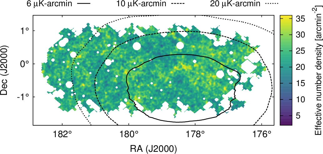
Our analysis uses data from an 11 ${\rm deg}^{2}$ Polarbear contiguous field that overlaps the HSC WIDE survey (see Figure 1). The field is centered at (RA, Dec)=(11^h53^m0^s, $-0$ ^∘30′) and was observed with Polarbear for about 19 months, from 2012 to 2014. The approximate noise level of the polarization map is 6 $\mathrm{\mu K}$ -arcmin.

The observation and map-making are described in The Polarbear Collaboration: P. A. R. Ade et al. (2017) (hereafter PB17). Here, we use a map generated by their pipeline-A algorithm. Based on the MASTER method (Hivon et al., 2002), the pipeline-A performs low/high-pass and azimuthal filters to remove atmospheric noise and ground pickup, respectively, prior to map-making. We construct an apodization window , $W_{\rm cmb}$ , from a smoothed inverse variance weight of the Polarbear map as shown in Figure 1. Map pixels within 3′ of point sources are also masked. In order to reduce the $E$ - $B$ leakage, the apodization edges are modified, using the $C^{2}$ taper described in Grain et al. (2009). We multiply the $Q$ / $U$ maps with this apodization window and compute the pure $B$ - and $E$ -modes (Smith, 2006).

Refer to caption — Figure 1: The overlapping sky coverage of Polarbear and HSC maps in this work. Contours show the noise level of the Polarbear CMB polarization maps. The color map shows the effective number density of the HSC galaxy catalog.

3.2 HSC

HSC is a wide-field optical imager mounted at the prime focus of the Subaru Telescope at the summit of Mauna Kea (Miyazaki et al., 2018; Komiyama et al., 2018). HSC offers a wide field-of-view (1.77 deg²), with superb image quality, and routinely $<0\farcs 6$ seeing sizes, and a fast, deep imaging capability due to the large primary mirror (8.2 m in diameter). As a result, HSC is one of the best instruments for weak lensing surveys. To take advantage of its survey capability, HSC started a wide, deep galaxy imaging survey in 2014 as the Subaru Strategic Program (SSP; Aihara et al., 2018a), which includes the WIDE layer, aiming to cover 1,400 deg² of the sky down to $i_{\rm lim}\sim$ 26 (point source detection at 5 $\sigma$ ) in five broad bands ( $grizy$ ).

In this paper, we use galaxies from the first-year HSC galaxy shape catalog (Mandelbaum et al., 2018a) for the cross-correlation study. The shape catalog includes galaxies with their $i$ -band magnitudes, which are brighter than 24.5, after correcting for the Galactic extinction (Schlegel et al., 1998). The shapes of these galaxies are estimated on coadded $i$ -band images with the re-Gaussianization method (Hirata & Seljak, 2003); this method was extensively used in the SDSS, as its systematics are well-understood (Mandelbaum et al., 2005; Reyes et al., 2012; Mandelbaum et al., 2013). The shape catalog contains calibration factors for each galaxy derived from image simulations (Mandelbaum et al., 2018b), and generated by GalSim (Rowe et al., 2015): the shear multiplicative bias $m$ (shared among two shear components) and the additive bias for each shear component $c_{1}$ and $c_{2}$ . The following quantities are also calibrated against the image simulations: the intrinsic shape noise $e_{\rm rms}$ , the estimated measurement noise ${\sigma_{e}}$ , and the inverse-variance weight from both $e_{\rm rms}$ and ${\sigma_{e}}$ . Note that we use an updated version of the shape catalog from the one originally presented in Mandelbaum et al. (2018a), where bright stars are masked with the new “Arcturus” star catalog (Coupon et al., 2018), which is improved in comparison to the old “Sirius” catalog (see Mandelbaum et al., 2018a; Coupon et al., 2018, for detailed discussions).

In this paper, we use the $13.3$ deg² HSC WIDE12H field, as it overlaps with the Polarbear survey. The WIDE12H field is one of six distinct fields observed from March 2014 to April 2016 for about 90 nights in total, which is a slight extension of the Public Data Release 1 (Aihara et al., 2018b). The HSC data are reduced by the HSC pipeline (Bosch et al., 2018). The weighted number density of source galaxies in this field is 23.4 arcmin^-2 and its median (mean) redshift (see below) is $z_{\rm median}=0.88$ ( $z_{\rm mean}=1.0$ ). Figure 1 shows the overlapping sky coverage of the Polarbear and HSC data in this paper. The overlapping sky coverage is 11.1 ${\rm deg}^{2}$ , where the noise level of the Polarbear polarization measurement is smaller than 20 $\mu$ K-arcmin.

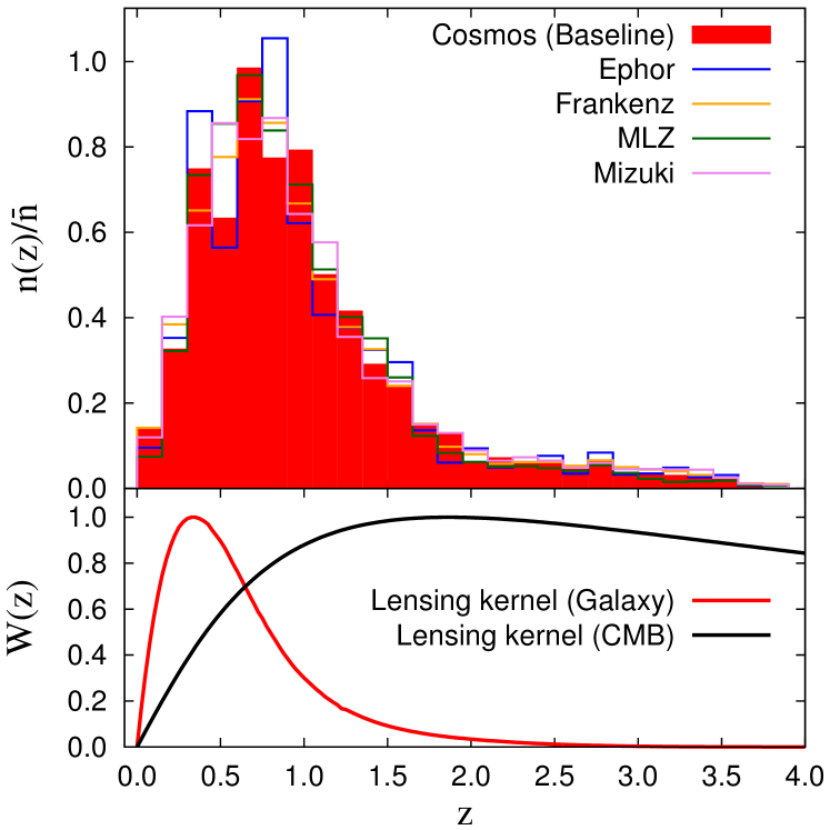
For the baseline analysis, we use the redshift distribution of the source galaxies estimated from COSMOS 30-band photometric redshifts (Ilbert et al., 2009), which were estimated for galaxies in the COSMOS field, using 30 photometric bands spanning from ultraviolet to mid-infrared. We reweight the redshift distribution of the COSMOS 30-band photometric redshift sample to adjust it to match our source galaxy sample on a self-organizing map created with four colors of HSC (More et al. in prep., see also Miyatake et al. 2019; Hikage et al. 2019). To test the robustness of this result, we compare the one predicated on this baseline redshift distribution, with those obtained using several photometric redshift estimations (based solely on the four HSC colors): “Ephor,” “Frankenz,” “MLZ,” and “Mizuki” in the WIDE12H field (Tanaka et al., 2018). For each case, the total redshift distribution of the source galaxy sample is obtained by stacking the photometric redshift probability distribution function of each galaxy in this paper. Figure 2 shows the redshift distributions of the source galaxies derived from these methods. The comparison of the lensing kernels between the HSC galaxies and CMB, as shown in the figure, suggests that we typically probe the large-scale structure at $z\sim 0.5\text{--}1$ by our cross-correlation analysis.

In all analyses of the HSC data, we use magnitudes corrected for the Galactic extinction. Therefore, we do not expect any cross-correlation between the dust contamination in our CMB and optical data. Although there might be a residual effect due to an imperfect correction of the Galactic extinction on galaxy magnitudes, for example, it is currently poorly understood and expected to be small compared to the noise level of our cross-correlation signal.

3.3 Simulated Data

We create simulated data to estimate the covariance and to perform validation tests. The mock simulations are based on the all-sky ray-tracing simulations generated by Takahashi et al. (2017), and in each one, they generate both CMB and galaxy lensing signals. We then add realistic noise, following noise properties of each survey as described below. From an all-sky ray-tracing simulation, we randomly cut out areas corresponding to the HSC WIDE12H geometry to create many independent realizations. In total, we generate 100 WIDE12H field realizations from the single all-sky realization. Takahashi et al. (2017) confirmed that such non-overlapping regions taken from a single full-sky map are mutually independent.

We add HSC source galaxies to the ray-tracing simulation following the prescription described in Oguri et al. (2018). We start with the real HSC galaxy catalog in order to simulate survey features such as the survey geometry, the inhomogeneity of the galaxy distribution, and galaxy properties including redshifts , which is randomly drawn from the photometric redshift probability density function of each galaxy estimated by MLZ, and intrinsic shapes. The galaxy positions and redshifts are maintained unchanged but their shapes are randomly rotated to remove the weak lensing shear associated with the real data. By doing so, we can also preserve the shot-noise originating from galaxy intrinsic shapes and pixel noises. We then add the simulated cosmic shear field derived from the ray-tracing simulation to each rotated galaxy shape to create a mock catalog.

For CMB, we generate Monte Carlo (MC) simulations, having similar properties to the Polarbear data, by scanning a lensed CMB $Q$ / $U$ polarization map from the all-sky simulation described above. We then add a random noise to the simulated detector timestream, where the variance of the noise is equivalent to that measured from the data.

4 Lensing Reconstruction and Cross-correlation Methods

In this section, we describe our method for the cross-correlation analysis. The lensing reconstruction and cross-spectrum estimator are described in Section 4.1. We also describe the validation tests for Polarbear CMB lensing in Section 4.2 and HSC cosmic shear in Section 4.3.

Since the auto spectra of CMB lensing and cosmic shear are validated in PB17 and Hikage et al. (2019), Oguri et al. (2018), and Mandelbaum et al. (2018a), respectively, we focus here on the validation tests for the cross-spectrum between CMB lensing and cosmic shear.

4.1 Estimators

4.1.1 CMB Lensing Convergence

Reconstruction methods of the CMB lensing convergence have been developed by multiple CMB collaborations, including ACT (Sherwin et al., 2017), BICEP/Keck Array (Bicep2 / Keck Array Collaboration, 2016), Planck (Planck Collaboration: N. Aghanim et al., 2018a), Polarbear (The Polarbear Collaboration: P. A. R. Ade et al., 2014a, b), and SPT (van Engelen et al., 2012; Story et al., 2015).

In this paper, we first apply the diagonal inverse-variance filter defined in Eq. (17) of Bicep2 / Keck Array Collaboration (2016) to the $E$ - and $B$ -modes obtained in Section 3.1. The unnormalized quadratic estimator for the lensing convergence is obtained by convolving two CMB $E$ -modes ( $EE$ estimator) or $E$ - and $B$ -modes ( $EB$ estimator) (Hu & Okamoto, 2002):

\displaystyle\overline{\kappa}^{XY}_{\bm{L}}

\displaystyle=\int\!\!\frac{\,{\rm d}^{2}\bm{\ell}\,}{(2\pi)^{2}}\,w^{XY}_{\bm{\ell},\bm{L}}\overline{X}_{\bm{\ell}}\overline{Y}_{\bm{L}-\bm{\ell}}\,,

(7)

where $\overline{X}$ and $\overline{Y}$ are either $E$ - or $B$ -modes filtered by the diagonal inverse-variance. The weight functions are given by Hu & Okamoto (2002):

	$\displaystyle w^{EE}_{\bm{\ell},\bm{L}}$	$\displaystyle=[C^{EE}_{\ell}\bm{L}\cdot\bm{\ell}+C^{EE}_{\|\bm{L}-\bm{\ell}\|}(\bm{L}-\bm{\ell})\cdot\bm{L}]\cos 2(\varphi_{\bm{\ell}}-\varphi_{\bm{L}-\bm{\ell}})\,,$		(8)
	$\displaystyle w^{EB}_{\bm{\ell},\bm{L}}$	$\displaystyle=C^{EE}_{\ell}\bm{L}\cdot\bm{\ell}\sin 2(\varphi_{\bm{\ell}}-\varphi_{\bm{L}-\bm{\ell}})\,,$		(9)

where $C^{EE}_{\ell}$ is the lensed CMB $E$ -mode spectrum (Hanson et al., 2011), and $\varphi_{\bm{\ell}}$ is the angle between $\bm{\ell}$ and the $x$ -axis. We use the CMB multipole range of $500\leq\ell\leq 2700$ in our baseline analysis. The larger multipoles are removed to avoid beam uncertainties and systematic biases due to astrophysical foregrounds such as radio sources (van Engelen et al., 2014). The multipoles at $\ell<500$ is not used because they are not validated in PB17. We then obtain our best estimate of the CMB lensing convergence as:

\displaystyle\widehat{\kappa}^{XY}_{\bm{L}}=A^{XY}_{L}(\overline{\kappa}^{XY}_{\bm{L}}-\langle{\overline{\kappa}^{XY}_{\bm{L}}}\rangle)\,.

(10)

The mean field, $\langle{\overline{\kappa}^{XY}_{\bm{L}}}\rangle$ , is sourced from, for example, masking, inhomogeneous map noise, point sources, and the asymmetric beam (Hanson et al., 2011; Namikawa et al., 2013), and is non-zero, even if we use polarization-only estimators (e.g., Planck Collaboration: P. A. R. Ade et al. 2014). We estimate the mean-field bias from simulation, and the bias is found to be much smaller than the lensing signal in our case. The normalization, $A^{XY}_{L}$ , is computed by following The Polarbear Collaboration: P. A. R. Ade et al. (2014b). Finally, the minimum variance estimator (MV) is obtained by combining the $EE$ and $EB$ estimators (Hu & Okamoto, 2002).

4.1.2 Cosmic Shear

The shear field at a pixel $\widehat{\bm{n}}$ is estimated from the galaxy shape catalog as (Mandelbaum et al., 2018a):

\displaystyle\gamma_{j}(\widehat{\bm{n}})

\displaystyle=\frac{1}{\sum_{i\in g_{\widehat{\bm{n}}}}w_{i}}\frac{1}{1+m}\sum_{i\in g_{\widehat{\bm{n}}}}w_{i}\left[\frac{e_{j,i}}{2R}-c_{j,i}\right]\,,

(11)

where $e_{j,i}$ ( $j=1,2$ ) is the ellipticity of the $i$ -th galaxy, $c_{j,i}$ is the additive bias, $w_{i}$ is the inverse-variance weight, and $\sum_{i\in g_{\widehat{\bm{n}}}}$ is the summation over all galaxies, falling within pixel $\widehat{\bm{n}}$ . The averaged multiplicative bias, $m$ , and the shear responsivity, $R$ , are derived as:

	$\displaystyle m$	$\displaystyle=\frac{\sum_{i\in g_{\rm all}}w_{i}m_{i}}{\sum_{i\in g_{\rm all}}w_{i}}\,,$		(12)
	$\displaystyle R$	$\displaystyle=1-\frac{\sum_{i\in g_{\rm all}}w_{i}e^{2}_{{\rm rms},i}}{\sum_{i\in g_{\rm all}}w_{i}}\,.$		(13)

Here, $m_{i}$ is the multiplicative bias, $\sum_{i\in g_{\rm all}}$ is the summation over all galaxies for the cross-correlation analysis, and $e_{{\rm rms},i}$ is the root-mean square of intrinsic ellipticities. The shear maps, $\gamma_{1}$ and $\gamma_{2}$ , are then multiplied by a window function constructed from the weight, $W_{\rm gal}(\widehat{\bm{n}})=\sum_{i\in g_{\widehat{\bm{n}}}}w_{i}$ , and transformed to $E$ - and $B$ -mode shear fields as:

\displaystyle\gamma^{E}_{\bm{L}}\pm{\rm i}\hskip 0.50003pt\gamma^{B}_{\bm{L}}=\int\!\!\,{\rm d}^{2}\widehat{\bm{n}}\,\,\hskip 1.00006pt{\rm e}^{-{\rm i}\hskip 0.40974pt\bm{L}\cdot\widehat{\bm{n}}}\hskip 1.00006pt{\rm e}^{\pm 2{\rm i}\hskip 0.40974pt\varphi_{\bm{L}}}W_{\rm gal}(\widehat{\bm{n}})[\gamma_{1}\pm{\rm i}\hskip 0.50003pt\gamma_{2}](\widehat{\bm{n}})\,.

(14)

4.1.3 Cross-spectrum

The binned cross-spectrum is obtained by cross-correlating the CMB lensing convergence and the $E$ -mode shear field derived above. Since the cross-spectrum is a correlation between two CMB and one cosmic shear maps, the cross-spectrum is further divided by $\int{\rm d}^{2}\widehat{\bm{n}}\,W^{2}_{\rm cmb}(\widehat{\bm{n}})W_{\rm gal}(\widehat{\bm{n}})$ to correct the normalization due to the apodization window, where $W_{\rm cmb}$ is the CMB apodization window defined in Section 3.1. The number of multipole bins is $9$ and the multipole range of the output power spectrum is $100\leq L\leq 1900$ . The lower limit of $L$ is set by the size of the survey region, and the higher limit of $L$ is set because signal-to-noise ratios above $L=1900$ are negligibly small. Before unblinding, we confirmed that the measured spectrum from the realistic MC simulation reproduces the input power spectrum within the simulation error.

4.2 Validation Tests: CMB

We describe a suite of data-split null tests and instrumental systematics to validate CMB datasets in the cross-spectrum.

4.2.1 Data-split Null Tests

In order to validate the Polarbear data and analysis in the cross-correlation with the HSC data, we perform a suite of null tests. These validation tests are essentially the extension of those described in PB17 to the cross-correlation, in which we iteratively run the null-test framework until a set of predefined criteria is passed.

For each null test, we reconstruct two lensing maps, $\kappa^{A}$ and $\kappa^{B}$ , one from each data split. The reconstructed lensing maps are then cross-correlated with the HSC shear map to obtain a null spectrum for the difference between the two cross-spectra, $C_{L}^{\kappa^{A}\gamma^{E}}-C_{L}^{\kappa^{B}\gamma^{E}}$ . To evaluate the statistical significance, we repeat the same calculation using the simulated CMB maps, but with the actual HSC shear data.

The null tests are performed for several splits of interest for the Polarbear data, which are identified to be sensitive to various sources of systematic contaminations or miscalibrations. We perform 12 null tests in total, and the correlations among these null tests are noted in the analysis by running the same suite of null tests on noise-only MC simulations. Four tests divide the data by the observation period such as the first season data and the second season data. Three tests target effects that depend on the telescope pointing/scan such as data taken at high or low elevation. Three tests divide based on the proximity of the main or sidelobe beams to the Sun and Moon. Two tests divide the data by focal-plane pixels based on susceptibility to instrumental effects. Details of the 12 null tests are described in The Polarbear Collaboration: P. A. R. Ade et al. (2014c, hereafter PB14) and PB17.

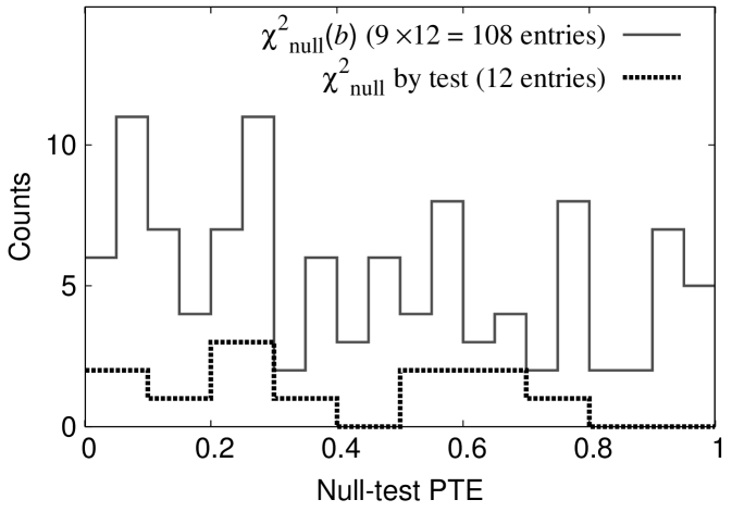
We also adopt the same null-test statistics as defined in PB17. For each band power bin $b$ , we calculate the statistic $\chi_{\rm null}(b)\equiv\hat{C}_{b}^{\rm null}/\sigma_{b}$ , where $\sigma_{b}$ is a MC-based estimate of the standard deviation of the null spectra, and its square $\chi_{\rm null}^{2}(b)$ . The $\chi_{\rm null}(b)$ is sensitive to a systematic bias in the null spectra, whereas the $\chi_{\rm null}^{2}(b)$ is more sensitive to outliers and excess in the variance. In order to investigate possible systematic contaminations or miscalibrations affecting a specific null-test data split, we calculate the sum of the $\chi_{\rm null}^{2}(b)$ over $100\leq L\leq 1900$ (“ $\chi^{2}_{\rm null}$ by test”). We require each set of probability to exceeds (PTEs) from the $\chi_{\rm null}^{2}(b)$ and the $\chi_{\rm null}^{2}$ by test to be consistent with a uniform distribution. We have evaluated it by using a Kolmogorov-Smirnov (KS) test, to be equal to or greater than 0.05. We find these distributions consistent with the uniform distribution. Figure 3 and Table 1 show PTE distributions of $\chi^{2}_{\rm null}(b)$ and $\chi^{2}_{\rm null}$ by test, and the PTEs of the KS test.

Table 1: PTEs from the data-split null tests.

	Type	PTE
	KS test of ${\rm PTE}_{\chi^{2}_{\rm null}(b)}$	0.07
	KS test of ${\rm PTE}_{\chi^{2}_{\rm null}\text{ by test}}$	0.63
(1)	Average of $\chi_{\rm null}(b)$	0.88
(2)	Extreme of $\chi^{2}_{\rm null}(b)$	0.44
(3)	Extreme of $\chi^{2}_{\rm null}$ by test	0.16
(4)	Total $\chi^{2}_{\rm null}$	0.10

In order to search for different manifestations of systematic contaminations, we also create the same test statistics based on these quantities described in PB17. The four test statistics are PTEs from (1) the average value of $\chi_{\rm null}$ , (2) the extreme value of the $\chi^{2}_{\rm null}$ by bin, (3) that by test, and (4) the total $\chi^{2}_{\rm null}$ summed by the 12 null tests. In each case, the result from the data is compared to the result from simulations to calculate PTEs, as Table 1 summarizes the PTEs.

Finally, by comparing the most significant outlier from the four test statistics to those of the MC simulations, we obtain a PTE of 0.24. In all tests, we find no evidence for systematic contaminations or miscalibrations in the Polarbear dataset correlated with the HSC dataset.

4.2.2 Instrumental Systematics

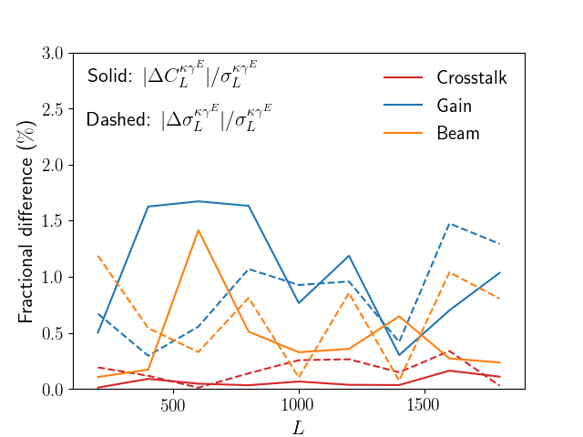
We study the impact of uncertainties in the instrument model of Polarbear on the lensing auto and cross-spectra by producing a simulated signal-only data set in a time domain where the signal is modeled with lensed CMB simulations, obtained by LensPix²²2https://cosmologist.info/lenspix/ with instrumental effects added on the fly. With this simulation setup, systematic errors in auto spectra contains both multiplicative and additive bias in CMB lensing measurement, allowing us to put a conservative upper limit on the multiplicative component. On the other hand, this simulation has zero expectation value in the cross power, while containing fiducial power in each of the CMB and weak lensing maps; this is an appropriate setup for estimating the additive component, whose estimate can depend on the signal power of each map. Here, we investigated six instrumental systematics effects: crosstalk in the multiplexed readout, drift of the gains between two consecutive thermal source calibrator measurements, differential beam ellipticity, differential beam size, relative gain-calibration uncertainty between the two detectors in a focal-plane pixel, and differential pointing between the two detectors in a focal-plane pixel. Details of these systematic effects and systematics simulations are described in PB14 and PB17. These contamination s are found not to bias lensing auto spectrum significantly, putting an upper limit on multiplicative bias. The limit corresponds to $0.6\%$ of fiducial lensing amplitude in the $A_{\rm lens}$ measurement (Polarbear collaboration et al., in prep.).

In order to explicitly check the impact of the instrumental systematics on cross-spectrum, we reconstructed the CMB maps with Polarbear pipeline-A and the corresponding CMB lensing convergence maps from the simulated data set. These maps are cross-correlated with the HSC mock data as described in Section 3.3. Figure 4 shows the impact of the CMB instrumental systematics on the cross-spectra. As expected, all the systematics and their variances are negligibly small, compared to the statistical errors estimated from the MC simulations. Specifically, we find upper limits of ${\sim}1$ % level on the instrumental systematic errors compared to the statistical errors for most cases. We therefore find no evidence for significant contaminations from the CMB instrumental systematics in the cross-correlation analysis. The upper limit corresponds to $1.3\%$ , in terms of $A_{\rm lens}$ , when compared to fiducial amplitude.

While our estimate of the systematics is for the Polarbear instrument, future CMB instruments aim to achieve similar, if not better, levels of systematics. We detect no significant systematic error and the upper limit presented here is dominated by the statistical uncertainty of MC simulations. The upper limit is already comparable to the goals of Simons Observatory and CMB-S4, which calibrate the shear bias of LSST to ${\sim}0.5\%$ accuracy (Schaan et al., 2017; Abazajian et al., 2016; The Simons Observatory Collaboration: P. A. R. Ade et al., 2019).

4.3 Validation Tests: Shear

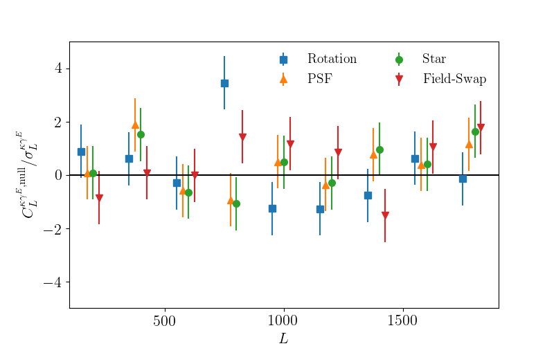
We perform four validation tests for the shear map derived from the HSC data, by cross-correlating the CMB lensing map with the following null test maps, created in the same manner as the real shear map:

•

Rotation: a map from randomly rotated ellipticities of galaxies in the HSC WIDE12H field to remove the cosmic shear signal,
•

Star: a map from ellipticities of stars for reconstructing the Point Spread Function (PSF), again in the HSC WIDE12H field,
•

PSF: a map from PSFs reconstructed at the star position, and
•

Field Swap: a shear map measured in another field, not overlapping with the WIDE12H field.

We expect null signals for all four cases, since these maps do not have any physical correlation with the CMB lensing map.

For the Rotation test, we measure cross-spectra without correcting for multiplicative and additive biases, i.e., we set $m_{i}=0$ and $c_{i}=0$ in Eq. (11). This ignorance of the multiplicative bias does not affect our validation test. For the Star and PSF tests, we measure their cross-power spectra with $w_{i}=1$ , $m_{i}=0$ , $e_{{\rm rms},i}=0$ , and $c_{i}=0$ . The equal weight is derived from the fact that all stars in this test have similar signal-to-noise ratio, which is also the case for PSFs. The zero RMS ellipticity is derived from the fact that stars and PSFs have approximately zero ellipticity, on average.

We estimate the covariance and PTEs as follows. We first generate simulations by randomly rotating ellipticities of galaxies, stars, and PSFs in the real WIDE12H field data for the Rotation, the Star, and the PSF tests, respectively. We then measure cross-spectra in a consistent way with the measurement described above. Based on 100 realizations of the HSC maps with randomly rotated ellipticities, we estimate the covariance and use it to compute PTEs.

For the Field Swap test, we use another patch of the HSC first-year shear catalog, GAMA09H, which is located in RA of ${\sim}9$ h. Since there is no overlap of the footprints between the Polarbear field and the GAMA09H field, there is no cross-correlation between these data. We compute the shear map of the GAMA09H field using the same method as described in Section 4.1 with the calibration of multiplicative and additive bias. In order to estimate the covariance and PTEs, we use the 100 realizations of simulations similar to those described in Section 3.3 but remove to match the GAMA09H area. Note that the mock shear catalogs contain the same calibration bias as in the real HSC shear catalog.

Figure 5 shows the cross-spectra between the HSC null test maps and the real CMB lensing map. The results of these null tests are also summarized in Table 2. We find no evidence for systematic errors from this analysis.

Table 2: Results of the HSC shear null tests.

	$\chi$ -PTE	$\chi^{2}$ -PTE
Rotation	0.52	0.10
Star	0.26	0.43
PSF	0.46	0.49
Field Swap	0.20	0.33

4.4 Blind Analysis

We adopt a blind analysis policy, in which the cross-spectrum is revealed only after the data pass a series of null tests and systematic error checks as described in Section 4.2 and 4.3. For the HSC data, we prepare three shape catalogs with different multiplicative biases, each of which has a different, blinded offset. For details of the blinding strategy, see Hikage et al. (2019). For the Polarbear data, the null tests and the possible sources of instrumental systematic errors are finalized before the cross-spectrum is examined, in order to motivate a comprehensive validation of the dataset and to avoid an observer bias in the analysis.

5 Results

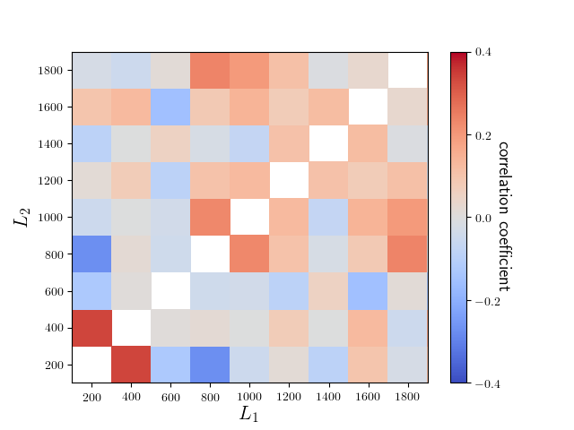
Figure 6 shows the angular cross-spectrum between Polarbear CMB lensing and HSC cosmic shear. We show the cross-spectrum measured spectra using the optimal combination of the $EE$ and $EB$ estimators (MV). Since our CMB $B$ -mode map is very deep, the power spectrum from the $EB$ estimator is less noisy than that from the $EE$ estimator. We also find that the cross-spectrum between the HSC $B$ -mode shear and the CMB lensing convergence is consistent with zero ( $\chi\text{-PTE}$ and $\chi^{2}\text{-PTE}$ of 0.26 and 0.68, respectively) as expected. Figure 7 shows the correlation coefficients among different multipole bins of the cross-spectrum, defined as;

\displaystyle R_{bb^{\prime}}=\frac{{\bm{\mathrm{Cov}}}_{bb^{\prime}}}{\sqrt{{\bm{\mathrm{Cov}}}_{bb}}\sqrt{{\bm{\mathrm{Cov}}}_{b^{\prime}b^{\prime}}}}\,.

(15)

Here, ${\bm{\mathrm{Cov}}}_{bb^{\prime}}=\langle{C_{b}C_{b^{\prime}}}\rangle-\langle{C_{b}}\rangle\langle{C_{b^{\prime}}}\rangle$ is the covariance of the binned cross-power spectrum. The correlation coefficient between the first and second bandpowers is ${\sim}0.4$ , and that between the first and fourth bandpowers is ${\sim}-0.3$ . Most of the correlation coefficients is consistent with zero within statistical uncertainty ( ${\sim}10\%$ ) from the finite number of the MC realizations.

To see the consistency of our cross-spectrum measurement with the Planck $\Lambda$ -dominated cold dark matter ( $\Lambda$ CDM) cosmology, we estimate the amplitude of the cross-spectrum by a weighted mean over multipole bins (Bicep2 / Keck Array Collaboration 2016):

\displaystyle\widehat{A}_{\rm lens}=\frac{\sum_{b}a_{b}A_{b}}{\sum_{b}a_{b}}\,.

(16)

The $A_{b}$ is the relative amplitude of the power spectrum compared with a fiducial power spectrum for the Planck $\Lambda$ CDM cosmology, $C_{b}^{\rm f}$ , i.e., $A_{b}\equiv C_{b}/C_{b}^{\rm f}$ . The weights, $a_{b}$ , are taken from the bandpower covariance as:

\displaystyle a_{b}=\sum_{b^{\prime}}C^{\rm f}_{b}{\bm{\mathrm{Cov}}}_{bb^{\prime}}^{-1}C^{\rm f}_{b^{\prime}}\,.

(17)

The fiducial bandpower values and their covariances, including off-diagonal correlations between different multipole bins, are evaluated from the simulations (see Section 3.3). In our baseline analysis, we assume the $\Lambda$ CDM cosmology with the Planck 2018 best-fit parameters (TT,TE,EE+lowE+lensing).

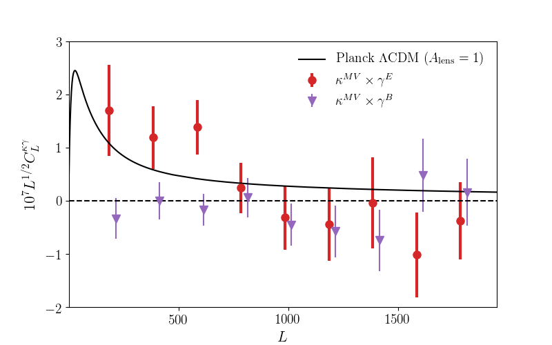
The amplitude estimated from the observed cross-spectrum is $\widehat{A}_{\rm lens}=1.70\pm 0.48$ ,³³3Our simulations assume the WMAP-9 best-fit cosmology, whereas the baseline analysis of the amplitude is measured against the Planck 2018 best-fit cosmology (“TT,TE,EE+lowE+lensing” in Planck Collaboration: N. Aghanim et al. 2018b). This leads to a small change in the mean and scatter of the amplitude parameter. We correct this discrepancy by scaling the simulated cross-spectrum at each realization as $C^{i}_{b}\times(C^{\rm f}_{b}/\langle{C^{i}_{b}}\rangle)$ . The variance of the amplitude of simulations is scaled by a value estimated from analytic calculations of cross-spectra in Planck and WMAP-9 cosmologies, using $n_{g}=23\,{\rm arcmin^{-2}}$ , $e_{\rm rms}=0.4$ , a 6 $\mathrm{\mu K}$ -arcmin CMB white noise, and a $3\farcm 5$ Gaussian beam. corresponding to the detection of a non-zero cross-correlation at 3.5 $\sigma$ significance. Here, the quoted error is the standard deviation of $A_{\rm lens}$ obtained from the MC simulations. The MC error in the covariance changes the cross-spectrum amplitude by only $\Delta\widehat{A}_{\rm lens}=\pm 0.06$ . The high detection significance is in part because of the central value fluctuated high; for a fiducial value of $A_{\rm lens}=1$ , the expected signal-to-noise ratio is $S/N\sim 2$ . The PTE of the spectrum with respect to the fiducial Planck $\Lambda$ CDM cosmology is $66$ %.

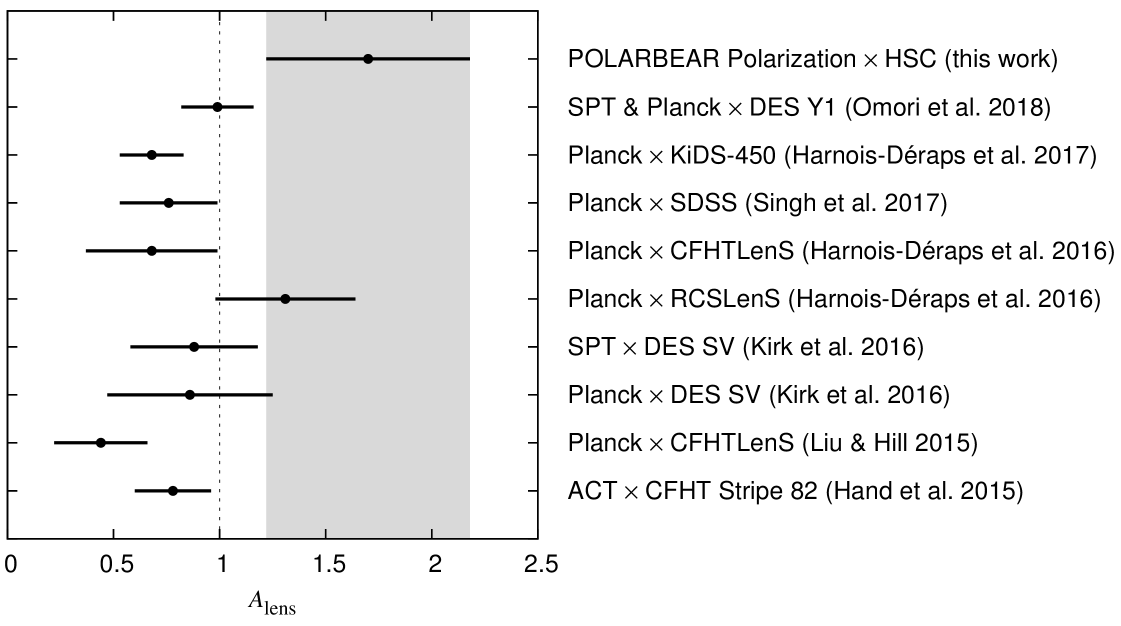
Figure 8 compares the values of $A_{\rm lens}$ and their $1\sigma$ errors among recent cross-correlation studies between CMB lensing and cosmic shear from galaxy shapes. The $\widehat{A}_{\rm lens}$ value obtained is slightly higher than unity but is consistent with the Planck prediction within $2\sigma$ level. Our result also agrees with the previous cross-correlation analyses, although their best-fit values still have a large variation $A_{\rm lens}\simeq 0.4\text{--}1.3$ (e.g., Liu & Hill, 2015; Harnois-Déraps et al., 2016, 2017). It should be noted that in the other cross-correlation studies, CMB lensing signals are dominated by those from the temperature maps, unlike our study, in which we use the polarization map only. In addition, the redshift distributions of source galaxies are different among these measurements.

To check the robustness of our results, Table 3 shows the dependence of the amplitude on the photometric redshift estimation methods, the CMB multipoles used for the CMB lensing reconstruction, and estimators of the CMB lensing convergence. We also show the amplitude with respect to the WMAP-9 cosmology. ⁴⁴4 We estimate $A_{\rm lens}$ for the cosmology derived from the HSC shear auto-spectrum measurement (Hikage et al., 2019). We vary cosmological parameters within the $1\sigma$ constrains from the shear auto-spectrum, and obtain $A_{\rm lens}$ for each set of parameters. We find $\widehat{A}_{\rm lens}\simeq 1.76\text{--}2.13$ , depending on the choice of cosmological parameters. $\widehat{A}_{\rm lens}$ is consistent with $A_{\rm lens}=1$ within $2\sigma$ , indicating that using the cross-spectrum does not improve the constraints from the shear auto-spectrum. We find that the values of $\widehat{A}_{\rm lens}$ are all consistent with unity within $2\sigma$ . We also test statistical significance of the $\widehat{A}_{\rm lens}$ shifts by changing the analysis method, i.e., CMB multipoles and estimators. We compute the difference-amplitude, $\Delta\widehat{A}_{\rm lens}=\widehat{A}_{\rm lens}-\widehat{A}_{\rm lens}^{\rm baseline}$ , for the real data and each realization of the simulation, where $\widehat{A}_{\rm lens}^{\rm baseline}$ is the value obtained from the baseline analysis. Then, we evaluate the PTEs of $\Delta\widehat{A}_{\rm lens}$ , and the values of PTEs range between 0.42 and 0.88. The changes in $\widehat{A}_{\rm lens}$ compared to the baseline analysis are statistically not significant.

Table 3: The amplitude of the cross-spectrum

\widehat{A}_{\rm lens}

estimated with different HSC photometric redshift (photo-

z

) estimates (Tanaka et al., 2018), different ranges of the CMB multipoles, different CMB lensing estimators, and the different fiducial cosmology. In a fiducial case, we assume the

\Lambda

CDM cosmology with the Planck 2018 best-fit parameters.

Choice of the analysis method		$\widehat{A}_{\rm lens}$
Photo- $z$	Ephor	$1.70\pm 0.48$
	Frankenz	$1.69\pm 0.48$
	MLZ	$1.83\pm 0.51$
	Mizuki	$1.69\pm 0.49$
CMB multipoles	$\ell_{\rm max}=2500$	$1.64\pm 0.49$
	$\ell_{\rm min}=700$	$1.89\pm 0.57$
CMB estimator	$EE$	$1.07\pm 0.93$
	$EB$	$1.65\pm 0.50$
Cosmology	WMAP-9	$1.99\pm 0.56$
Baseline	(Planck 2018)	$\bm{1.70\pm 0.48}$

Polarized diffuse Galactic foregrounds and extra-Galactic point sources are a potential contaminant to the CMB data. The characterization of diffuse Galactic and extra-Galactic foregrounds has been derived in PB17, and here we highlight the main aspects that are relevant in our study.

The Polarbear maps have a 5 $\sigma$ source detection threshold of 25 mJy. We mask out sources above 25 mJy to suppress contaminations from polarized extra-Galactic point sources. All of the sources we detect correspond to sources detected by either ATCA (Murphy et al., 2010) or Planck (Planck Collaboration: P. A. R. Ade et al., 2016). The unmasked point sources below the 25 mJy detection threshold contribute a residual power, but Smith et al. (2009) and Puglisi et al. (2018) show that this level of contribution is negligible in lensing auto spectra.

Polarized diffuse foregrounds are estimated based on models from the Planck 353 GHz and 30 GHz for dust and synchrotron, respectively (Polarbear collaboration et al., in prep.). PB17 fathomed the data looking for a signature of diffuse polarized foregrounds, found no evidence and obtained only upper limits. Therefore, we assume a 20% polarization fraction of dust and synchrotron, which is conservative on the basis of all recent constraints (Planck Collaboration: Y. Akrami et al., 2018a, b). Moreover, we scale the modeled foregrounds to the Polarbear frequency assuming a modified blackbody spectral dependence for thermal dust, with temperature $T_{d}\simeq 19.6\,{\rm K}$ and $\beta_{d}\simeq 1.59\pm 0.14$ , and a power law for the synchrotron, with $\beta_{s}=-3.12\pm 0.02$ , consistent with most recent results (Krachmalnicoff et al., 2018; Planck Collaboration: Y. Akrami et al., 2018a). This contamination is not found to bias lensing auto spectrum, indicating that the contribution of polarized diffuse foregrounds is negligible in the cross-spectrum. We note that varying the $\ell_{\rm min}$ in the CMB lensing reconstruction does not significantly change the result (Table 3). This supports the foreground contribution as minor in our results, as diffuse foregrounds have larger contributions in low $\ell$ regions.

Both CMB lensing and cosmic shear have contributions from the nonlinear evolution of the large-scale structure and post-Born corrections (e.g., Cooray & Hu 2002; Takada & Jain 2004; Krause & Hirata 2010; Namikawa 2016; Pratten & Lewis 2016; Fabbian et al. 2018). Consequently, the nonlinear evolution of the gravitational potential (or density perturbations) and the post-Born corrections lead to additional contributions in the cross-spectrum. However, its contribution is known to be below $1\%$ , and is negligible at the current level of sensitivity (Böhm et al., 2016; Merkel & Schäfer, 2017; Böhm et al., 2018; Beck et al., 2018).

The intrinsic alignment produces the cross-correlation between CMB lensing and cosmic shear (e.g., Hirata et al. 2004). However, Hikage et al. (2019) shows, using the cosmic shear auto power spectrum, that the amplitude of the intrinsic alignment is consistent with zero, implying that the intrinsic alignment is also not significant in our shear data as compared to the statistical uncertainty. As shown in Figure 10 in Hikage et al. (2019), the observed amplitude of intrinsic alignment $A_{\rm IA}$ is consistent with a red galaxy only model in which only red galaxies are assumed to have intrinsic alignments. This model predicts $A_{\rm IA}\lesssim 2$ within the redshift range where the cosmic shear measurement was performed. According to Hall & Taylor (2014) and Chisari et al. (2015), this size of intrinsic alignment yields about $5\text{--}10\%$ contamination to the cross-correlation signal, which is much smaller than the statistical uncertainty in this measurement (also see Troxel & Ishak, 2014; Larsen & Challinor, 2016).

6 Conclusion

We have presented a new measurement of the cross-spectrum between the CMB lensing map from the Polarbear experiment and the cosmic shear field from the Subaru HSC survey. We measured a gravitational lensing amplitude of $\widehat{A}_{\rm lens}=1.70\pm 0.48$ , with respect to the Planck $\Lambda$ CDM cosmology, which represents the detection of a non-zero cross-correlation at 3.5 $\sigma$ significance. Although there have been several significant detections of such cross-spectra during the past several years (e.g., Hand et al., 2015; Kirk et al., 2016; Liu & Hill, 2015; Singh et al., 2017; Harnois-Déraps et al., 2016; Omori et al., 2018), in this paper we presented the first detection of the cross-correlation between CMB lensing and cosmic shear from galaxy shapes, solely from the CMB polarization map, i.e., without relying on the CMB temperature measurement. Both the high galaxy number density of $n_{g}=23\,{\rm arcmin^{-2}}$ for HSC and the deep CMB map of ${\sim}$ 6 $\mathrm{\mu K}$ -arcmin for Polarbear lead to this measurement of the cross-spectrum, even for a relatively small overlapping area of ${\sim}11$ deg². We also note that this work represents the first cross-correlation measurement between the HSC cosmic shear and CMB lensing.

Both CMB and cosmic shear measurements directly trace the mass distribution in the universe through gravitational lensing. The cross-correlation analysis of these two types of datasets is robust against instrumental and astronomical systematics that are additive, since the bias in the two data sets are unlikely to be correlated. This in turn can constrain possible multiplicative bias in the weak-lensing dataset, validating the calibration for measurements of the mass distribution. The cross-correlation is sensitive to the mass distribution in the medium redshift range of $z\sim 1$ , and is complementary to auto spectra of CMB lensing and cosmic shear. Significant improvements in the measurement of the cross-correlation, which is expected in the next decade, will contribute to better understanding of a neutrino mass, dark energy, and its possible time evolution.

The lensing maps from the CMB polarization, in contrast to those from the CMB temperature, are less contaminated by Galactic or extra-Galactic foregrounds, and will become more accurate than the temperature lensing maps in future deep surveys. Even though our analysis is based on a Polarbear field covering only several square degrees in area, the depth of the map is comparable to what we expect to achieve in future experiments, such as at Simons Observatory (The Simons Observatory Collaboration: P. A. R. Ade et al., 2019).⁵⁵5https://simonsobservatory.org/ Similarly, the Subaru HSC cosmic shear map is one of the deepest maps to date, and can be seen as a precursor of the Large Synoptic Survey Telescope (LSST).⁶⁶6https://lsst.slac.stanford.edu/ Wide-field space-based telescopes such as WFIRST and Euclid are planned to be launched in the 2020s and will provide deep, dense, and highly-resolved galaxy images, with the galaxy number density comparable to or better than that of the HSC survey. These future datasets could provide cosmological measurements at a sub-percent accuracy. The shear calibration requirement of LSST sets a concrete goal for the future dataset to achieve ${\sim}0.5\%$ accuracy of the cross-correlation between CMB lensing maps and galaxy cosmic shear maps (Schaan et al., 2017; Abazajian et al., 2016; The Simons Observatory Collaboration: P. A. R. Ade et al., 2019). While CMB temperature data suffer from foreground contaminations, CMB polarization measurements provide a better path to achieve this goal (Schaan et al., 2017). Our results serve as a step forward to future experiments. For instance, we performed a detailed study on possible systematic errors and found no significant bias, placing an upper limit on ${\sim}1$ % level in the lensing amplitude measurement. These systematic estimates are primarily limited by statistical uncertainty in our systematics-error study, while systematic errors are likely to be further reduced in future datasets. Therefore, our work demonstrates the potential and promise of this cross-correlation methodology to provide insight into fundamental problems of cosmology, such as the nature of neutrinos and dark energy.

We are thankful for fruitful discussions and comments provided by Simone Ferraro and Emmanuel Schaan. The Hyper Suprime-Cam (HSC) collaboration includes the astronomical communities of Japan and Taiwan, and Princeton University. The HSC instrumentation and software were developed by the National Astronomical Observatory of Japan (NAOJ), the Kavli Institute for the Physics and Mathematics of the Universe (Kavli IPMU), the University of Tokyo, the High Energy Accelerator Research Organization (KEK), the Academia Sinica Institute for Astronomy and Astrophysics in Taiwan (ASIAA), and Princeton University. Funding was contributed by the FIRST program from Japanese Cabinet Office, the Ministry of Education, Culture, Sports, Science and Technology (MEXT), the Japan Society for the Promotion of Science (JSPS), Japan Science and Technology Agency (JST), the Toray Science Foundation, NAOJ, Kavli IPMU, KEK, ASIAA, and Princeton University. The Pan-STARRS1 Surveys (PS1), which are used for the photometry and astrometry calibration, have been made possible through contributions of the Institute for Astronomy, the University of Hawaii, the Pan-STARRS Project Office, the Max-Planck Society and its participating institutes, the Max Planck Institute for Astronomy, Heidelberg and the Max Planck Institute for Extraterrestrial Physics, Garching, The Johns Hopkins University, Durham University, the University of Edinburgh, Queen’s University Belfast, the Harvard-Smithsonian Center for Astrophysics, the Las Cumbres Observatory Global Telescope Network Incorporated, the National Central University of Taiwan, the Space Telescope Science Institute, the National Aeronautics and Space Administration under Grant No. NNX08AR22G issued through the Planetary Science Division of the NASA Science Mission Directorate, the National Science Foundation under Grant No. AST-1238877, the University of Maryland, and Eotvos Lorand University (ELTE). This paper makes use of software developed for the Large Synoptic Survey Telescope. We thank the LSST Project for making their code available as free software at http://dm.lsst.org. This work is based in part on data collected at the Subaru Telescope and retrieved from the HSC data archive system, which is operated by the Subaru Telescope and Astronomy Data Center at National Astronomical Observatory of Japan. The Polarbear project is funded by the National Science Foundation under Grants No. AST-0618398 and No. AST-1212230. The James Ax Observatory operates in the Parque Astronómico Atacama in Northern Chile under the auspices of the Comisión Nacional de Investigación Científica y Tecnológica de Chile (CONICYT). The James Ax Observatory would not be possible without the support of CONICYT in Chile. All silicon wafer-based technology for Polarbear was fabricated at the UCB Nanolab. This research used resources of the Central Computing System, owned and operated by the Computing Research Center at KEK, the HPCI system (Project ID:hp150132), and the National Energy Research Scientific Computing Center (NERSC), a DOE Office of Science User Facility supported by the Office of Science of the U.S. Department of Energy under Contract No. DE-AC02-05CH11231. This work was supported in part by World Premier International Research Center Initiative (WPI Initiative), MEXT, Japan, and MEXT Grant-in-Aid for Scientific Research on Innovative Areas (JP15H05887, JP15H05891, JP15H05892, JP15H05893). In Japan, this work was supported by MEXT KAKENHI Grant Number 21111002 and JP18H05539, JSPS KAKENHI grant Nos. JP26220709, JP24111715, JP26800125, and the JSPS Core-toCore Program. In Italy, this work was supported by the RADIOFOREGROUNDS grant of the European Union’s Horizon 2020 research and innovation programme (COMPET-05-2015, grant agreement number 687312) as well as by the INDARK INFN Initiative and the COSMOS network of the Italian Space Agency (cosmosnet.it). Support from the Ax Center for Experimental Cosmology is gratefully acknowledged. The KEK authors acknowledge support from KEK Cryogenics Science Center. The APC group acknowledges travel support from Labex UNIVEARTHS. The Melbourne group acknowledges support from the University of Melbourne and an Australian Research Council’s Future Fellowship (FT150100074). YC acknowledges the support from the JSPS KAKENHI Grant Number 18K13558 and 18H04347. TN acknowledges the support from the Ministry of Science and Technology (MOST), Taiwan, R.O.C. through the MOST research project grants (no. 107-2112-M-002-002-MY3). HM acknowledges the support from JSPS KAKENHI Grant Number JP18H04350. MO acknowledges the support from JSPS KAKENHI Grant Number JP18K03693. RT acknowledges the support from Grant-in-Aid for Scientific Research from the JSPS Promotion of Science (17H01131). Numerical computations were in part carried out on Cray XC50 at Center for Computational Astrophysics, National Astronomical Observatory of Japan. AK acknowledges the support by JSPS Leading Initiative for Excellent Young Researchers (LEADER) and by the JSPS KAKENHI Grant Number JP16K21744. MA acknowledges support from CONICYT UC Berkeley-Chile Seed Grant (CLAS fund) Number 77047, Fondecyt project 1130777 and 1171811, DFI postgraduate scholarship program and DFI Postgraduate Competitive Fund for Support in the Attendance to Scientific Events. GF acknowledges support from the European Research Council under the European Union’s Seventh Framework Programme (FP/2007-2013) / ERC Grant Agreement No. [616170]. FM acknowledges the support by the JSPS Fellowship (Grant number JP17F17025). JSS is supported by the NSF Graduate Research Fellowship.

References

Abazajian & Dodelson (2003) Abazajian, K. N., & Dodelson, S. 2003, Phys. Rev. Lett., 91, 041301
Abazajian et al. (2015) Abazajian, K. N., et al. 2015, Astropart. Phys., 63, 66
Abazajian et al. (2016) Abazajian, K. N., Adshead, P., Ahmed, Z., et al. 2016, arXiv e-prints, arXiv:1610.02743
Abbott et al. (2018) Abbott, T. M. C., Abdalla, F. B., Alarcon, A., et al. 2018, arXiv e-prints, arXiv:1810.02322
Acquaviva & Baccigalupi (2006) Acquaviva, V., & Baccigalupi, C. 2006, Phys. Rev. D, 74, 103510
Aihara et al. (2018a) Aihara, H., Arimoto, N., Armstrong, R., et al. 2018a, PASJ, 70, S4
Aihara et al. (2018b) Aihara, H., Armstrong, R., Bickerton, S., et al. 2018b, PASJ, 70, S8
Arnold et al. (2012) Arnold, K., Ade, P. A. R., Anthony, A. E., et al. 2012, in Society of Photo-Optical Instrumentation Engineers (SPIE) Conference Series, Vol. 8452, Society of Photo-Optical Instrumentation Engineers (SPIE) Conference Series
Bartelmann & Schneider (2001) Bartelmann, M., & Schneider, P. 2001, Phys. Rep., 340, 291
Beck et al. (2018) Beck, D., Fabbian, G., & Errard, J. 2018, Phys. Rev. D, 98, 043512
Bianchini et al. (2015) Bianchini, F., et al. 2015, ApJ, 802, 64
Bianchini et al. (2016) —. 2016, ApJ, 825, 24
Bicep2 / Keck Array Collaboration (2016) Bicep2 / Keck Array Collaboration. 2016, ApJ, 833, 228
Böhm et al. (2016) Böhm, V., Schmittfull, M., & Sherwin, B. 2016, Phys. Rev. D, 94, 043519
Böhm et al. (2018) Böhm, V., Sherwin, B. D., Liu, J., et al. 2018, Phys. Rev. D, 98, 123510
Bosch et al. (2018) Bosch, J., Armstrong, R., Bickerton, S., et al. 2018, PASJ, 70, S5
Chisari et al. (2015) Chisari, N. E., Dunkley, J., Miller, L., & Allison, R. 2015, MNRAS, 453, 682
Cooray & Hu (2002) Cooray, A., & Hu, W. 2002, ApJ, 574, 19
Cooray et al. (2005) Cooray, A., Kamionkowski, M., & Caldwell, R. R. 2005, Phys. Rev. D, 71, 123527
Coupon et al. (2018) Coupon, J., Czakon, N., Bosch, J., et al. 2018, PASJ, 70, S7
Dark Energy Survey Collaboration et al. (2016) Dark Energy Survey Collaboration, Abbott, T., Abdalla, F. B., et al. 2016, MNRAS, 460, 1270
Das et al. (2013) Das, S., Errard, J., & Spergel, D. 2013, arXiv:1311.2338
Dodelson et al. (2003) Dodelson, S., Rozo, E., & Stebbins, A. 2003, Phys. Rev. Lett., 91, 021301
Fabbian et al. (2018) Fabbian, G., Calabrese, M., & Carbone, C. 2018, J. Cosmology Astropart. Phys, 1802, 050
Grain et al. (2009) Grain, J., Tristram, M., & Stompor, R. 2009, Phys. Rev. D, 79, 123515. http://link.aps.org/doi/10.1103/PhysRevD.79.123515
Hall & Taylor (2014) Hall, A., & Taylor, A. 2014, MNRAS, 443, L119
Hand et al. (2015) Hand, N., Leauthaud, A., Das, S., et al. 2015, Phys. Rev. D, 91, 062001
Hannestad et al. (2006) Hannestad, S., Tu, H., & Wong, Y. Y. Y. 2006, J. Cosmology Astropart. Phys, 06, 025
Hanson et al. (2011) Hanson, D., Challinor, A., Efstathiou, G., & Bielewicz, P. 2011, Phys. Rev. D, 83, 043005
Hanson et al. (2010) Hanson, D., Challinor, A., & Lewis, A. 2010, Gen. Rel. Grav., 42, 2197
Harnois-Déraps et al. (2016) Harnois-Déraps, J., et al. 2016, MNRAS, 460, 434
Harnois-Déraps et al. (2017) —. 2017, MNRAS, 471, 1619
Hikage et al. (2019) Hikage, C., Oguri, M., Hamana, T., et al. 2019, PASJ, 71, 43
Hirata & Seljak (2003) Hirata, C., & Seljak, U. 2003, MNRAS, 343, 459
Hirata et al. (2004) Hirata, C. M., et al. 2004, Phys. Rev. D, 70, 103501
Hivon et al. (2002) Hivon, E., Górski, K. M., Netterfield, C. B., et al. 2002, ApJ, 567, 2
Hu (2000) Hu, W. 2000, Phys. Rev. D, 62, 043007
Hu (2002) —. 2002, Phys. Rev. D, 65, 023003
Hu & Okamoto (2002) Hu, W., & Okamoto, T. 2002, ApJ, 574, 566
Ilbert et al. (2009) Ilbert, O., Capak, P., Salvato, M., et al. 2009, ApJ, 690, 1236
Kermish et al. (2012) Kermish, Z. D., Ade, P., Anthony, A., et al. 2012, in Society of Photo-Optical Instrumentation Engineers (SPIE) Conference Series, Vol. 8452, Society of Photo-Optical Instrumentation Engineers (SPIE) Conference Series
Kilbinger (2015) Kilbinger, M. 2015, Rept. Prog. Phys., 78, 086901
Kirk et al. (2016) Kirk, D., Omori, Y., Benoit-Lévy, A., et al. 2016, MNRAS, 459, 21
Komiyama et al. (2018) Komiyama, Y., Obuchi, Y., Nakaya, H., et al. 2018, PASJ, 70, S2
Krachmalnicoff et al. (2018) Krachmalnicoff, N., Carretti, E., Baccigalupi, C., et al. 2018, A&A, 618, A166
Krause & Hirata (2010) Krause, E., & Hirata, C. 2010, A&A, 523, 0910.3786
Kuijken et al. (2015) Kuijken, K., Heymans, C., Hildebrandt, H., et al. 2015, MNRAS, 454, 3500
Larsen & Challinor (2016) Larsen, P., & Challinor, A. 2016, Mon. Not. Roy. Astron. Soc., 461, 4343
Lewis & Challinor (2006) Lewis, A., & Challinor, A. 2006, Phys. Rep., 429, 1
Lewis et al. (2000) Lewis, A., Challinor, A., & Lasenby, A. 2000, ApJ, 538, 473
Liu & Hill (2015) Liu, J., & Hill, J. C. 2015, Phys. Rev. D, 92, 063517
Liu et al. (2016) Liu, J., Ortiz-Vazquez, A., & Hill, J. C. 2016, Phys. Rev., D93, 103508
Mandelbaum et al. (2013) Mandelbaum, R., Slosar, A., Baldauf, T., et al. 2013, MNRAS, 432, 1544
Mandelbaum et al. (2005) Mandelbaum, R., Hirata, C. M., Seljak, U., et al. 2005, MNRAS, 361, 1287
Mandelbaum et al. (2018a) Mandelbaum, R., Miyatake, H., Hamana, T., et al. 2018a, PASJ, 70, S25
Mandelbaum et al. (2018b) Mandelbaum, R., Lanusse, F., Leauthaud, A., et al. 2018b, MNRAS, 481, 3170
Matilla et al. (2017) Matilla, J. M. Z., Haiman, Z., Petri, A., & Namikawa, T. 2017, Phys. Rev. D, 96, 023513
Merkel & Schäfer (2017) Merkel, P. M., & Schäfer, B. M. 2017, MNRAS, 471, 2431
Miyatake et al. (2019) Miyatake, H., Battaglia, N., Hilton, M., et al. 2019, ApJ, 875, 63
Miyazaki et al. (2018) Miyazaki, S., Komiyama, Y., Kawanomoto, S., et al. 2018, PASJ, 70, S1
Munshi et al. (2008) Munshi, D., Valageas, P., Van Waerbeke, L., & Heavens, A. 2008, Phys. Rep., 462, 67
Murphy et al. (2010) Murphy, T., Sadler, E. M., Ekers, R. D., et al. 2010, MNRAS, 402, 2403
Namikawa (2016) Namikawa, T. 2016, Phys. Rev. D, 93, 121301
Namikawa et al. (2013) Namikawa, T., Hanson, D., & Takahashi, R. 2013, MNRAS, 431, 609
Namikawa et al. (2010) Namikawa, T., Saito, S., & Taruya, A. 2010, J. Cosmology Astropart. Phys, 1012, 027
Oguri et al. (2018) Oguri, M., Miyazaki, S., Hikage, C., et al. 2018, PASJ, 70, S26
Okamoto & Hu (2002) Okamoto, T., & Hu, W. 2002, Phys. Rev. D, 66, 063008
Omori et al. (2018) Omori, Y., et al. 2018, arXiv e-prints, arXiv:1810.02441
Planck Collaboration: N. Aghanim et al. (2018a) Planck Collaboration: N. Aghanim, Akrami, Y., Ashdown, M., et al. 2018a, arXiv e-prints, arXiv:1807.06210
Planck Collaboration: N. Aghanim et al. (2018b) —. 2018b, arXiv e-prints, arXiv:1807.06209
Planck Collaboration: P. A. R. Ade et al. (2014) Planck Collaboration: P. A. R. Ade, Aghanim, N., Armitage-Caplan, C., et al. 2014, A&A, 571, A17
Planck Collaboration: P. A. R. Ade et al. (2016) Planck Collaboration: P. A. R. Ade, Aghanim, N., Argüeso, F., et al. 2016, A&A, 594, A26
Planck Collaboration: Y. Akrami et al. (2018a) Planck Collaboration: Y. Akrami, Ashdown, M., Aumont, J., et al. 2018a, arXiv e-prints, arXiv:1801.04945
Planck Collaboration: Y. Akrami et al. (2018b) —. 2018b, arXiv e-prints, arXiv:1807.06208
Pratten & Lewis (2016) Pratten, G., & Lewis, A. 2016, J. Cosmology Astropart. Phys, 08, 047
Puglisi et al. (2018) Puglisi, G., Galluzzi, V., Bonavera, L., et al. 2018, ApJ, 858, 85
Reyes et al. (2012) Reyes, R., Mandelbaum, R., Gunn, J. E., et al. 2012, MNRAS, 425, 2610
Rowe et al. (2015) Rowe, B. T. P., Jarvis, M., Mandelbaum, R., et al. 2015, Astronomy and Computing, 10, 121
Schaan & Ferraro (2019) Schaan, E., & Ferraro, S. 2019, Phys. Rev. Lett., 122, 181301
Schaan et al. (2017) Schaan, E., Krause, E., Eifler, T., et al. 2017, Phys. Rev., D95, 123512
Schlegel et al. (1998) Schlegel, D. J., Finkbeiner, D. P., & Davis, M. 1998, ApJ, 500, 525
Sherwin et al. (2017) Sherwin, B. D., van Engelen, A., Sehgal, N., et al. 2017, Phys. Rev. D, 95, 123529
Singh et al. (2017) Singh, S., Mandelbaum, R., & Brownstein, J. R. 2017, MNRAS, 464, 2120
Smith (2006) Smith, K. M. 2006, Phys. Rev. D, 74, 083002
Smith et al. (2009) Smith, K. M., Cooray, A., Das, S., et al. 2009, AIP Conf. Proc., 1141, 121
Story et al. (2015) Story, K. T., Hanson, D., Ade, P. A. R., et al. 2015, ApJ, 810, 50
Takada & Jain (2004) Takada, M., & Jain, B. 2004, MNRAS, 348, 897
Takahashi et al. (2012) Takahashi, R., et al. 2012, ApJ, 761, 152
Takahashi et al. (2017) —. 2017, ApJ, 850, 24
Tanaka et al. (2018) Tanaka, M., Coupon, J., Hsieh, B.-C., et al. 2018, PASJ, 70, S9
The Simons Observatory Collaboration: P. A. R. Ade et al. (2019) The Simons Observatory Collaboration: P. A. R. Ade, Aguirre, J., Ahmed, Z., et al. 2019, J. Cosmology Astropart. Phys, 2019, 056
The Polarbear Collaboration: P. A. R. Ade et al. (2014a) The Polarbear Collaboration: P. A. R. Ade, Akiba, Y., Anthony, A. E., et al. 2014a, Phys. Rev. Lett., 113, 021301
The Polarbear Collaboration: P. A. R. Ade et al. (2014b) —. 2014b, Phys. Rev. Lett., 112, 131302
The Polarbear Collaboration: P. A. R. Ade et al. (2014c) —. 2014c, ApJ, 794, 171
The Polarbear Collaboration: P. A. R. Ade et al. (2017) The Polarbear Collaboration: P. A. R. Ade, Aguilar, M., Akiba, Y., et al. 2017, ApJ, 848, 121
Troxel & Ishak (2014) Troxel, M. A., & Ishak, M. 2014, Phys. Rev. D, 89, 063528
Vallinotto (2012) Vallinotto, A. 2012, ApJ, 759, 32
van Engelen et al. (2014) van Engelen, A., Bhattacharya, S., Sehgal, N., et al. 2014, ApJ, 786, 14
van Engelen et al. (2012) van Engelen, A., Keisler, R., Zahn, O., et al. 2012, ApJ, 756, 142
Yamauchi et al. (2013) Yamauchi, D., Namikawa, T., & Taruya, A. 2013, J. Cosmology Astropart. Phys, 1308, 051